Motor Vector Control Based on Speed-Torque-Current Map

Abstract

In order to effectively extend the mileage of pure electric vehicles, the influence of the electromechanical energy conversion principle and the dynamic control of a permanent magnet synchronous motor (PMSM) on the performance of pure electric vehicles are studied with a dual-motor drive system as a carrier in this paper. A vector control strategy based on the speed-torque-current map of a motor is proposed, considering the bus voltage fluctuation influenced by battery charge and discharge. By constructing a complete vehicle model including the dynamic control model of the motor, the power distribution control strategy of a dual-motor coupling mode considering the dynamic characteristics of the motor is developed and simulated on the MATLAB platform. The results show that the dynamic model of the motor is closer to the actual running conditions. The proposed control strategy effectively reduces the demand power, decreases the energy consumption of the electric drive system, and extends the mileage of the vehicle.

1. Introduction

As the only source of propulsion, the dynamic characteristics and the performance of the motor are very important to vehicles. In order to meet the needs of vehicle research, the study of motors from static control strategy to dynamic control strategy can make the vehicle run more efficiently. The efficiency and torque characteristics of the motor directly determine the effect of the control strategy. It also has a direct impact on the power loss of the motor and the mileage of the vehicle.

In recent years, the permanent magnet synchronous motor (PMSM) is increasingly used as the power source in pure electric vehicles. Multi-power source systems are also taken seriously because of their wide efficiency range and multi-mode flexibility [1]. At present, the drive control strategy of a multi-power driven vehicle is mainly designed based on the static characteristics of the transmission system components [2]. In [3], a rule-based control strategy for a dual-motor coupling driven pure electric vehicle is designed to obtain the optimal acceleration performance. In [4], the dynamic programming algorithm is used to optimize the mode switching threshold value of a dual-motor coupling electric drive system with rotational speed coupling mode, and the optimized control strategy significantly improves the economic efficiency of the vehicle. Wang [5] comprehensively considered the problem of motor temperature rise, which leads to its efficiency and torque decline in the process of designing the coordinated control strategy of the whole vehicle powertrain. It effectively reduces the frequency of motor failure due to the temperature rising. Li [6] investigated the PMSM control system through combining the method of rotor field-oriented control and the space vector control strategy. Zhou [7] established the dynamic model of the PMSM and the efficiency model of the inverter module of the motor controller. He studied the speed and torque characteristics of the motor, as well as size and quality characteristics, and designed the control strategy based on torque compensation in the dynamic mode and economic mode. In order to improve the performance of PMSM when it is used as a motor to drive the vehicle, the working principle of this type of motor has been thoroughly analyzed, and its current vector control scheme is optimized [8,9,10,11,12,13,14,15]. Most of the motor dynamic models established by the above scholars are used to study the speed and torque response and energy consumption performance, but the influence of motor dynamic control on the vehicle drive control strategy has not been further studied.

Furthermore, if only the static characteristics of components are considered in the formulation of the control strategy of the driving system, there will be a big discrepancy between the operating state of the system and the actual operation process. The influence of dynamic process and control on the performance of the vehicle cannot be ignored; otherwise, performance errors of the vehicle may be caused. The major defects of the static model are as follows.

(1) In the static model, the speed and torque of the motor can step change; that is, the working point of the motor can step change instantaneously. However, in practical running, the change of the speed and the torque is not an ideal step process. If the static model is used as the basis of the driving strategy, its dynamic and economy performance have a large deviation from the actual running. (2) The actual operation of the motor is affected by the control parameters, and there is always torque fluctuation. However, these characteristics cannot be reflected in the static model. (3) In the process of coupling drive, the efficiency of different working modes is only considered in the static model, but the mode-switching process and the energy loss are ignored in the process. The dynamic model and control of the motor can fully respond to the whole process of mode operation and mode switching, which is in good agreement with the actual operation process of the motor. The combination of dynamic control and the multi-power vehicle model can reflect the characteristics of speed–torque and energy consumption. Exploring the influence of dynamic control on the performance of multi-power vehicles can be used to guide the formulation of the control strategy of a multi-power coupled electric drive system.

The rest of the paper is organized as follows. Section 2 introduces the electric drive system configuration and the main parameters that are used in the subsequent strategy. In Section 3, a novel vector control strategy of PMSM based on the speed-torque-current map is proposed. Then, the proposed control strategy is validated in Section 4 to evaluate the results of the running of the motor controlled by the new strategy.

2. Electric Drive System Configuration and Main Parameters

The configuration of the dual-motor drive system [16] is shown in Figure 1. The system consists of two drive motors (MG1 and MG2), one planetary gear, three clutches (C1, C2, and C3), one brake (B1), two gear pairs (Gear 1 and Gear 2), and one main reducer (Final Drive). This electric drive system can realize four working modes including MG1 driving alone (M1), MG2 driving alone (M2), torque coupling drive (M3), and speed coupling drive (M4), as shown in Figure 2. The vehicle working modes and the corresponding component status are listed in

Table 1. Vehicle working modes and the corresponding component status. This electric drive system can realize four working modes: MG1 driving alone (M1), MG2 driving alone (M2), torque coupling drive (M3), and speed coupling drive (M4).

Mode	MG1	MG2	C1	C2	C3	B	Power Flow
M1	M	C	OFF	OFF	ON	OFF	Figure 2a
M2	C	M	OFF	ON	OFF	ON	Figure 2b
M3	M	M	OFF	ON	ON	ON	Figure 2c
M4	M	M	ON	ON	OFF	OFF	Figure 2d

.

The main parameters of the system are shown in

Table 2. Main parameters of the system.

Component	Quantity (Unit)	Value
MG1	Rated/peak power (kW)	22/46.5
	Rated/maximum speed (rpm)	2880/5636
	Rated/maximum torque (Nm)	73/154
MG2	Rated/peak power (kW)	10/20.5
	Rated/maximum speed (rpm)	3300/8338
	Rated/maximum torque (Nm)	29/59
Planetary gear	Ratio k	2.6
Gear 1	Ratio i1	2.92
Gear 2	Ratio i2	1.2
Final drive	Ratio i0	4.05
Battery pack	Type	Li-ion
	Rated voltage (V)	333
	Rated capacity (Ah)	78

.

3. Motor Vector Control Strategy Based on Speed-Torque-Current Map

3.1. Motor Model and Operation Constraints

The motor MG1 is taken as an example for modeling. The PMSM with three-phase and four-pair poles is selected, whose parameters are shown in

Table 3. MG1 parameters.

Symbol	Value
${\mathrm{p}}_{\mathrm{n}}$	8
${\mathsf{\phi }}_{\mathrm{f}}$	0.0642 Vs
${\mathrm{L}}_{\mathrm{d}}$ (1e−2H)	0.0707
${\mathrm{L}}_{\mathrm{q}}$ (1e−2H)	0.0707
${\mathrm{R}}_{\mathrm{s}}$	0.0354 Ω

.

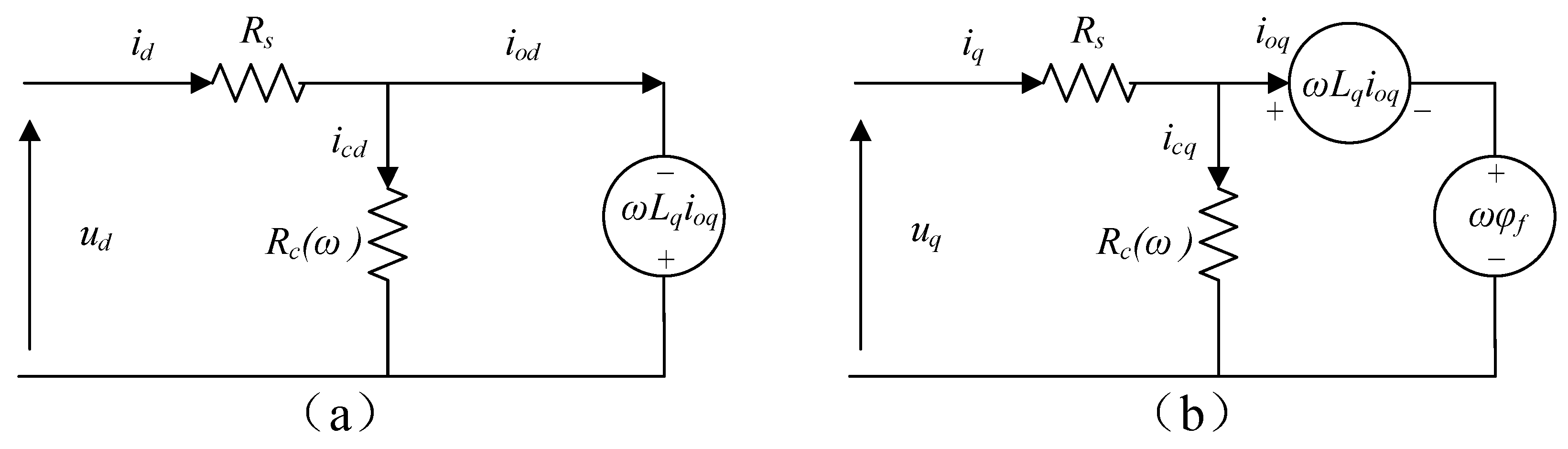
There is always power loss in the working process of a motor, which leads to the fluctuation of speed and torque. The iron loss model can not only reflect the changes of motor voltage, current, flux, and torque, but can also express the changes of the controllable loss including copper loss and iron loss caused by the winding current, which is widely used in the PMSM loss modeling [17]. The equivalent circuit diagram of the PMSM dynamic model employed in this paper is shown in Figure 3. Considering the loss caused by the stator eddy current and hysteresis effect, an iron loss resistance ${\mathrm{R}}_{\mathrm{c}}\left(\mathsf{\omega }\right)$ is added to the equivalent circuit in parallel.

The voltage equivalent equations of the dynamic model are as follows.

$$\left[\begin{array}{c}{\mathrm{u}}_{\mathrm{d}}\\ {\mathrm{u}}_{\mathrm{q}}\end{array}\right]={\mathrm{R}}_{\mathrm{s}}\left[\begin{array}{c}{\mathrm{i}}_{\mathrm{od}}\\ {\mathrm{i}}_{\mathrm{oq}}\end{array}\right]+\left(1+\frac{{\mathrm{R}}_{\mathrm{s}}}{{\mathrm{R}}_{\mathrm{c}}}\right)\left[\begin{array}{c}{\mathrm{u}}_{\mathrm{od}}\\ {\mathrm{u}}_{\mathrm{oq}}\end{array}\right]$$

(1)

$$\left[\begin{array}{c}{\mathrm{u}}_{\mathrm{od}}\\ {\mathrm{u}}_{\mathrm{oq}}\end{array}\right]=\left[\begin{array}{cc}0& -{\mathsf{\omega }\mathsf{\rho }\mathrm{L}}_{\mathrm{q}}\\ {\mathsf{\omega }\mathrm{L}}_{\mathrm{d}}& 0\end{array}\right]\left[\begin{array}{c}{\mathrm{i}}_{\mathrm{od}}\\ {\mathrm{i}}_{\mathrm{oq}}\end{array}\right]+\left[\begin{array}{c}0\\ {\mathsf{\omega }\mathsf{\phi }}_{\mathrm{f}}\end{array}\right]$$

(2)

$$\{\begin{array}{c}{\mathrm{i}}_{\mathrm{od}}={\mathrm{i}}_{\mathrm{d}}-{\mathrm{i}}_{\mathrm{cd}},\\ {\mathrm{i}}_{\mathrm{oq}}={\mathrm{i}}_{\mathrm{q}}-{\mathrm{i}}_{\mathrm{cq}}\end{array}$$

(3)

$$\{\begin{array}{c}{\mathrm{i}}_{\mathrm{cd}}=-\frac{{\mathsf{\omega }\mathsf{\rho }\mathrm{L}}_{\mathrm{d}}{\mathrm{i}}_{\mathrm{oq}}}{{\mathrm{R}}_{\mathrm{c}}},\\ {\mathrm{i}}_{\mathrm{cq}}=\frac{\mathsf{\omega }\left({\mathsf{\phi }}_{\mathrm{f}}+{\mathrm{L}}_{\mathrm{d}}{\mathrm{i}}_{\mathrm{od}}\right)}{{\mathrm{R}}_{\mathrm{c}}}\end{array}$$

(4)

The iron loss resistance ${\mathrm{R}}_{\mathrm{c}}$ is calculated by [18]:

$${\mathrm{R}}_{\mathrm{c}}=\frac{1}{{\mathrm{K}}_{\mathrm{f}}\frac{{\mathrm{K}}_{\mathrm{h}}}{\mathsf{\omega }}}.$$

(5)

Due to the limits of battery voltage, temperature, the bearing capacity of components, and PWM (pulse width modulation) modulation methods, the current and voltage supply capacity of the inverter is limited respectively to ${\mathrm{i}}_{\lim }$ and ${\mathrm{U}}_{\mathrm{dc}\_\lim }$. The motor armature current ${\mathrm{i}}_{\mathrm{s}}$ and terminal voltage ${\mathrm{u}}_{\mathrm{s}}$ expression and constraints are as follows:

$${\mathrm{i}}_{\mathrm{s}}=\sqrt{{\mathrm{i}}_{\mathrm{d}}^2+{\mathrm{i}}_{\mathrm{q}}^2}\le {\mathrm{i}}_{\lim }$$

(6)

$${\mathrm{u}}_{\mathrm{s}}=\sqrt{{\mathrm{u}}_{\mathrm{d}}^2+{\mathrm{u}}_{\mathrm{q}}^2}\le {\mathrm{U}}_{\mathrm{dc}\_\lim }.$$

(7)

The expressions of electromagnetic torque ${\mathrm{T}}_{\mathrm{e}}$ and the motion equation of the PMSM are as follows:

$${\mathrm{T}}_{\mathrm{e}}=\frac{3}{2}{\mathrm{p}}_{\mathrm{n}}\left[{\mathsf{\phi }}_{\mathrm{d}}{\mathrm{i}}_{\mathrm{oq}}+\left({\mathrm{L}}_{\mathrm{d}}-{\mathrm{L}}_{\mathrm{q}}\right){\mathrm{i}}_{\mathrm{od}}{\mathrm{i}}_{\mathrm{oq}}\right]$$

(8)

$${\mathrm{T}}_{\mathrm{e}}={\mathrm{T}}_{\mathrm{L}}+\mathrm{J}\frac{{\mathrm{d}\mathsf{\omega }}_{\mathrm{r}}}{\mathrm{dt}}.$$

(9)

The relationship between ${\mathsf{\omega }}_{\mathrm{r}}\mathrm{and}\mathsf{\omega }$ is as follows:

$${\mathsf{\omega }}_{\mathrm{r}}=\frac{1}{{\mathrm{p}}_{\mathrm{n}}}\mathsf{\omega }=\frac{1}{{\mathrm{p}}_{\mathrm{n}}}\frac{{\mathrm{d}\mathsf{\theta }}_{\mathrm{s}}}{\mathrm{dt}}.$$

(10)

3.2. Speed-Torque-Current Map Integrated Current Control

At present, the control strategies of the motor current mainly include the maximum torque current ratio (MTPA) control, maximum current voltage (MCMV) control, and maximum torque voltage ratio (MTPV) control.

MTPA control is a control method aiming to obtain the maximum output torque with the minimum input of a stator current vector within the limits of voltage and current [19,20]. The control equation of its boundary line is as follows:

$${\mathrm{i}}_{\mathrm{d}}=\frac{-{\mathsf{\phi }}_{\mathrm{f}}+\sqrt{{{\mathsf{\phi }}_{\mathrm{f}}}^2+4{\left({\mathrm{L}}_{\mathrm{d}}-{\mathrm{L}}_{\mathrm{q}}\right)}^2{{\mathrm{i}}_{\mathrm{q}}}^2}}{2({\mathrm{L}}_{\mathrm{d}}-{\mathrm{L}}_{\mathrm{q}})}.$$

(11)

MCMV control is one of the weak magnetic control methods. Its characteristic is that the current vector and voltage vector are the limits of the current and the voltage of the inverter bus, respectively [21]. When the motor speed is adjusted to a certain speed of ${\mathsf{\omega }}_{\mathrm{m}}$, the control equation of (${\mathrm{i}}_{\mathrm{q}}$, ${\mathrm{i}}_{\mathrm{d}}$) in this region is as follows:

$$\{\begin{array}{c}{\mathrm{i}}_{\mathrm{q}}=\frac{\sqrt{{\left(\frac{{\mathrm{U}}_{\mathrm{dc}\_\lim }}{{\mathsf{\omega }}_{\mathrm{m}}}\right)}^2-{\left({\mathrm{L}}_{\mathrm{d}}{\mathrm{i}}_{\mathrm{d}}+{\mathsf{\phi }}_{\mathrm{f}}\right)}^2}}{{\mathrm{L}}_{\mathrm{q}}}\\ {\mathrm{i}}_{\mathrm{d}}=-\sqrt{{\mathrm{i}}_{\lim }^2-{\mathrm{i}}_{\mathrm{q}}^2} \end{array}.$$

(12)

MTPV control enables the motor to achieve the maximum speed by making full use of the voltage vector supplied by the inverter [22,23,24]. For the tab-mounted PMSM, the reference current vector and the voltage control equation of MTPV is as follows:

$$\{\begin{array}{c}{\mathrm{i}}_{\mathrm{d}}=\frac{-{\mathsf{\phi }}_{\mathrm{f}}}{{\mathrm{L}}_{\mathrm{d}}} \\ {\mathrm{i}}_{\mathrm{q}}=-\frac{{\mathrm{U}}_{\mathrm{dc}\_\lim }}{{\mathrm{L}}_{\mathrm{q}}{\mathsf{\omega }}_{\mathrm{s}}}\end{array}$$

(13)

$$\{\begin{array}{c}{\mathrm{u}}_{\mathrm{q}}=\frac{{\mathsf{\phi }}_{\mathrm{f}}-\sqrt{{{\mathsf{\phi }}_{\mathrm{f}}}^2+8{\mathrm{U}}_{\mathrm{dc}\_\lim }^2{\left(\frac{{\mathrm{L}}_{\mathrm{d}}-{\mathrm{L}}_{\mathrm{q}}}{{\mathrm{L}}_{\mathrm{q}}{\mathsf{\omega }}_{\mathrm{s}}}\right)}^2}}{-4\left(\frac{{\mathrm{L}}_{\mathrm{d}}-{\mathrm{L}}_{\mathrm{q}}}{{\mathrm{L}}_{\mathrm{q}}{\mathsf{\omega }}_{\mathrm{s}}}\right)}\\ {\mathrm{u}}_{\mathrm{d}}=-\sqrt{{\mathrm{U}}_{\mathrm{dc}\_\lim }^2-{\mathrm{u}}_{\mathrm{q}}^2} \end{array}.$$

(14)

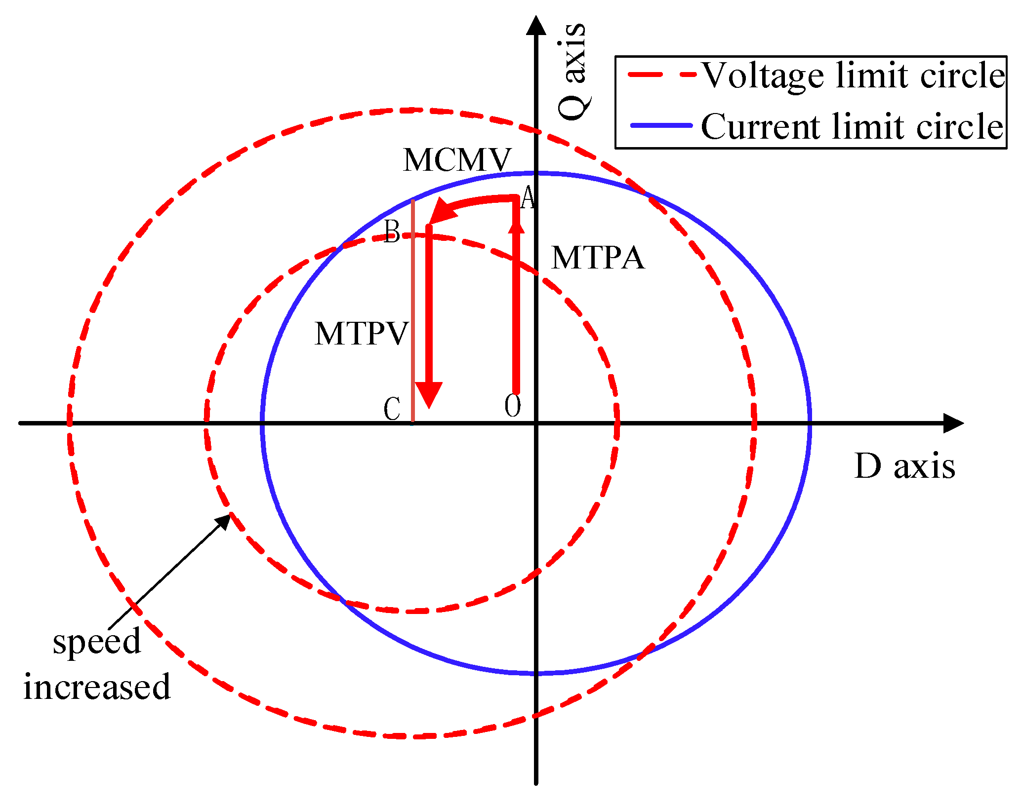
To sum up, the running trajectories of the boundaries of the three control strategies in the d-q coordinate system are shown in Figure 4. OA, AB, and BC represent the running trajectories of the three control strategies (MTPA, MCMV, and MTPV) in the d-q coordinate system, respectively.

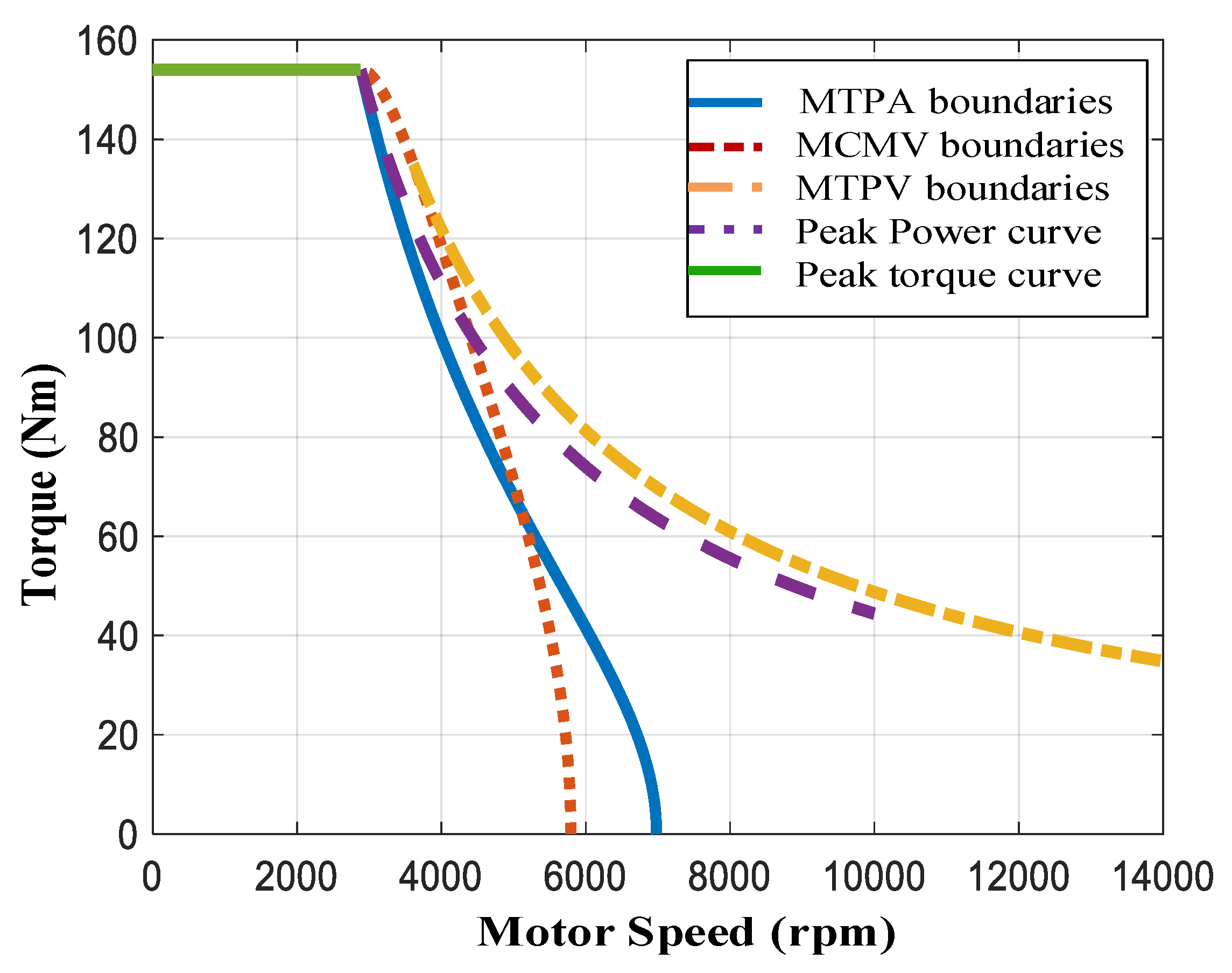
To analyze the influence of different current control strategies on the motor speed–torque characteristics, the external characteristics under different strategies are obtained, as shown in Figure 5.

Aiming to combine the advantages of the above three control strategies, a comprehensive control strategy is proposed in this paper to expand the motor working range to its maximum within the scope of the inverter bus capacity. The principles of the comprehensive control strategy are as follows:

(a)

The MTPA control strategy is adopted in the peak torque area to minimize the copper loss and iron loss.

(b)

In the high-torque region of the weak magnetic field, the MCMV control is adopted to transit to the MTPV control range.

(c)

MTPV control is used to extend the speed range of the motor in the high-speed region of the weak magnetic field.

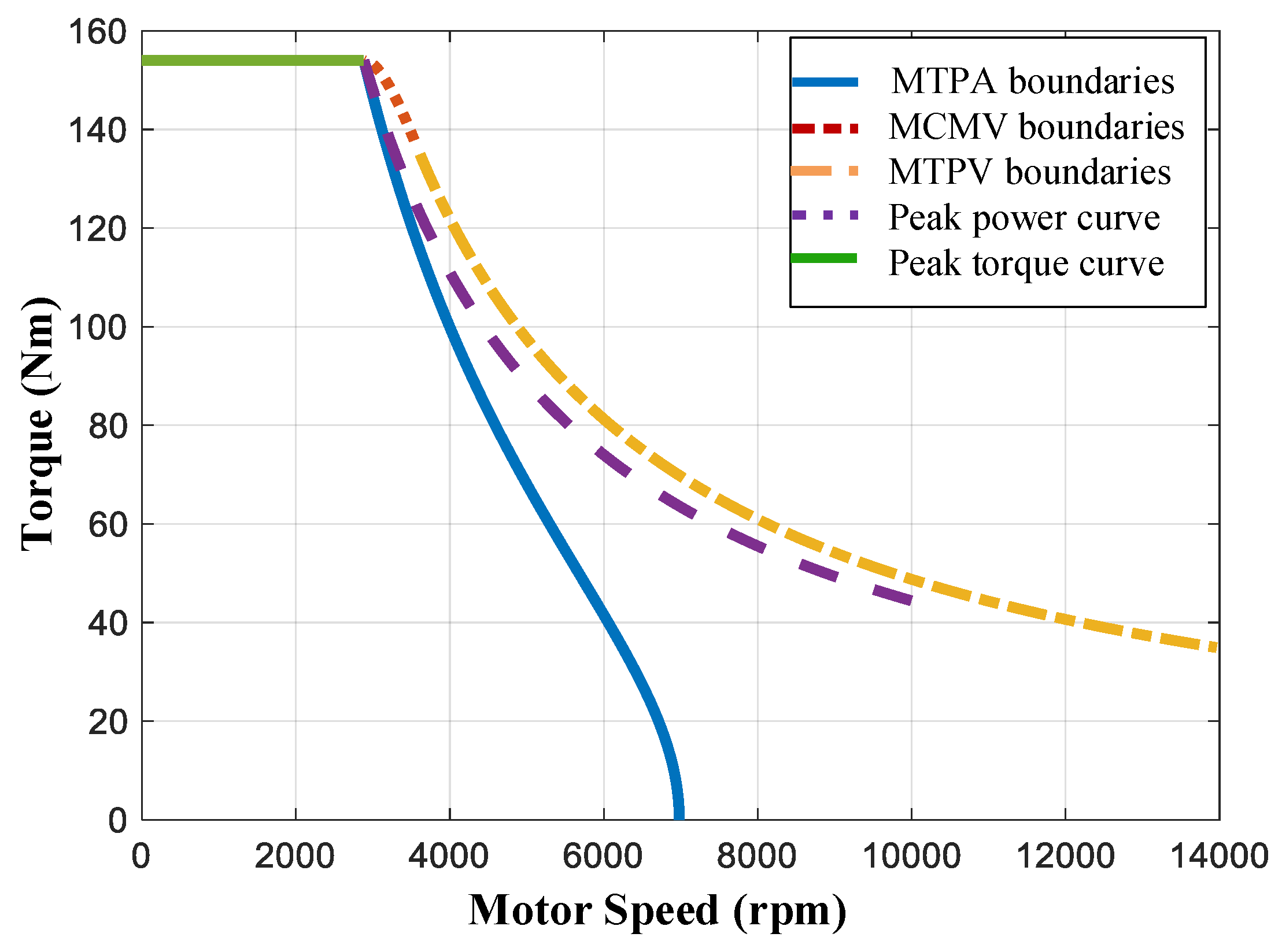
With the above principles, the external characteristic boundary of current control is obtained, as shown in Figure 6. Compared with the single current control strategy, the designed comprehensive control strategy has a wider speed range under the same torque, which improves the utilization ratio of the input current vector and voltage vector and maximizes the overall working range of the motor.

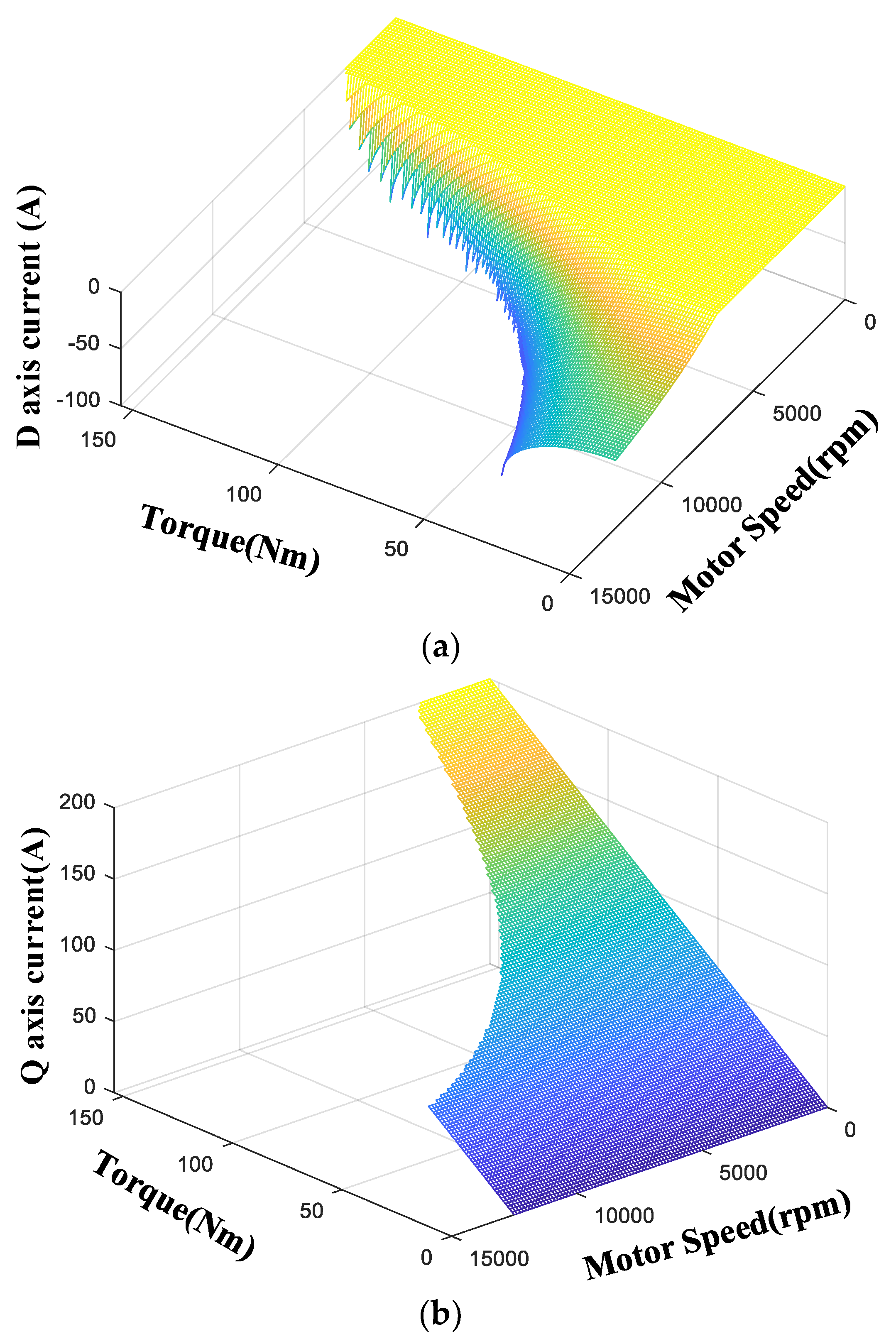
Based on the designed current control boundary curve, the speed and torque are traversed and substituted into Equations (8) and (9) to obtain the current of the d axis and q axis of all the work points. The resulting speed–torque–current map of the d-axis and q-axis are shown in Figure 7.

3.3. Motor Vector Control Strategy

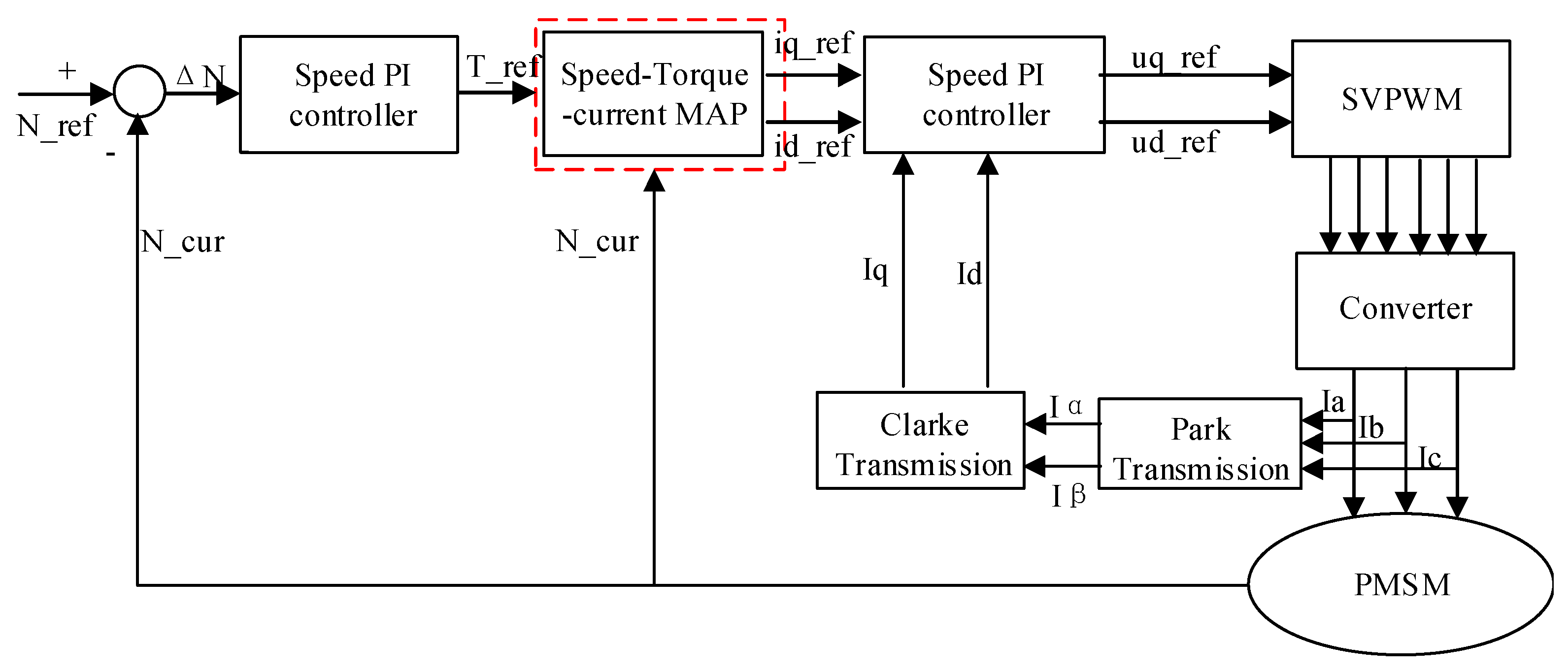
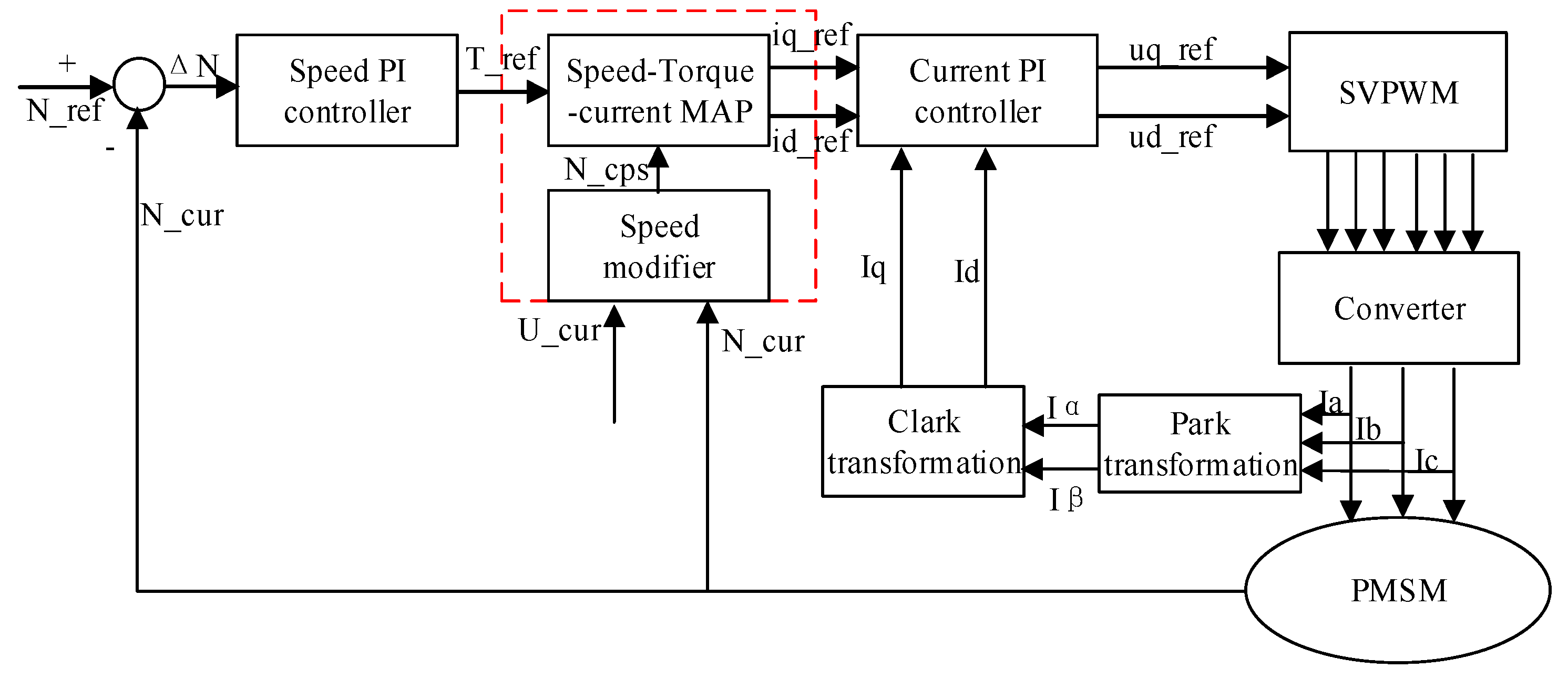
In order to solve the nonlinear problem of the PMSM current in the weak magnetic region, a vector control strategy is designed for the motor based on the speed–torque–current map, as shown in Figure 8. When the motor runs in the weak magnetic region, the d and q-axis currents are obtained using the lookup table method. This method avoids the control problems caused by the nonlinear current, which in turn extends the weak magnetic working region of the motor. It is convenient to obtain the current in the deep weak magnetic region by using the lookup table. Besides, the following problems can also be solved: it is difficult to obtain the current simply by using the weak magnetic PI controller, and the dynamic response of the motor is slow.

As shown in Figure 8, a speed–torque–current map link is added to the vector control strategy between the speed control link and the current control link. The output reference torque ${\mathrm{T}}_{\_\mathrm{ref}}$ of the speed loop and the actual motor speed are the inputs to this link. The reference currents of the d and q axes corresponding to the current speed and the target torque can be obtained by a lookup table. Since the speed–torque–current map contains the information of the weak magnetic region (including the deep weak magnetic region), the currents of the d and q axes are constrained in the voltage limit circle and current limit circle. It solves the transition problems of current control in different working ranges and the problem of torque fluctuation caused by current or voltage over-saturation.

Charging and discharging are always present in the driving process of pure electric vehicles, which leads to the change of battery SOC (state of charge). The relationship between the battery voltage and SOC is shown in Figure 9. The change of the battery voltage causes the dynamic change of bus voltage amplitude [25], which in turn affects the d-axis current and q-axis current, as well as the speed and torque characteristics of the motor.

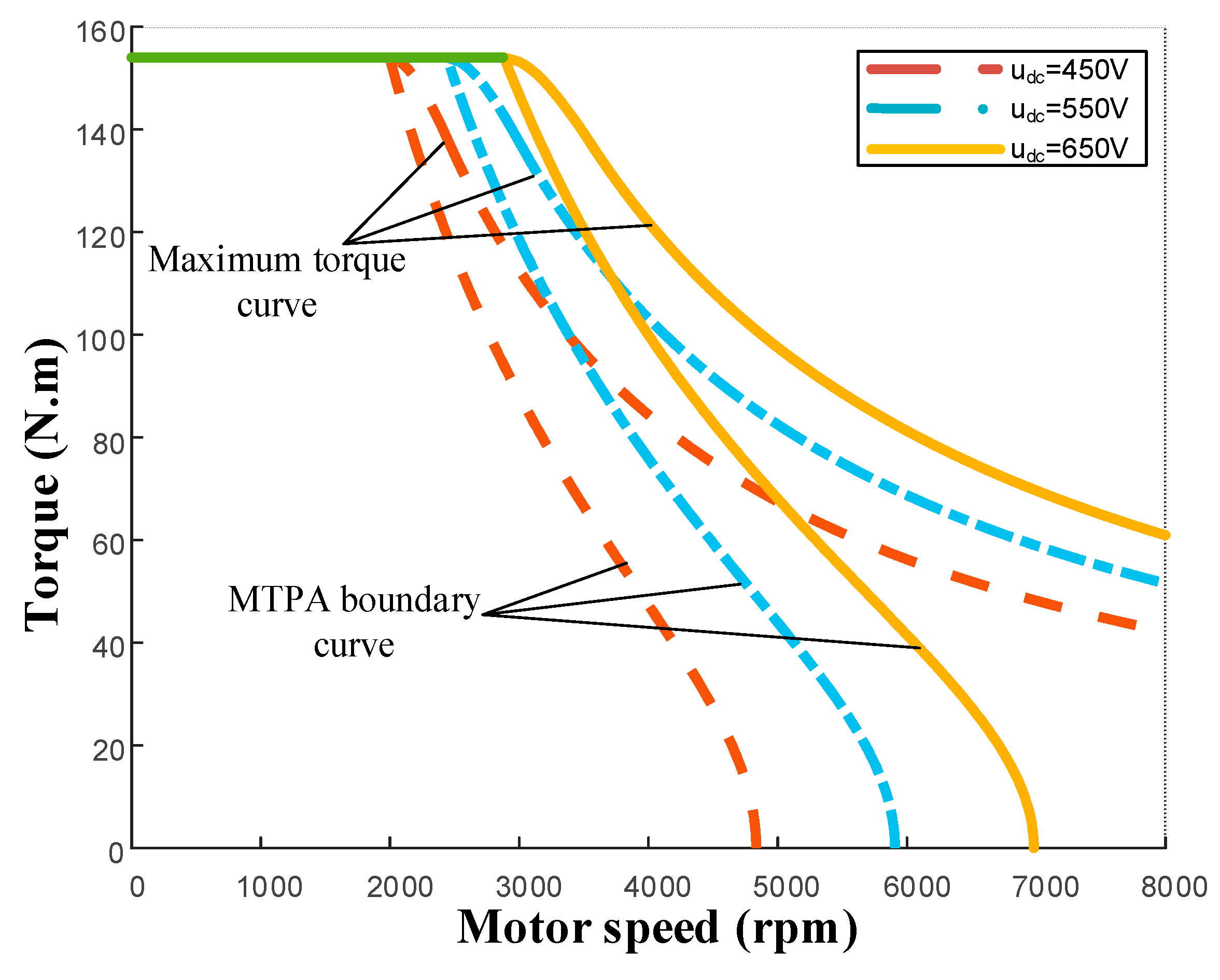
The external characteristics of the motor under different bus voltages are shown in Figure 10.

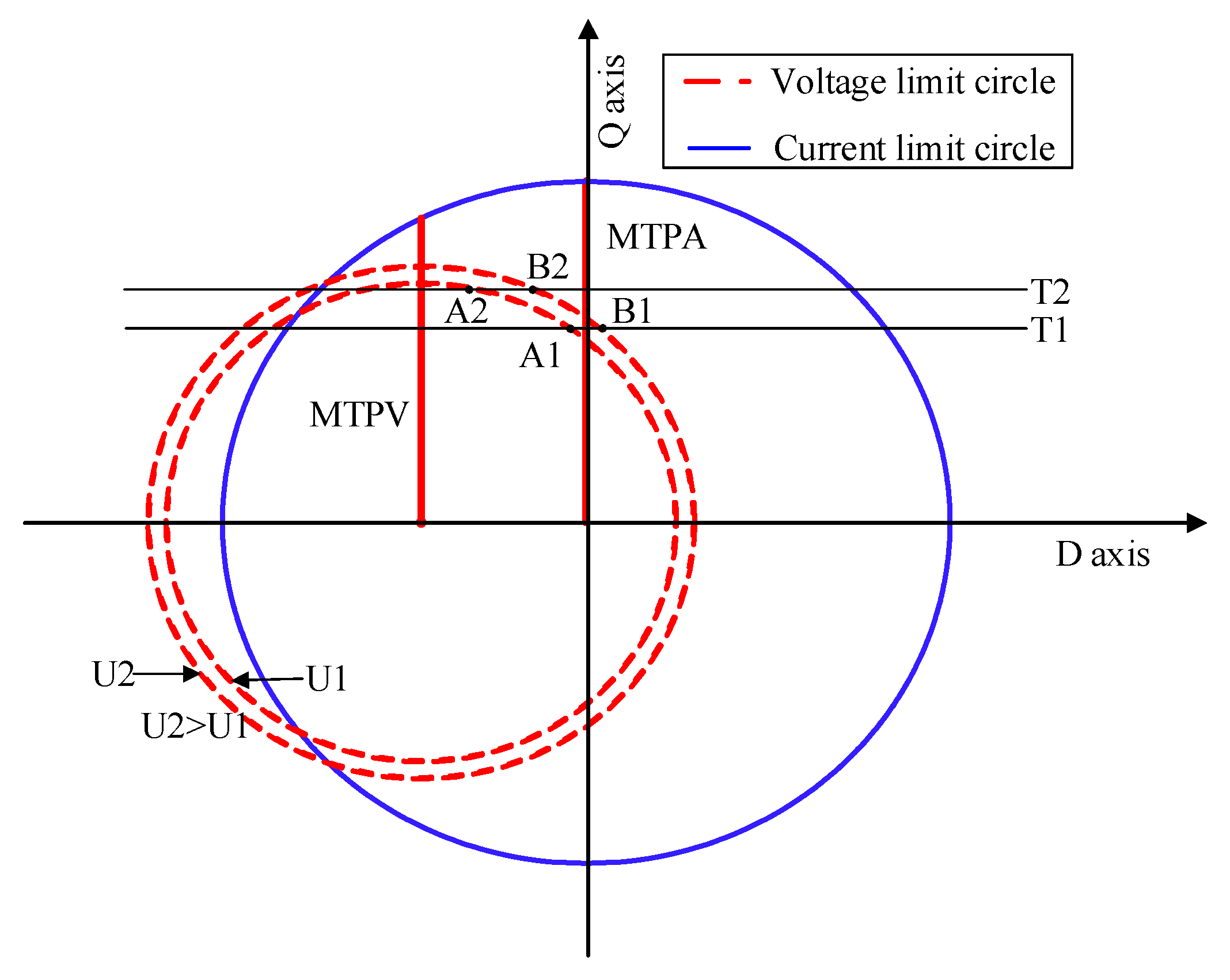
It is shown in Figure 10 that when the bus voltage decreases, the control boundary and the maximum torque boundary of the motor move to the left, which reduces the motor working range. If the influence of bus voltage variation is ignored, the operation of these areas cannot be controlled. When the voltage increases, the bus voltage cannot be fully utilized. When the voltage decreases, the working point may be outside the allowable motor working range, which leads to the over-current or over-voltage protection. The influence of bus current on the motor can also be seen from the perspective of current control of d and q axes, which is shown in Figure 11. When the bus voltage is $\mathrm{U}1$, the motor works at points $\mathrm{A}1$ and $\mathrm{A}2$ to realize torques $\mathrm{T}1$ and $\mathrm{T}2$, respectively. If the bus voltage increases from $\mathrm{U}1$ to $\mathrm{U}2$, then the motor working points are $\mathrm{B}1$ and $\mathrm{B}2$, which improves the utilization ratio of the bus voltage. On the contrary, if $\mathrm{T}1$ and $\mathrm{T}2$ are the required torques, the motor works at points $\mathrm{B}1$ and $\mathrm{B}2$. If the bus voltage decreases from $\mathrm{U}2$ to $\mathrm{U}1$ and the control strategy still takes $\mathrm{B}1$ and $\mathrm{B}2$ as working points. In this situation, the current regulator saturates and loses its ability to regulate the current.

Considering the fluctuation of bus voltage, the relationship between the actual bus voltage ${\mathrm{U}}_{\mathrm{dc}\_\mathrm{act}}$ and the currents of the d and q axes is as follows:

$${\left(\frac{{\mathrm{U}}_{\mathrm{dc}\_\mathrm{act}}}{{\mathsf{\omega }}_{\mathrm{s}}}\right)}^2={({\mathrm{L}}_{\mathrm{q}}{\mathrm{i}}_{\mathrm{q}})}^2+{({\mathrm{L}}_{\mathrm{d}}{\mathrm{i}}_{\mathrm{d}}+{\mathsf{\phi }}_{\mathrm{f}})}^2.$$

(15)

Equation (15) indicates that the bus voltage fluctuation can be corrected by the motor speed. Specifically, when the bus voltage changes, the motor speed can be appropriately increased or decreased by $\mathsf{\mu }$ times to correct the voltage, as shown in the following equation:

$$\{\begin{array}{c}\mathsf{\mu }=\frac{{\mathrm{U}}_{\mathrm{dc}\_\lim }}{{\mathrm{U}}_{\mathrm{dc}\_\mathrm{act}}} \\ {\left(\frac{{\mathrm{U}}_{\mathrm{dc}\_\lim }}{{\mathsf{\omega }}_{\mathrm{s}}\mathsf{\mu }}\right)}^2={({\mathrm{L}}_{\mathrm{q}}{\mathrm{i}}_{\mathrm{q}})}^2+{({\mathrm{L}}_{\mathrm{d}}{\mathrm{i}}_{\mathrm{d}}+{\mathsf{\phi }}_{\mathrm{f}})}^2\end{array}.$$

(16)

Based on Equation (16), a speed modifier considering the influence of bus voltage is added to the speed–torque–current map link to develop a vector control strategy, as shown in Figure 12. The real-time bus voltage ${\mathrm{U}}_{\_\mathrm{cur}}$ obtained from the voltage sensor is used as the input to the speed compensator, and variable ${\mathrm{N}}_{\_\mathrm{cps}}$ represents the speed after the compensation.

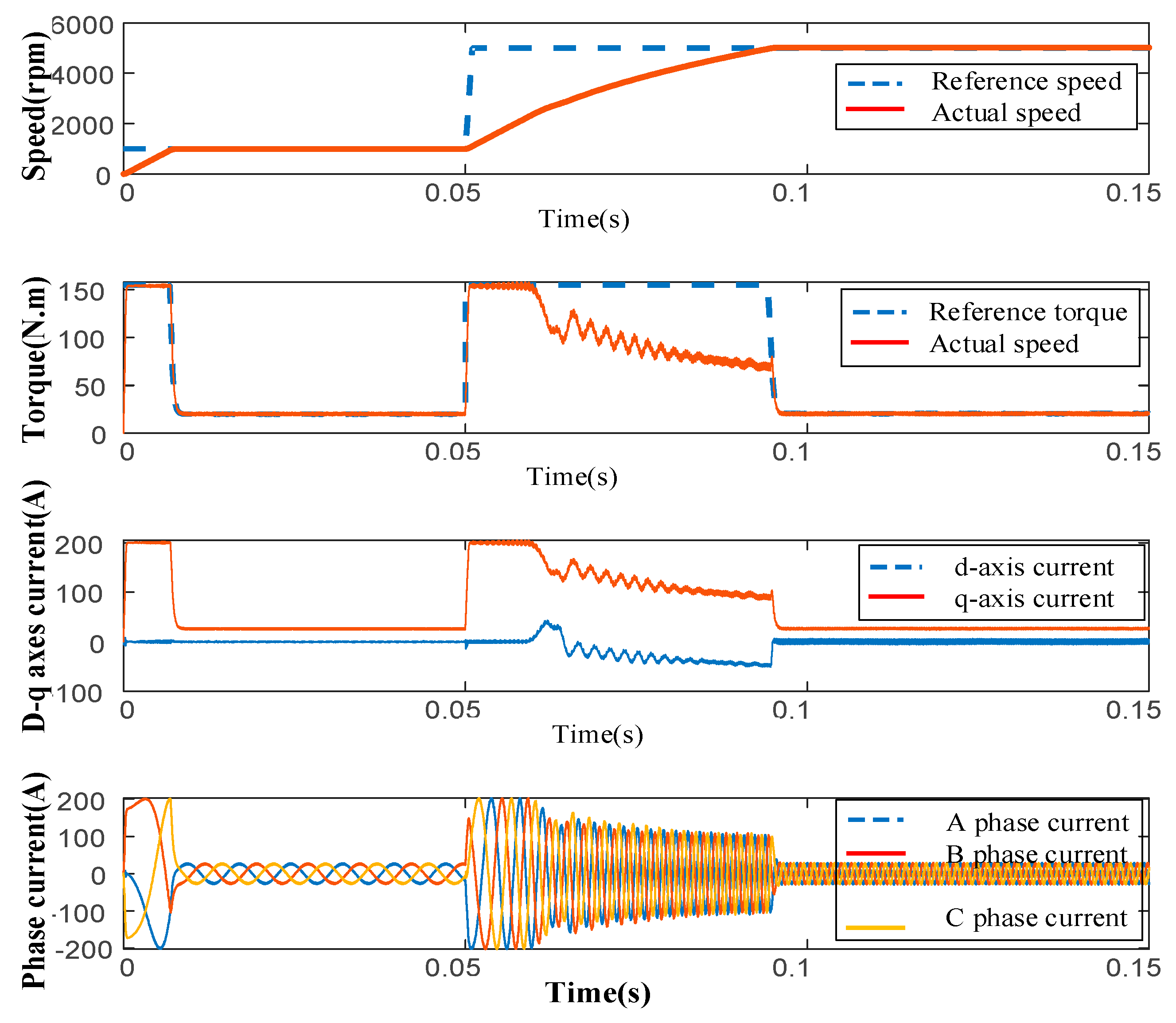
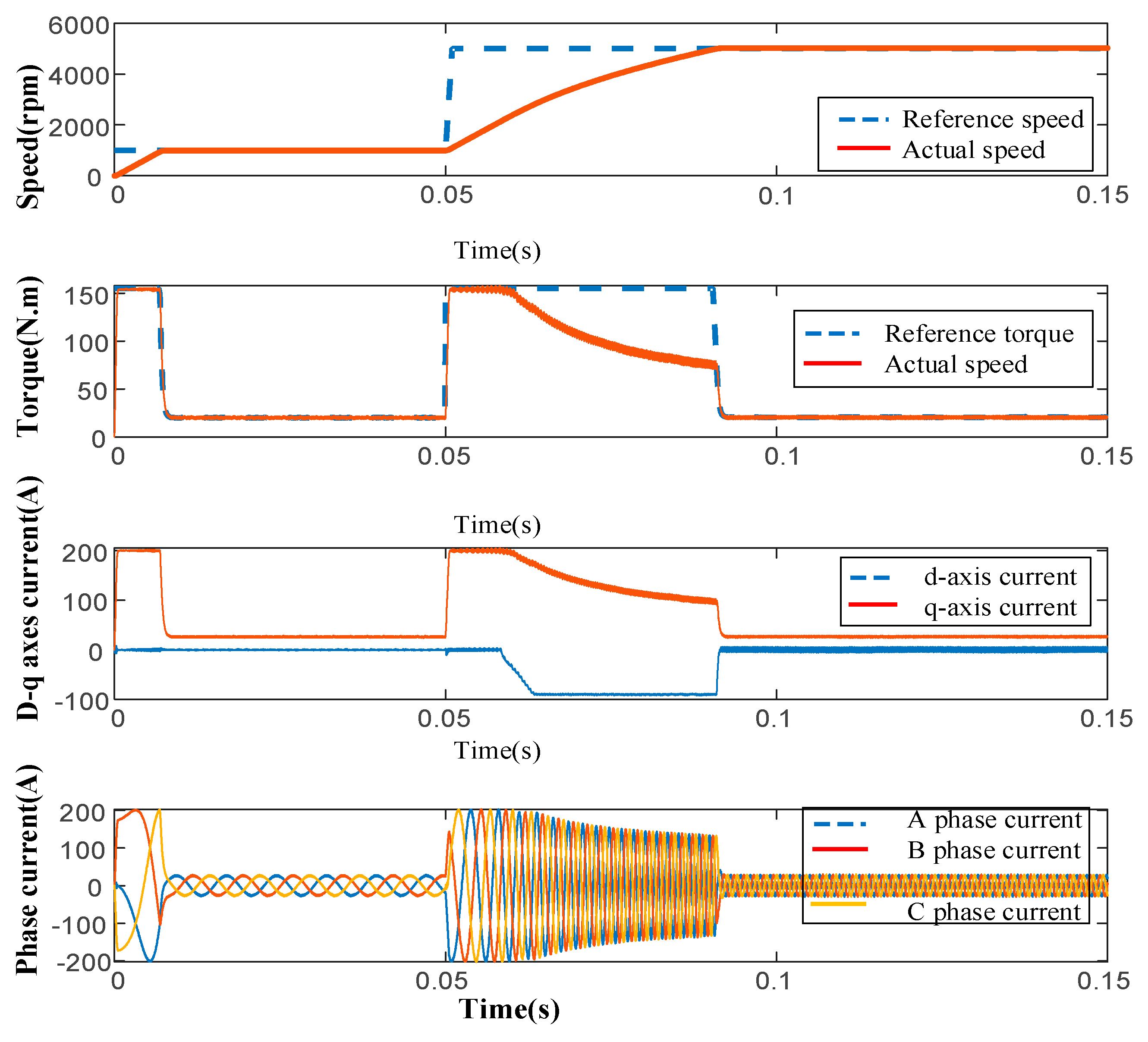
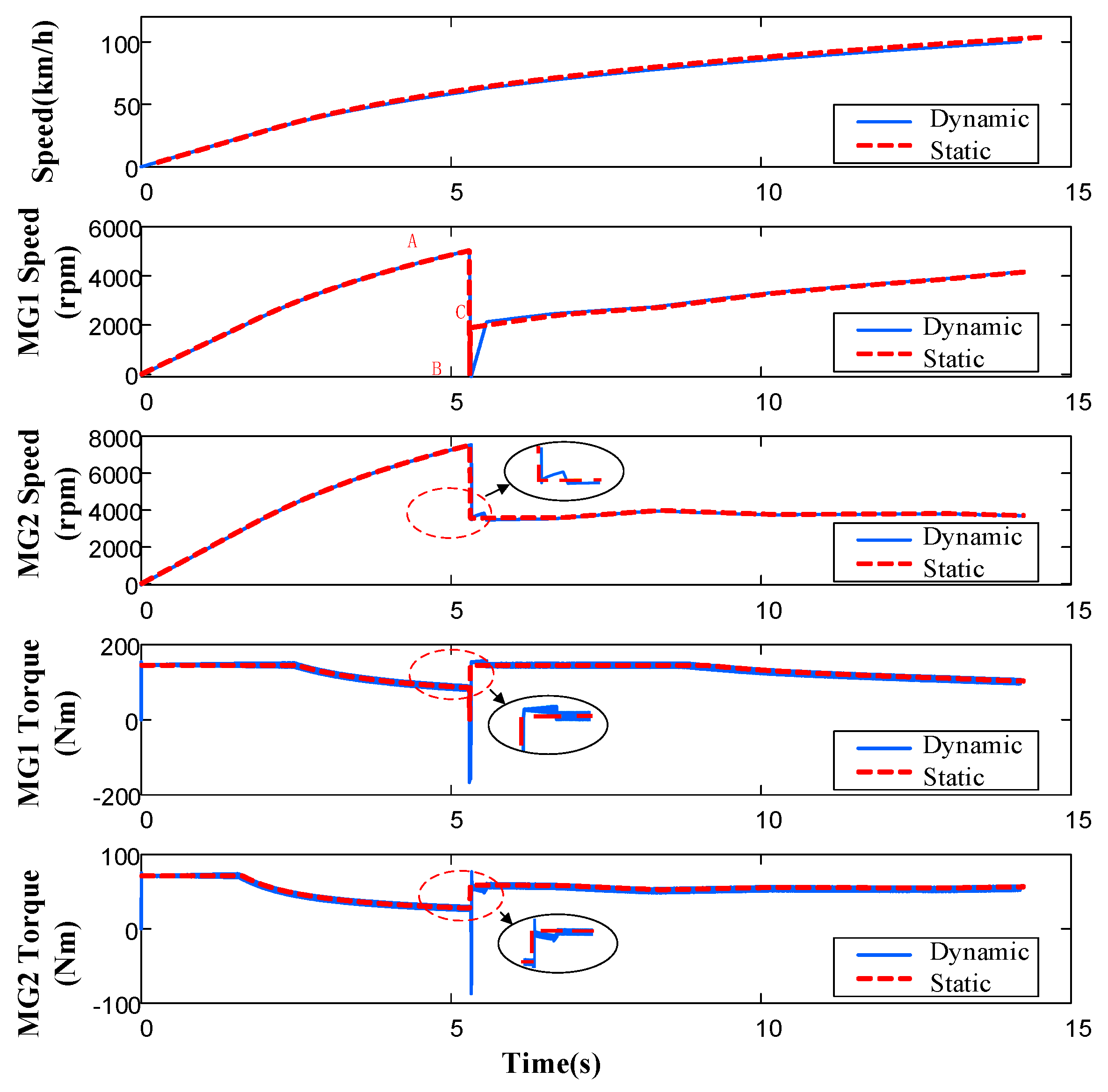
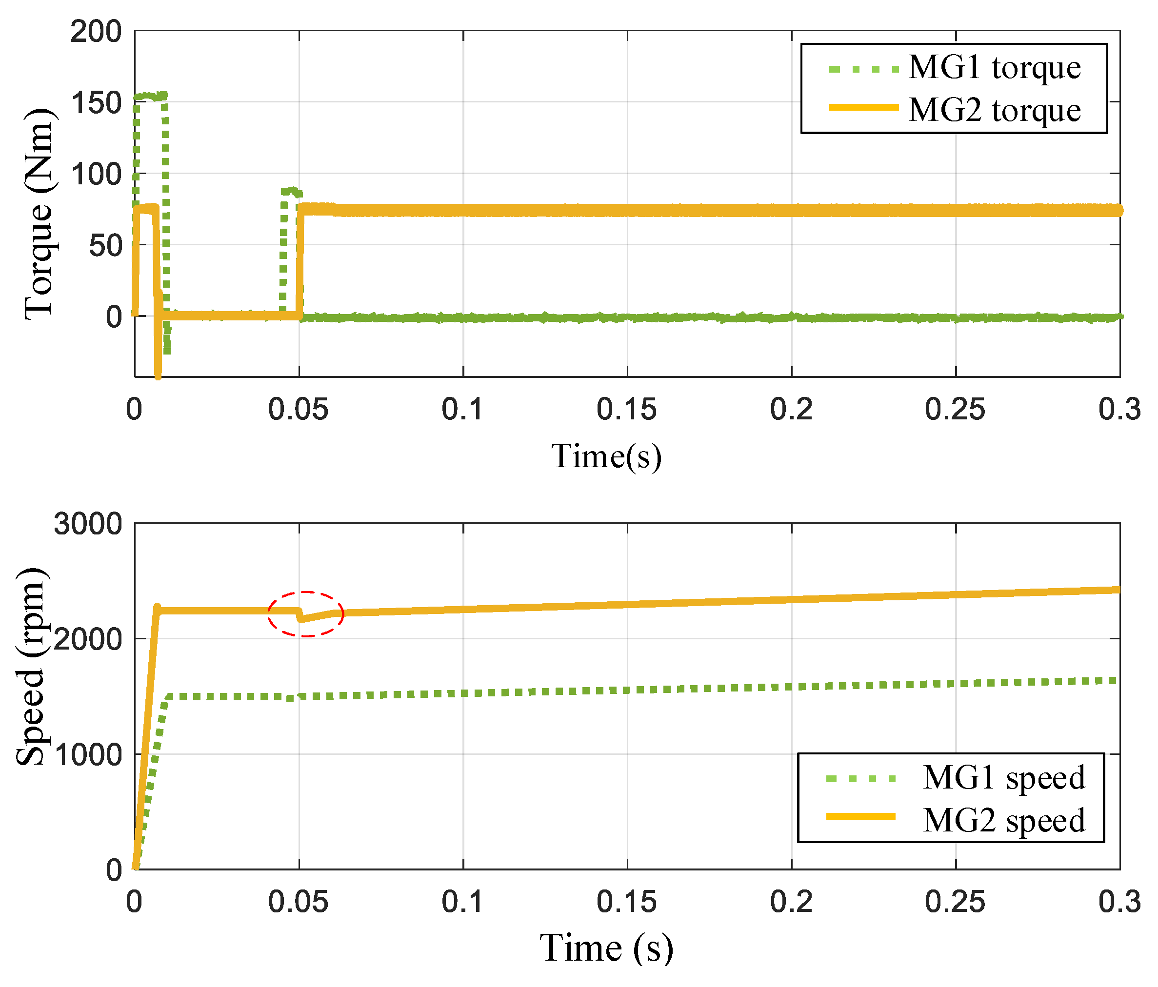
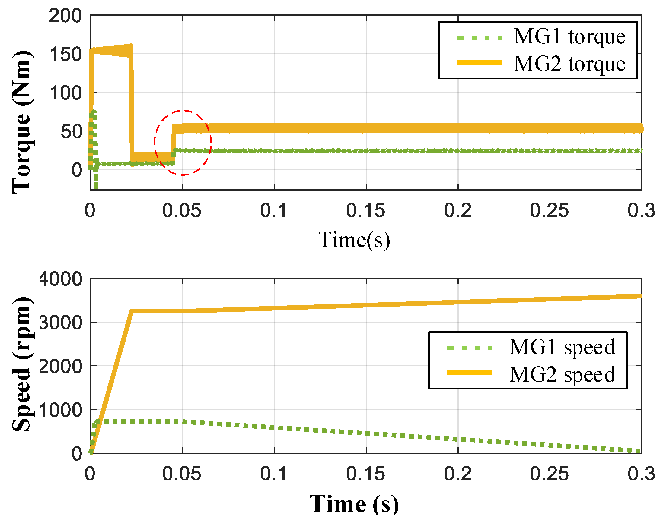
To validate the control effect of the proposed vector control strategy, a working condition is designed in which the bus voltage and load torque are 650 V and 20 Nm, respectively. Besides, the motor speed first accelerates from 0 to 1000 rpm, and then again accelerates from 1000 to 5000 rpm after the speed stabilizes for a short period (around 100 ms). The simulation results are shown in Figure 13 and Figure 14.

It is seen from Figure 13 that in the process of speed regulation, torque and current fluctuate greatly due to the effect of the bus voltage changes. However, in Figure 14, the current and torque fluctuations are greatly reduced during the speed regulation period (1000–5000 rpm), when the bus voltage changes are taken into consideration. The results in these two figures indicate that the speed modifier with bus voltage regulation well reduces the torque and current fluctuation in the speed regulation process, which is beneficial to the output speed–torque characteristics of the motor.

4. Verification of the Proposed Vector Control Strategy

4.1. System Power Distribution Strategy

In the actual operation process of the motor, when the output demand is constant, the position of the working point has an impact on the speed regulation process and the energy consumption of the motor. However in the static model, the working point is well determined. Based on vehicle model and PMSM dynamic model established in the previous section, the speed–torque characteristics and the energy consumption characteristics of system are analyzed when the system demand changes. In the coupling modes, the torque distribution strategy and speed distribution strategy are shown in Figure 15 and Figure 16, respectively.

Due to the difference between the static model and the actual operation, the minimum energy consumption point calculated by the static model may not be accurate for the motor. Therefore, the power distribution strategy based on the dynamic control enables the vehicle to operate at the working point with the minimum energy demand, thereby reducing the vehicle energy consumption.

4.2. Simulation Analyses

Based on the configuration considered in this paper, two vehicle models which are configured with the static and dynamic models are established for simulation studies. The following three working conditions are employed for verification purposes: 0–100 km acceleration, torque coupling mode, and speed coupling mode.

4.2.1. 0–100 km/h Acceleration Simulation

In the simulation of 0–100 km/h acceleration, when the vehicle speed is lower than 60 km/h, the torque coupling mode is adopted; otherwise, the speed coupling mode is adopted. The results are shown in Figure 17.

Response delay and torque fluctuation always exist in the actual process of motor speed regulation. Figure 17 shows that due to the response delay, the 0–100 km/h acceleration time resulting from the dynamic model is 14.22 s, which is 0.12 s more than that of the static model (14.10 s). The reason is that the speed and torque response characteristics of the dynamic model are closer to the actual motor operating characteristics. Different from the step response in the mode switching process of the static model, it can be seen from the speed diagram that the time required for the motor to complete mode switching is almost 0.28 s in the dynamic model, which is not shown in the static model. Torque fluctuation always exists in the dynamic model but not in the static model. The fluctuation in the process of mode switching is more apparent, which is shown in the enlarged red circle areas for the torques of MG1 and MG2. In this process, the torque of MG1 is greater than that of the static model, and the torque of MG2 is less than that of the static model. The lines of the torque aligned with the static model after 5.57 s because in the mode switching process, the speed regulation of the two motors caused the change of motor torque. This situation is similar to the actual motor operation, indicating that the dynamic model can well reflect the actual motor speed regulation process.

4.2.2. Torque Coupling Mode Performance Simulation

According to the flow shown in Figure 15, the designed simulation condition of the torque coupling mode is as follows: during the period from 0 to 0.05 s, the vehicle speed is adjusted to 18 km/h. In this process, the torque is adjusted to the required torque. After 0.05 s, the vehicle accelerates to 19.7 km/h with 1.8889 m/s² acceleration during 0.25 s. When the vehicle speed is 18 km/h and the acceleration is 1.8891 m/s², the required torque and speed of the main reducer are 224 Nm and 720 rpm, respectively. According to the dynamic equation of the torque couple mode, the speeds of MG1 and MG2 are 1494 rpm and 2237 rpm, respectively. Under the corresponding speed constraint, the maximum electromagnetic torques of MG1 and MG2 can achieve 153 Nm and 75 Nm, respectively. The torque intervals of MG1 and MG2 are [−153 Nm, 153 Nm] and [−75 Nm, 75 Nm], respectively. Moreover, the torques of MG1 and MG2 (i.e., ${\mathrm{T}}_{\mathrm{m}1}$ and ${\mathrm{T}}_{\mathrm{m}2}$) are also limited by the demand torque ${\mathrm{T}}_{\mathrm{o}}$ of the main reducer, namely:

$${\mathrm{T}}_{\mathrm{o}}={\mathrm{T}}_{\mathrm{m}2}·\left(\mathrm{k}+1\right)·{\mathrm{i}}_2·{\mathsf{\eta }}_2·{\mathsf{\eta }}_{\mathrm{p}}+{\mathrm{T}}_{\mathrm{m}1}·{\mathrm{i}}_1·{\mathsf{\eta }}_1.$$

(17)

The motor electromagnetic torque is the sum of the load torque and the speed regulating torque. If the load torque is too large, the motor will lose the ability to regulate the speed. In order to meet the requirements of the output characteristics of the main reducer, the initial and target torques of MG1 are limited in the range of [−2 Nm, 148 Nm] based on Equation (17).

Under the same working condition, the torque of MG1 is 88 Nm according to the motor static model control strategy, which is set as the initial MG1 torque. That is, T1 = 88 Nm. In this section, the MG1 target load torque value (T1* = −2 Nm) is taken as an example to analyze the speed–torque characteristics during the transition process of two motor working points under this working condition. The dynamic response process of the two motors is shown in Figure 18.

Figure 18 demonstrates the change of the two motor speeds, as the vehicle speed is adjusted to 18 km/hat, no load condition during the period of 0–0.045 s. In the period of 0.045–0.05 s, the torques of the two motors are adjusted to the demand torque corresponding to the condition (i.e., 18 km/h vehicle speed and 1.8991 m/s2 acceleration. At the moment of 0.05 s, the motor MG1 is loaded by the target torque of −2 Nm, and the torque of MG2 is calculated from the real-time load torque and the load torque of MG1.

In the torque coupling mode, the torques of MG1 and MG2 can be coupled arbitrarily, as long as the output torque of the vehicle meets requirements. This means that countless combinations of the torques of MG1 and MG2 exist. The economy of each combination can be measured by the demand power of the electric drive system. According to the flow shown in Figure 16, the MG1 target torque is traversed to obtain the corresponding demand power of the electric drive, as shown in Figure 19.

When the demand torque is constant in the torque coupling mode, the torque of MG1 is 88 Nm on the point of the allocated power obtained from the static model. In the dynamic model, the demand power of the electric drive system first decreases and then increases with the increase of the MG1 target torque, as shown in Figure 19. Note that the starting point ${T_1}^{*}$ = −2 Nm, the final point ${T_1}^{*}=148\mathrm{Nm}$, and the trough point ${T_1}^{*}=68\mathrm{Nm}$ are employed in the simulation studies, as shown in

Table 4. Demand power under different MG1 target torques.

MG1 Target Torque/Nm	MG1 Power/kW	MG2 Power/kW	Demand Power/kW
−2	0.248	25.856	26.104
68	13.476	8.073	21.549
88	17.814	4.007	21.822
148	32.297	−5.157	27.140

.

The motor static model cannot reflect the loss during the transition process of the motor working point, so the optimal power distribution scheme of the two motors cannot be obtained when the power demand of the system is fixed. If the vehicle demand torque is constant, MG1’s target torque is too high, which results in MG1 working near the peak torque. If the target torque of MG1 is too small, then MG2 will work near its peak torque, and vice versa. These situations will lead to an increase in system losses and lower efficiency. The transformation law of demand power with MG1 target torque is shown in Figure 19, when the demand torque is constant. Table 4 shows that when the MG1 target torque is 148 Nm, the demand power of the electric power system reaches a maximum of 27.140 kW. When the target torque is 88 Nm in the static model, the average demand power of the system is 21.822 kW. When the target torque is 68 Nm (obtained from the dynamic model), the demand power of the system has a minimum of 21.549 kW, which is 1.27% lower than the average power consumption obtained by the static model, and 20.6% lower than the maximum demand power of the electric drive system.

4.2.3. Speed Coupling Mode Performance Simulation

In the speed coupling mode, when the required torque is constant, the speeds of both motors can change within a certain range, and the system power consumption corresponding to different speed combinations is also different. According to the flow shown in Figure 16, the simulation condition is designed as follows: from 0 to 0.05 s, the vehicle speed is adjusted to 60 km/h. In this process, the torque is adjusted to the demand torque. Then, the vehicle travels from the initial speed of 60 km/h to the target speed of 60.43 km/h, with an acceleration of 0.48 m/s² for 0.25 s.

Under the above conditions, the demand torque and speed of the main reducer are 75 Nm and 2430 rpm, respectively. The corresponding torques of MG1 and MG2 are 51 Nm and 24 Nm, respectively. Under the restriction of corresponding speed, the maximum speeds of MG1 and MG2 are 5600 rpm and 8500 rpm, respectively. The speed ranges of MG1 and MG2 are [−5600 rpm, 5600 rpm] and [−8500 rpm, 8500 rpm], respectively. In addition, the speeds of MG1 and MG2 are also constrained by the demand speed of final drive, which is described as follows:

$${\mathsf{\omega }}_{\mathrm{o}}=\frac{{\mathsf{\omega }}_{\mathrm{m}1}·\mathrm{k}+{\mathsf{\omega }}_{\mathrm{m}2}}{{\mathrm{i}}_0·\left(\mathrm{k}+1\right)}.$$

(18)

To meet the requirements of the main reducer output characteristics, the speed range of MG1 under this condition is [−295 rpm, 5600 rpm] based on Equation (18).

The target speed ${{\mathrm{n}}_1}^{*}=3590\mathrm{rpm}$ of MG1 is taken as an example to analyze the speed–torque characteristics during the working point transfer process. The dynamic responses of MG1 and MG2 are shown in Figure 20.

As shown in Figure 20, in the period of 0–0.045 s, the speed of the two motors are adjusted to the speed when the vehicle speed is 60 km/h. In the period of 0.045–0.05 s, the torques of the two motors are adjusted to the demand torque corresponding to the condition (i.e., 60 km/h speed and 0.48 m/s² acceleration). At the moment of 0.05 s, the MG1 speed is adjusted to the target speed of 3590 rpm; meanwhile, the torque of MG1 increases and that of MG2 decreases as these two motors need extra torque to overcome the rotational inertia force when the speed changes.

According to the power distribution flow in Figure 16, all of the energy consumption corresponding to the target speed n1* of MG1 can be obtained. When the vehicle speed is 60.43 km/h, the range of n1* is [−295 rpm, 5600 rpm]. When the initial speed of MG1 is set to 3242 rpm, the target speed of MG1 traverses in the interval of [−295 rpm, 5600 rpm] to obtain the demand power of the electric drive system. The demand power of the system, corresponding to different target speeds of MG1, is shown in Figure 21.

The optimal speed of MG1 $\mathrm{n}1$* obtained from the static model of the motor is 3590 rpm. In the dynamic model, it is seen from Figure 21 that with the increase of target speed n1* of MG1, the system demand power first decreases and then increases. The following points of the MG1 target speed n1* are selected in the simulation studies: the starting point of the decreasing function is −295 rpm, the trough point is 1867 rpm, and the final point of the increasing function is 5600 rpm.

Table 5. Demand power of the electric drive system at different MG1 target speeds.

MG1 Target Speed/rpm	MG1 Power/kW	MG2 Power/kW	Demand Power/kW
−295	7.615	16.291	23.906
1867	14.347	7.745	22.092
3590	21.53	2.013	23.543
5600	31.56	−2.965	28.595

shows the demand power at different MG1 target speeds.

Table 5 shows that the power of MG1 increases and that of MG2 decreases, with the increase of the MG1 target speed n1*. When the optimal speed (3590 rpm) obtained by the static model is taken as the target speed of MG1, the average demand power of the drive system is 23.543 kW, which is not the minimum demand power of the electric drive system under this condition. When the MG1 target speed n1* is 5600 rpm, the maximum power demand of the electric drive system is 28.595 kW. This is because when the target speed of MG1 is 5600 rpm, the speeds of motor MG1 and MG2 need to be adjusted from 3242 rpm to 5600 rpm, and from 733 rpm to −4165 rpm, respectively. This is a large speed regulation process, which leads to power loss. When the target speed of MG1 is 1867 rpm, the minimum demand power of the electric drive system can be obtained, i.e., 22.092 kW. This minimum value is 6.16% lower than the average demand power obtained from the static model and 22.74% lower than the maximum demand power of the electric drive system.

5. Conclusions

In this paper, the mechanical and electrical energy conversion mechanism and dynamic control of PMSM are studied in order to analyze the impact on the performance of pure electric vehicle. Considering the influence of bus voltage fluctuation on motor performance, a vector control strategy based on the speed–torque–current map is designed. In this study, three working conditions were formulated, including the 0–100 km/h acceleration condition, speed coupling condition, and torque coupling condition. They have been used to study the dynamic characteristics and energy consumption characteristics of the double motor coupling mode. The simulation results show that compared to the static control model, the dynamic control model can better reflect the actual working process of the motor. In the torque coupling mode, the minimum demand power of the system, corresponding to the optimal MG1 target torque, is obtained from the dynamic characteristics of the motor. This power is 1.27% lower than that obtained from the static model and 20.6% lower than the maximum demand power of the system. In the speed coupling mode, the minimum demand power of the system, corresponding to the optimal MG1 target speed, is also obtained from the dynamic characteristics of the motor. This power is 6.16% lower than the demand power corresponding to the MG1 target speed obtained by the static characteristics and 22.74% lower than the maximum demand power of the system. The above results show that the proposed vector control strategy based on the dynamic model of the speed–torque–current map achieves optimal power distribution of the electric drive system, and effectively reduces the energy consumption of the electric drive system and extends the mileage of the car. This research results in this article lay a theoretical foundation for further improving the dynamic performance of electric vehicles.