Joint Probabilistic Hypergraph Matching Labeled Multi-Bernoulli Filter for Rigid Target Tracking

Abstract

The likelihood determined by the distance between measurements and predicted states of targets is widely used in many filters for data association. However, if the actual motion model of targets is not coincided with the preset dynamic motion model, this criterion will lead to poor performance when close-space targets are tracked. For rigid target tracking task, the structure of rigid targets can be exploited to improve the data association performance. In this paper, the structure of the rigid target is represented as a hypergraph, and the problem of data association is formulated as a hypergraph matching problem. However, the performance of hypergraph matching degrades if there are missed detections and clutter. To overcome this limitation, we propose a joint probabilistic hypergraph matching labeled multi-Bernoulli (JPHGM-LMB) filter with all undetected cases being considered. In JPHGM-LMB, the likelihood is built based on group structure rather than the distance between predicted states and measurements. Consequently, the probability of each target associated with each measurement (joint association probabilities) can be obtained. Then, the structure information is integrated into LMB filter by revising each single target likelihood with joint association probabilities. However, because all undetected cases is considered, proposed approach is usable in real time only for a limited number of targets. Extensive simulations have demonstrated the significant performance improvement of our proposed method.

1. Introduction

For multi-target tracking (MTT) task, the number and the states of targets are jointly estimated from a sequence of measurements. MTT is widely used in many applications, such as radar [1,2], sonar [3], computer vision [4], robotics [5], etc. Compared with single target tracking, the number of targets changes with time in MTT because of target birth and target death.

The simplest method for MTT is the global nearest neighbor (GNN) tracker [6]. However, since a unique association between targets and measurements is obtained, this method cannot work well for close-space targets. Joint probabilistic data association (JPDA) filter [7,8], multiple hypotheses tracking (MHT) [9,10], and random finite set (RFS) framework [11,12] are three major works for MTT. JPDA filter and MHT consist of two steps: data association and (single-target) filtering. However, data association is integrated into filtering step in RFS framework with explicit data association being avoided. JPDA filter is widely used to track multiple targets under the assumption that the number of targets is already known and fixed. In JPDA, joint association probabilities rather than a unique association result are obtained to avoid conflicting association. Several extensions and related works of JPDA can be found in [13,14,15,16]. MHT attempts to take all of the association hypotheses into account and eliminates association hypotheses with low posterior probability to achieve tractable computational complexity. Related works and extensions of MHT can be found in [17,18,19]. In RFS framework, multi-target state is modeled as a finite set [11,12], and the posterior density of the multi-target state is propagated recursively based on Bayesian formulation. There are many works based on RFS framework, such as the probability hypothesis density (PHD) [20], cardinalized PHD (CPHD) [21], multi-Bernoulli filters [22,23], generalized labeled multi-Bernoulli filter (GLMB) [24,25] and labeled multi-Bernoulli filter (LMB) [26].

In many scenarios, targets travel in group, such as a group of airplanes moving in formation and the scattering centers on a 2D rigid target [27,28]. The scattering centers on a 2D rigid target share common motions and maintain relative order in certain time range [29], these scattering centers can be considered as group of targets, each target in group is almost rigidly positioned with respect to each other, thus the structure information of these scattering centers can be used to enhance tracking performance. For example, the states of undetected targets can be inferred through other detected targets. Although the structure information is beneficial to MTT, the targets in group are treated independently in JPDA filter, MHT, LMB, etc. In these filters, the measurement is associated with the closest target ’s state, the reason is that the smallest distance corresponds to the highest likelihood under the assumption that these targets share common motion. Therefore, incorrect data association results can be obtained when actual motion model is not coincided with the preset dynamic motion model. In this paper, the structure information are used to enhance the tracking performance of rigid targets.

In order to make better use of structure information of group targets, a representation of hypergraph is introduced in this paper. Hypergraph representation is widely used in many applications, such as target tracking [30,31], feature association [32], etc. Considering measurements and predicted target states as the vertices of the hypergraph, the problem of data association can be formulated as a hypergraph matching problem. Hypergraph matching problem has been widely investigated with numerous algorithms being developed. [33] has presented a probabilistic model for soft hypergraph matching, the hypergraph matching problem is derived in a probabilistic setting represented by a convex optimization. [34] introduces a random walk view on the hypergraph matching problem. In [31], the hypergraph matching labeled multi-Bernoulli (HGM-LMB) filter is proposed to enhance the performance of data association. However, HGM-LMB cannot handle missed detections well. In order to overcome the limitation of HGM-LMB, we propose a joint probabilistic hypergraph matching labeled multi-Bernoulli (JPHGM-LMB) filter with all undetected cases being considered. In JPHGM-LMB, the likelihood is built based on group structure rather than distance between predicted states and measurements. Then, joint association probabilities can be obtained using the structure information. Next, these joint association probabilities are integrated into labeled multi-Bernoulli filter (LMB) by revising each single target likelihood. However, the computational complexity of the proposed approach exponentially grows with the number of targets since all undetected cases are considered, the proposed approach is usable in real time only for a limited number of targets.

The rest of the paper is outlined as follows. Section 2 reviews the LMB filter and hypergraph matching. Our JPHGM-LMB is presented detailedly in Section 3. Extensive experiments are conducted to demonstrate the effectiveness of our proposed approach in Section 4. Conclusion is drawn in Section 5.

2. Review of LMB Filer and Hypergraph Matching

In this paper, hypergraph matching is integrated into LMB filter to enhance tracking performance, so LMB filter and hypergraph matching algorithm in [33] are briefly reviewed in this section.

2.1. LMB Filter

The density of an LMB RFS with parameter set ${\{r^{(\ell )},p^{(\ell )}\}}_{l\in \mathbb{L}}$ is given below [26]

$$\pi \left(\mathbf{X}\right)=\Delta \left(\mathbf{X}\right)w\left(\mathcal{L}\left(\mathbf{X}\right)\right)p^{\mathbf{X}},$$

(1)

where

$$w\left(\mathcal{L}\left(\mathbf{X}\right)\right)=\prod _{i\in \mathbb{L}}(1-r^{\left(i\right)})\prod _{\ell \in \mathcal{L}\left(\mathbf{X}\right)}\frac{1_{\mathbb{L}}(\ell )r^{(\ell )}}{1-r^{(\ell )}},$$

(2)

$$p(x,\ell )=p^{(\ell )}\left(x\right),$$

(3)

$r^{(\ell )}$ is the existence probability and $p^{(\ell )}$ is the probability density of the track corresponding to label $l\in \mathbb{L}$, $\Delta \left(\mathbf{X}\right)={\delta }_{\left|\mathbf{X}\right|}\left(\right|\mathcal{L}\left(\mathbf{X}\right)\left|\right)$ is the distinct label indicator, ${\delta }_Y\left(X\right)$ is the generalized Kronecker delta function, $1_Y\left(X\right)$ is the inclusion function, $|·|$ is used to obtain the cardinality of a set, $\mathcal{L}:\mathbb{X}\times \mathbb{L}\to \mathbb{L}$ is a function extracting labels, $p^{\mathbf{X}}={\displaystyle \prod _{x\in \mathbf{X}}}p\left(x\right)$ is the multi-object exponential notation.

In the following, prediction and correction step of LMB filter are reviewed. For further details on mathematical proofs and analysis, see [24,25,26].

Prediction:

Suppose that the multi-target posterior density and the multi-target birth model are both LMB RFS with label space 𝕃, 𝔹 and parameter sets $\pi ={\{r^{(\ell )},p^{(\ell )}\}}_{l\in \mathbb{L}}$, ${\pi }_B={\{r_B^{\ell },p_B^{\ell }\}}_{l\in \mathbb{B}}$, respectively.

$$\pi \left(\mathbf{X}\right)=\Delta \left(\mathbf{X}\right)w\left(\mathcal{L}\left(\mathbf{X}\right)\right)p^{\mathbf{X}},$$

(4)

$${\pi }_B\left(\mathbf{X}\right)=\Delta \left(\mathbf{X}\right)w_B\left(\mathcal{L}\left(\mathbf{X}\right)\right){\left[p_B\right]}^{\mathbf{X}},$$

(5)

The multi-target predicted density is also an LMB RFS with label space ${\mathbb{L}}_{+}=\mathbb{B}\cup \mathbb{L}$

$${\pi }_{+}\left({\mathbf{X}}_{+}\right)=\Delta \left({\mathbf{X}}_{+}\right)w_{+}\left(\mathcal{L}\left({\mathbf{X}}_{+}\right)\right){\left[p_{+}\right]}^{{\mathbf{X}}_{+}}.$$

(6)

and parameter set of this LMB RFS can be obtained

$${\pi }_{+}={\left\{\left(r_{+,S}^{(\ell )},p_{+,S}^{(\ell )}\right)\right\}}_{\ell \in \mathbb{L}}\cup {\left\{\left(r_B^{(\ell )},p_B^{(\ell )}\right)\right\}}_{\ell \in \mathbb{B}},$$

(7)

where

$$r_{+,S}^{(\ell )}={\eta }_S(\ell )r^{(\ell )},$$

(8)

$$p_{+,S}^{(\ell )}=<p_S(·,\ell )f\left(x\right|·,\ell ),p(·,\ell )>/{\eta }_S(\ell ),$$

(9)

$p_{+}$ is the predicted spatial distribution, $p_S(·,\ell )$ is the state dependent survival probability, ${\eta }_S(\ell )$ is survival probability of track ℓ, $f\left(x\right|·,\ell )$ is the single target transition density of track ℓ, $<f,g>\triangleq \int f\left(x\right)g\left(x\right)dx$ is the inner product.

Correction:

Suppose that the multi-target predicted density is an LMB RFS represented by parameter set ${\pi }_{+}={\{r_{+}^{(\ell )},p_{+}^{(\ell )}\}}_{l\in {\mathbb{L}}_{+}}$, then LMB RFS that matches exactly the first moment of the multi-target posterior density is $\pi (·|Z)={\{r^{(\ell )},p^{(\ell )}\}}_{\ell \in {\mathbb{L}}_{+}}$ where

$$r^{(\ell )}=\sum _{(I_{+},\theta )\in \mathcal{F}\left({\mathbb{L}}_{+}\right)\times {\Theta }_{I_{+}}}{w}^{(I_{+},\theta )}\left(Z\right)1_{I_{+}}(\ell ),$$

(10)

$$p^{(\ell )}\left(x\right)=\frac{1}{r^{(\ell )}}\sum _{(I_{+},\theta )\in \mathcal{F}\left({\mathbb{L}}_{+}\right)\times {\Theta }_{I_{+}}}{w}^{(I_{+},\theta )}\left(Z\right)1_{I_{+}}(\ell )p^{\left(\theta \right)}(x,\ell ),$$

(11)

$$w^{(I_{+},\theta )}\left(Z\right)\propto w_{+}\left(I_{+}\right){\left[{\eta }_Z^{\left(\theta \right)}\right]}^{I_{+}},$$

(12)

$$p^{\left(\theta \right)}(x,\ell )=\frac{p_{+}(x,\ell ){\psi }_Z(x,\ell ;\theta )}{{\eta }_Z^{\left(\theta \right)}},$$

(13)

$${\eta }_Z^{\left(\theta \right)}=<p_{+}(x,\ell ),{\psi }_Z(x,\ell ;\theta )>,$$

(14)

$${\psi }_Z(x,\ell ;\theta )=\left\{\begin{array}{cc}\frac{p_D(x,\ell )g\left(z_{\theta }(\ell )\right|x,\ell )}{\kappa \left(z_{\theta }(\ell )\right)},\hfill & if\theta (\ell )>0\hfill \\ 1-p_D(x,\ell ),\hfill & if\theta (\ell )=0\hfill \end{array}\right.$$

(15)

$\mathcal{F}\left(\mathbb{X}\right)$ is all finite subsets of 𝕏, ${\Theta }_{I_{+}}$ is the space of mappings, $\theta :I_{+}\to \{0,1,\dots ,|Z\left|\right\}$, $p_D(x,\ell )$ is the detection probability, $g\left(z_{\theta }(\ell )\right|x,\ell )$ is the single target likelihood, $\kappa (·)$ is the intensity of Poisson clutter.

2.2. Hypergraph Matching

Hypergraph representation is widely applied in many practical applications, such as target tracking, visual recognition. A hypergraph $G=(V,E)$ is constructed by a set of vertices V and a set of hyperedges E which contains d-tuple of vertices. Vertices represent elementary units, hyperedge represents a relationship among a tuple of vertices. There are many hypergraph matching algorithms [33,34]. Probabilistic hypergraph matching method which derives hypergraph matching problem in a probabilistic setting [33] is used in this paper because it retains more possible association results than hard matching methods and it is reviewed below.

Given two hypergraphs $G=(V,E)$ and $G^{\prime }=(V^{\prime },E^{\prime })$, each hyperedges contains d-tuple of vertices, then $E\subseteq V^d,E^{\prime }\subseteq V^d$. A hyperedge $e_i\in E$ is denoted by $e_i=(v_{i,1},v_{i,2},\dots ,v_{i,d})$, where $v_{i,j}\in V$. The objective of matching between hypergraphs G and $G^{\prime }$ is to seek an optimal vertex-to-vertex mapping $m:V\to V^{\prime }$. In [33], the output of hypergraph matching is a vertex matching matrix $\mathbf{X}$ with entries

$${\mathbf{X}}_{v,v^{\prime }}=P(m\left(v\right)=v^{\prime }|G,G^{\prime }),$$

(16)

where $P(m\left(v\right)=v^{\prime }|G,G^{\prime })$ means the matching probability between v and $v^{\prime }$.

The hard matching results can be obtained from $\mathbf{X}$ easily. Hyperedge represents a relationship among a tuple of vertices, hyperedge matching can be induced by vertex matching $m:E\to E^{\prime }$, because $m(e_i\in E)=\left(m\left(v_{i,1}\right),m\left(v_{i,2}\right),\cdots ,m\left(v_{i,d}\right)\right)\in E^{\prime }$, then the relationship between vertex matching and hyperedge matching can be established, the input of hypergraph matching in [33] is a hyperedge matching matrix $\mathbf{S}$ with entries

$${\mathbf{S}}_{e,e^{\prime }}=P(m\left(e\right)=e^{\prime }|G,G^{\prime }),$$

(17)

where $P(m\left(e\right)=e^{\prime }|G,G^{\prime })$ means the matching probability between e and $e^{\prime }$.

In this paper, ${\mathbf{S}}_{e,e^{\prime }}=exp(-|\partial -{\partial }^{\prime }\left|\right)$ is used, where ∂ is the implementation of hyperedge e, it is worth note that the implementation of hyperedge depends on specific applications. For example, the Euclidian distance between two vertices is an implementation of an edge with $d=2$ when the scattering centers on a 2D rigid target are tracked.

Because of Proposition 1 in [33], the connection between input and output is established.

$$\mathbf{S}={\otimes }^d\mathbf{X},$$

(18)

where ${\otimes }^{d}X=\underset{d}{\underbrace{X\otimes X\dots \otimes X}}$, ⊗ is the Kronecker product.

From [33], hypergraph matching problem is transformed into a convex optimization problem, $\mathbf{X}$ can be recovered from $\mathbf{S}$ by minimizing the distance between $\mathbf{S}$ and ${\otimes }^d\mathbf{X}$:

$$\begin{array}{cc}\hfill & \underset{\mathbf{X}}{min}\mathrm{dist}(\mathbf{S},{\otimes }^d\mathbf{X})\hfill \\ \hfill & s.t.\mathbf{X}\mathbf{1}\le 1,{\mathbf{X}}^{\mathrm{T}}\mathbf{1}\le 1,\mathbf{X}\ge 0.\hfill \end{array}$$

(19)

where $\mathbf{1}$ is the column vector of which every elements is 1.

The optimization problem is solved in the context of a relative entropy error measure, see more details in [33].

3. JPHGM-LMB

Structure information can be used to achieve better tracking performance in scenario that group targets are well-structured, such as tracking scattering centers on a 2D rigid target. Considering predicted positions of each target and measurements as vertices of a hypergraph (the sensor is assumed to measure the position directly for simplicity), then the data association problem can be formulated as a problem of hypergraph matching, see Figure 1a.

Hypergraph representation allows us to use structure information for better data association performance. However, if there are missed detections and clutter, the hypergraph matching may produce wrong result as shown in Figure 1b, the underlying reason is that hypergraph matching finds an optimal subgraph of a hypergraph to matching another hypergraph. If there are some targets which are not detected, the maximum common subgraph between two hypergraphs should be found. In this paper, we focus on how to exploit structure information when undetected targets exist. Note, $\mathrm{HGM}(G,G^{\prime })$ denotes the hypergraph matching between G and $G^{\prime }$.

The measurement set obtained at time k is denoted as ${\mathbf{Z}}_k=[z_1,z_2,\dots z_M]$, where M is the number of measurements, the predicted target set ${\mathbf{X}}_{k|k-1}=[{\mathit{x}}_{k|k-1}^1,{\mathit{x}}_{k|k-1}^2,\dots ,{\mathit{x}}_{k|k-1}^N]$ is generated based on the preset target dynamic motion model, N is the number of targets. Data association is to seek an optimal matching element ${\mathit{z}}_i\in {\mathbf{Z}}_k$ for each ${\mathit{x}}_{k|k-1}^j\in {\mathbf{X}}_{k|k-1}$. An association matrix ${\mathbf{A}}_{N\times M}^k$ is defined, which consists of a set of association events.

$${\mathbf{A}}_{N\times M}^k=\bigcap _{i=1}^N{\mathit{b}}_{i{t}_i},$$

(20)

where ${\mathit{b}}_{i{t}_i}$ means ${\mathit{z}}_{t_i}$ is associated with ${\mathit{x}}_{k|k-1}^i$, $i=1,2,\dots ,N$, $t_i=1,\dots ,M$.

As mentioned above, ${\mathbf{Z}}_k$ and ${\mathbf{X}}_{k|k-1}$ can be represented by hypergraphs, each element of ${\mathbf{Z}}_k$ and ${\mathbf{X}}_{k|k-1}$ is the vertex of the hypergraph, data association problem is transformed into the problem of hypergraph matching. Because of missed detections and clutter, the maximum common subgraph between two hypergraphs should be found, data association problem become more challenging.

In order to deal with the missed detections, one intuitive idea is to go through all the undetected cases by enumerating all the subsets of ${\mathbf{X}}_{k|k-1}$ inspired by JPDA.

$${\mathbf{X}}_{k|k-1}=\stackrel{H}{\underset{l=1,{\mathbf{y}}_l\subset {\mathbf{X}}_{k|k-1}}{\cup }}{\mathbf{y}}_l,$$

(21)

where H is total number of the subsets and $H=2^N$.

$\forall {\mathbf{y}}_l\subset {\mathbf{X}}_{k|k-1}$, ${\mathbf{y}}_l$ means a hypothesis that targets contained in ${\mathbf{y}}_l$ are detected, the association result between ${\mathbf{y}}_l$ and ${\mathbf{Z}}_k$ can be obtained by hypergraph matching,

$${\mathit{\xi }}_l=\mathrm{HGM}({\mathbf{y}}_l,{\mathbf{Z}}_k),$$

(22)

${\mathit{\xi }}_l$ is a $|{\mathbf{y}}_l|\times M$ matrix, ${\mathit{\xi }}_l(i,j)={\mathit{\xi }}_l^{i,j}=1$ if the $j\text{-}\mathrm{th}$ measurement of ${\mathbf{Z}}_k$ is associated with the $i\text{-}\mathrm{th}$ target of ${\mathbf{y}}_l$, otherwise ${\mathit{\xi }}_l^{i,j}=0$. ${\mathit{\xi }}_l$ can be extended to a $N\times M$ matrix ${\mathit{b}}_l$,

$${\mathit{b}}_l^{i,j}=\left\{\begin{array}{cc}{\mathit{\xi }}_l^{{\vartheta }_i,j}\hfill & if{\mathit{x}}_{k|k-1}^i\in {\mathbf{y}}_l\hfill \\ 0\hfill & if{\mathit{x}}_{k|k-1}^i\notin {\mathbf{y}}_l\hfill \end{array}\right.i=1,2,\dots ,N,j=1,2,\dots ,M$$

(23)

where ${\vartheta }_i$ is index number of ${\mathit{x}}_{k|k-1}^i$ in ${\mathbf{y}}_l$ if ${\mathit{x}}_{k|k-1}^i\in {\mathbf{y}}_l$. If ${\displaystyle \sum _{j=1}^M}{\mathit{b}}_l^{i,j}=0$, the $i\mathrm{th}$ target is not detected.

The probability of association event ${\mathit{b}}_l$ given the measurement set ${\mathbf{Z}}^k={\left\{{\mathbf{Z}}_l\right\}}_{l=1}^k$ can be obtained via the total probability principle and Bayesian formulas

$$\begin{array}{cc}\hfill p\left({\mathit{b}}_l\right|{\mathbf{Z}}^k)& =p\left({\mathit{b}}_l\right|{\mathbf{Z}}_k,{\mathbf{Z}}^{k-1})\hfill \\ \hfill & =\frac{1}{c}p\left({\mathbf{Z}}_k\right|{\mathit{b}}_l,{\mathbf{Z}}^{k-1})p\left({\mathit{b}}_l\right|{\mathbf{Z}}^{k-1}),\hfill \end{array}$$

(24)

where c is the normalization coefficient and of the form $c=p({\mathbf{Z}}_k,{\mathbf{Z}}^{k-1})={\displaystyle \sum _l^H}p({\mathbf{Z}}_k,{\mathbf{Z}}^{k-1}|{\mathit{b}}_l)p\left({\mathit{b}}_l\right)$.

For notational convenience to deduce $p\left({\mathbf{Z}}_k\right|{\mathit{b}}_l,{\mathbf{Z}}^{k-1})$ and $p\left({\mathit{b}}_l\right|{\mathbf{Z}}^{k-1})$, two indicators are defined firstly.

Target detection indicator

$${\tau }_i\left[{\mathit{b}}_l\right]=\sum _{j=1}^M{\mathit{b}}_l^{i,j}\le 1,i=1,\dots ,N.$$

(25)

False (unassociated) measurement indicator

$$\phi \left({\mathit{b}}_l\right)=\sum _{i=1}^N[1-{\tau }_i\left({\mathit{b}}_l\right)]=N-\sum _{i=1}^N{\tau }_i\left({\mathit{b}}_l\right).$$

(26)

Once ${\mathit{b}}_l$ is given, the association relationship between ${\mathbf{Z}}_k$ and ${\mathbf{X}}_{k|k-1}$ is established, the likelihood for each ${\mathbf{z}}_{t_i}$ can be obtained.

$$p\left[{\mathit{z}}_{t_i}\right|{\mathit{b}}_{i{t}_i},{\mathbf{Z}}^{k-1}]=\left\{\begin{array}{cc}\mathcal{N}[{\mathit{z}}_{t_i};{\widehat{\mathit{z}}}_{i,k|k-1},{\mathbf{S}}_{i{t}_i}^k],\hfill & if{\tau }_i\left[{\mathit{b}}_l\right]=1\hfill \\ 0,\hfill & if{\tau }_i\left[{\mathit{b}}_l\right]=0\hfill \end{array}\right.$$

(27)

where ${\widehat{\mathit{z}}}_{i,k|k-1}$ is the predicted measurement, ${\mathbf{S}}_{i{t}_i}^k$ is the innovation factor, and $\mathcal{N}[{\mathit{z}}_{t_i};{\widehat{\mathit{z}}}_{i,k|k-1},{\mathbf{S}}_{i{t}_i}^k]=\frac{1}{\sqrt{2\pi }|{\mathbf{S}}_{i{t}_i}^k{|}^{\frac{1}{2}}}exp(-({\mathit{z}}_{t_i}-{\widehat{\mathit{z}}}_{i,k|k-1}){\left[{\mathbf{S}}_{i{t}_i}^k\right]}^{-1}{({\mathit{z}}_{t_i}-{\widehat{\mathit{z}}}_{i,k|k-1})}^T).$

The likelihood in Equation (27) is widely used for data association, it performs well under the assumption that actual motion model of target is coincident with the preset dynamic motion model. In some practical applications, however, this assumption does not hold.

In this paper, we focus on tracking rigid targets whose group structure almost maintains unchanged. The value of likelihood in Equation (27) for each target in group should be almost close because of the same dynamic motion model. The likelihood difference ${\Delta }_{ij}$ between $i\text{-}\mathrm{th}$ target and $j\text{-}\mathrm{th}$ target is defined

$${\Delta }_{ij}=\frac{\mathcal{N}[{\mathbf{z}}_{t_i}^k;{\widehat{\mathbf{z}}}_{t_i,k|k-1}^k,{\mathbf{S}}_{i{t}_i}^k]}{\mathcal{N}[{\mathbf{z}}_{t_j}^k;{\widehat{\mathbf{z}}}_{t_j,k|k-1}^k,{\mathbf{S}}_{j{t}_j}^k]}.$$

(28)

Then

$$\begin{array}{cc}\hfill log{\Delta }_{ij}& =0.5log|{\mathbf{S}}_{i{t}_j}^k|-0.5log|{\mathbf{S}}_{j{t}_i}^k|-0.5(z_{t_i}^k-{\widehat{z}}_{t_i,k|k-1}^k){\left({\mathbf{S}}_{i{t}_i}^k\right)}^{-1}{(z_{t_i}^k-{\widehat{z}}_{t_i,k|k-1}^k)}^{\mathrm{T}}\hfill \\ \hfill & +0.5(z_{t_j}^k-{\widehat{z}}_{t_j,k|k-1}^k){\left({\mathbf{S}}_{j{t}_j}^k\right)}^{-1}{(z_{t_j}^k-{\widehat{z}}_{t_j,k|k-1}^k)}^{\mathrm{T}},\hfill \end{array}$$

(29)

If ${\mathbf{z}}_{t_i}^k$ and ${\mathbf{z}}_{t_j}^k$ are generated by the targets in the same group, $log{\Delta }_{ij}$ should be a small value, given the threshold $\alpha$, then

$$|log{\Delta }_{ij}|\le \alpha .$$

(30)

The maximum likelihood differences among ${\mathit{b}}_l$ is denoted as $\Delta$

$$\Delta =arg\underset{0<i,j<N}{max}|log{\Delta }_{ij}|.$$

(31)

If $\Delta >\alpha$, ${\mathit{b}}_l$ is considered as a wrong association, then

$$p\left({\mathbf{Z}}_k\right|{\mathit{b}}_l,{\mathbf{Z}}^{k-1})=\prod _{i=1}^N{\left(\mathcal{N}[{\mathit{z}}_{t_i}^k;{\widehat{\mathit{z}}}_{t_i,k|k-1}^k,{\mathbf{S}}_{i{t}_i}^k]\right)}^{{\tau }_i\left[{\mathit{b}}_l\right]}.$$

(32)

If $\Delta \le \alpha$, ${\mathit{b}}_l$ is considered a correct association, large likelihood should be achieved,

$$p\left({\mathbf{Z}}_k\right|{\mathit{b}}_l,{\mathbf{Z}}^{k-1})=\prod _{i=1}^N{(\mathcal{N}[{\mathit{z}}_{t_i}^k;{\widehat{\mathit{z}}}_{t_i,k|k-1}^k,{\mathbf{S}}_{i{t}_i}^k]·{10}^{{\epsilon }_i})}^{{\tau }_i\left[{\mathit{b}}_l\right]},$$

(33)

where $1\le \mathcal{N}[{\mathit{z}}_{t_i}^k;{\widehat{\mathit{z}}}_{t_i,k|k-1}^k,{\mathbf{S}}_{i{t}_i}^k]·{10}^{{\epsilon }_i}<10,{\epsilon }_i\in N$.

Once ${\mathit{b}}_l$ is given, $\phi \left({\mathit{b}}_l\right)$ can be obtained directly, then

$$p\left({\mathit{b}}_l\right|{\mathbf{Z}}^{k-1})=p\left({\mathit{b}}_l\right)=p({\mathit{b}}_l,\phi \left({\mathit{b}}_l\right))=p\left({\mathit{b}}_l\right|\phi \left({\mathit{b}}_l\right))p\left(\phi \left({\mathit{b}}_l\right)\right).$$

(34)

From Equation (26), the number of undetected targets is $\phi \left({\mathit{b}}_l\right)$, then

$$p({\mathit{b}}_l|\varphi \left({\mathit{b}}_l\right)={\left\{A_N^{N-\varphi \left({\mathit{b}}_l\right)}\right\}}^{-1}=\frac{\varphi \left({\mathit{b}}_l\right)!}{N!},$$

(35)

$$p\left(\phi \left({\mathit{b}}_l\right)\right)=p_D^{N-\phi \left({\mathit{b}}_l\right)}{(1-p_D)}^{\phi \left({\mathit{b}}_l\right)}.$$

(36)

Substitute Equations (35) and (36) into Equation (34), then we can obtain

$$p\left({\mathit{b}}_l\right|{\mathbf{Z}}^{k-1})=\frac{\varphi \left({\mathit{b}}_l\right)!}{N!}{p}_D^{N-\phi \left({\mathit{b}}_l\right)}{(1-p_D)}^{\phi \left({\mathit{b}}_l\right)}.$$

(37)

Substitute Equations (32), (33) and (37) into Equation (24), we have

$$p\left({\mathit{b}}_l\right|{\mathbf{Z}}^k)=\left\{\begin{array}{cc}\frac{1}{c}{\displaystyle \prod _{i=1}^N}{\left(\mathcal{N}[{\mathit{z}}_{t_i}^k;{\widehat{\mathit{z}}}_{t_i,k|k-1}^k,{\mathbf{S}}_{i{t}_i}^k]\right)}^{{\tau }_i\left[{\mathit{b}}_l\right]}\frac{\varphi \left({\mathit{b}}_l\right)!}{N!}{p}_D^{N-\phi \left({\mathit{b}}_l\right)}{(1-p_D)}^{\phi \left({\mathit{b}}_l\right)},\hfill & \Delta >\alpha \hfill \\ \frac{1}{c}{\displaystyle \prod _{i=1}^N}{(\mathcal{N}[{\mathit{z}}_{t_i}^k;{\widehat{\mathit{z}}}_{t_i,k|k-1}^k,{\mathbf{S}}_{i{t}_i}^k]·{10}^{{\epsilon }_i})}^{{\tau }_i\left[{\mathit{b}}_l\right]}\frac{\varphi \left({\mathit{b}}_l\right)!}{N!}{p}_D^{N-\phi \left({\mathit{b}}_l\right)}{(1-p_D)}^{\phi \left({\mathit{b}}_l\right)},\hfill & \Delta \le \alpha \hfill \end{array}\right.$$

(38)

The marginal probability can be obtained

$$p\left(b_{i{t}_i}\right|{\mathbf{Z}}^k)=\sum _{\mathit{b}}p\left(\mathit{b}\right|{\mathbf{Z}}^k){\widehat{\omega }}_{i{t}_i}\left(\mathit{b}\right),$$

(39)

where ${\widehat{\omega }}_{i{t}_i}\left(\mathit{b}\right)=\left\{\begin{array}{cc}1& if{b}_{jt}\in \mathit{b}\\ 0& otherwise.\end{array}\right.$

At this point, the probability of each target associated with each measurement in Equation (39) is obtained by making full use of the structure information. This data association result mentioned above is integrated into LMB filter by revising the single target likelihood in Equation (15), the revised target likelihood is given below,

$$g^{*}\left(z_{\theta }(\ell )\right|x,\ell )=g\left(z_{\theta }(\ell )\right|x,\ell )p\left(b_{\ell t_{\ell }}\right|{\mathbf{Z}}^k).$$

(40)

The revised target likelihood $g^{*}\left(z_{\theta }(\ell )\right|x,\ell )$ is integrated into the LMB filter by replacing $g\left(z_{\theta }(\ell )\right|x,\ell )$, then JPGHM-LMB filter is obtained.

4. Simulation

In this section, the performance of proposed method is evaluated on two simulated scenarios with missed detections and clutter. In the first scenario, a 2D rigid target with four scattering centers is tracked, these four scattering centers are considered as four targets and their relative position are assumed to be unchanged, the effect of detection probability and maneuverability on the tracking performance is analyzed. In the second scenario, the validation of proposed method is extended to more complex case, two 2D rigid targets with four scattering centers are tracked, the effect of measurement errors and occlusions are considered.

In our experiment, the target state $\mathit{x}=[r_x,r_y,{\dot{r}}_x,{\dot{r}}_y]$ consists of the position and velocity components, where $r_x$ and ${\dot{r}}_x$ are the position and velocity in the x direction, likewise of y direction. The discrete-time version of the CV model is employed, the time evolution of target state is given

$${\mathit{x}}_k^{\left(j\right)}={\mathbf{F}}_k^{\left(j\right)}{\mathit{x}}_{k-1}^{\left(j\right)}+{\mathit{w}}_k^{\left(j\right)},$$

(41)

where ${\mathit{x}}_k^{\left(j\right)}$ is the target state of $j\text{-}\mathrm{th}$ target at time k, ${\mathbf{F}}_k^{\left(j\right)}$ is the state transition matrix, ${\mathit{w}}_k^{\left(j\right)}$ is the process noise which is modeled as Gaussian white noise with zero mean and covariance ${\mathbf{Q}}_k^{\left(j\right)}$,

$${{\mathbf{F}}_k}^{\left(j\right)}=\left[\begin{array}{cccc}1& 0& t& 0\\ 0& 1& 0& t\\ 0& 0& 1& 0\\ 0& 0& 0& 1\end{array}\right],{{\mathbf{Q}}_k}^{\left(j\right)}={\Omega }^2\left[\begin{array}{c}\frac{t^2}{2}\\ \frac{t^2}{2}\\ t\\ t\end{array}\right]\left[\begin{array}{cccc}\frac{t^2}{2}& \frac{t^2}{2}& t& t\end{array}\right],$$

(42)

where $\Omega$ represents the acceleration error and t is the sampling time. For simplicity, the sensor is assumed to measure the position directly, and the measurement model is

$${\mathit{z}}_k^{\left(j\right)}={\mathbf{H}}_k{\mathit{x}}_k^{\left(j\right)}+{\mathit{q}}_k,$$

(43)

where ${\mathit{z}}_k^{\left(j\right)}$ is the measurement generated by $j\text{-}\mathrm{th}$ target at time k, ${\mathit{q}}_k$ is the measurement noise which is modeled as Gaussian white noise with zero mean and covariance ${\mathbf{R}}_k$, and

$${\mathbf{H}}_k=\left[\begin{array}{cccc}1& 0& 0& 0\\ 0& 1& 0& 0\end{array}\right],{\mathbf{R}}_k=\left[\begin{array}{cc}{\sigma }_m^2& 0\\ 0& {\sigma }_m^2\end{array}\right].$$

(44)

where ${\sigma }_m$ is the standard deviation of measurement noise, then the single likelihood in Equation (15) is $g\left(z_{\theta }(\ell )\right|x,\ell )=\mathcal{N}(z_{\theta }(\ell );{\mathbf{H}}_k{x}_{\ell },{\mathbf{R}}_k)$.

In this paper, optimal subpattern assignment metric (OSPA) [35] and clear multiple object tracking (mot) metrics [36] are used for performance evaluation over 100 Monte Carlo runs. The OSPA distance is defined by

$$d_p^c({\varkappa }_k,{\widehat{\varkappa }}_k)={\left(\frac{1}{n}\left(\underset{\pi \in {\Pi }_n}{min}\sum _{i=1}^m{d}^c{({\mathit{x}}_i,{\widehat{\mathit{x}}}_{\pi \left(i\right)})}^p+C^p(n-m)\right)\right)}^{1/p},$$

(45)

where $m<n$, ${\varkappa }_k=\{{\mathit{x}}_k^{\left(1\right)},{\mathit{x}}_k^{\left(2\right)},\dots ,{\mathit{x}}_k^{\left(m\right)}\}$ is the true RFS at time k, $\widehat{\varkappa }=\{{\widehat{\mathit{x}}}_k^{\left(1\right)},{\widehat{\mathit{x}}}_k^{\left(2\right)},\dots ,{\widehat{\mathit{x}}}_k^{\left(n\right)}\}$ is the estimated RFS, ${\prod }_n$ is the assignment results which assign $\varkappa$ to $\widehat{\varkappa }$, p means $p-norm$, c is the penalty cost for cardinality mismatch. In this simulation, $c=5$ and $p=2$.

Clear mot metrics contains two metrics including the multiple object tracking precision (MOTP) (which measures the performance of target states estimation, smaller value means better performance) and the multiple object tracking accuracy (MOTA) (which takes misses, false positives, mismatches into account). In MTT system, targets which have no estimates are considered as misses, the estimates for which no real target exists are considered as false positives. If the label of a target changed compared to previous frame, a mismatch happened.

In our experiment, the survival probability $p_s=0.99$, the acceleration error is set to $\Omega$ = 0.1 $\mathrm{m}/{\mathrm{s}}^2$, the mean number of clutter ${\lambda }_c=10$ and clutter is assumed to be uniformly distributed over the surveillance area, the threshold $\alpha$ is set to 0.5, the standard deviation of measurement noise ${\sigma }_m$ is set to 0.1 m. The simulations are implemented by MATLAB R2019a on Intel Core i9-9750H 2.6 GHz processor and 16 GB RAM.

4.1. Scenario 1

In the first scenario 1, the surveillance region is $[-100\mathrm{m},1000\mathrm{m}]\times [-100\mathrm{m},1000\mathrm{m}]$, we set totally 60 time steps and the sampling time is 1 s. These targets move along a straight line with a nearly constant velocity (CV) from 0 s to 20 s and follow a nearly constant speed turn with turning rate $\omega$ during the interval $20\mathrm{s}–40\mathrm{s}$ and move along a straight line with a nearly constant velocity (CV) during the interval $40\mathrm{s}–60\mathrm{s}$.

The initial states of four targets are given

$$\begin{array}{cc}\hfill {\mathit{x}}_0^{\left(1\right)}& =[0\mathrm{m},10\mathrm{m},20\mathrm{m}/\mathrm{s},0\mathrm{m}/\mathrm{s}],t_s^{\left(1\right)}=0\mathrm{s},t_e^{\left(1\right)}=60\mathrm{s};\hfill \\ \hfill {\mathit{x}}_0^{\left(2\right)}& =[0\mathrm{m},0\mathrm{m},20\mathrm{m}/\mathrm{s},0\mathrm{m}/\mathrm{s}],t_s^{\left(2\right)}=0\mathrm{s},t_e^{\left(2\right)}=60\mathrm{s};\hfill \\ \hfill {\mathit{x}}_0^{\left(3\right)}& =[5\mathrm{m},11\mathrm{m},20\mathrm{m}/\mathrm{s},0\mathrm{m}/\mathrm{s}],t_s^{\left(3\right)}=0\mathrm{s},t_e^{\left(3\right)}=60\mathrm{s};\hfill \\ \hfill {\mathit{x}}_0^{\left(4\right)}& =[5\mathrm{m},7\mathrm{m},20\mathrm{m}/\mathrm{s},0\mathrm{m}/\mathrm{s}],t_s^{\left(4\right)}=0\mathrm{s},t_e^{\left(4\right)}=60\mathrm{s};\hfill \end{array}$$

(46)

where ${\mathit{x}}_0^{\left(i\right)}$ is the initial state of $i\text{-}\mathrm{th}$ target, $t_s^{\left(i\right)}$ is the born time of $i\text{-}\mathrm{th}$ target, $t_e^{\left(i\right)}$ is the end time of $i\text{-}\mathrm{th}$ target. The birth intensity in the simulation is

$$D_b\left(\mathit{\xi }\right)=\sum _{j=1}^4{w}_b\mathcal{N}(\mathit{x};{\mathit{x}}_0^{\left(j\right)},{\mathbf{P}}_b),$$

(47)

where $w_b=0.03$, ${\mathbf{P}}_b=\mathrm{diag}\left([100,100,100,100]\right)$.

The true trajectories of these targets are shown in Figure 2.

In order to test the superiority of the proposed approach, LMB, HGM-LMB and JPHGM-LMB are applied to track these four targets with detection probability $p_D=0.98$, the obtained trajectories by these three filters are shown in Figure 3. From Figure 3, it can be seen that the trajectories of these filters are almost identical to the true trajectory during the intervals 0 s–20 s and 40 s–60 s. However, the trajectories of LMB cross each other a lot and that of other filters are maintained correctly during the interval 20 s–40 s. The reason is that the actual motion model does not coincide with the transition motion model during 20 s–40 s. Therefore, measurements generated by one target may not appear near this target, the data association may produce a wrong association result in LMB. However, structure information facilitates HGM-LMB and JPHGM-LMB to produce more accurate trajectories. HGM-LMB and JPHGM-LMB achieve similar performance with high detection probability, HGM-LMB and JPHGM-LMB maintain correct trajectories as shown in Figure 3b,c.

To further illustrate this, data association results of LMB and JPHGM-LMB at $k=33$ are shown in Figure 4.

As we can see from Figure 4, the measurement generated by target 4 is associated with target 3 in LMB since the distance between measurement 4 and target 3 is smaller than others. When the structure information is used, the correct association result can be obtained, see Figure 4b.

In order to illustrate that JPHGM-LMB achieves better data association performance than HGM-LMB with missed detections and clutter, the detection probability $p_D$ is set to 0.9. Then these two filters are used to track these four targets, and the data association results of HGM-LMB and JPHGM-LMB at are shown in Figure 5.

From Figure 5, we can see that target 2 is not detected and the clutter is associated with target 2 in HGM-LMB since HGM-LMB is built based on the assumption that there is no missed detection. Therefore, the clutter is considered as a valid measurement and associated with target 2. However, target 2 can be identified as the undetected target in JPHGM-LMB, then better association performance can be achieved.

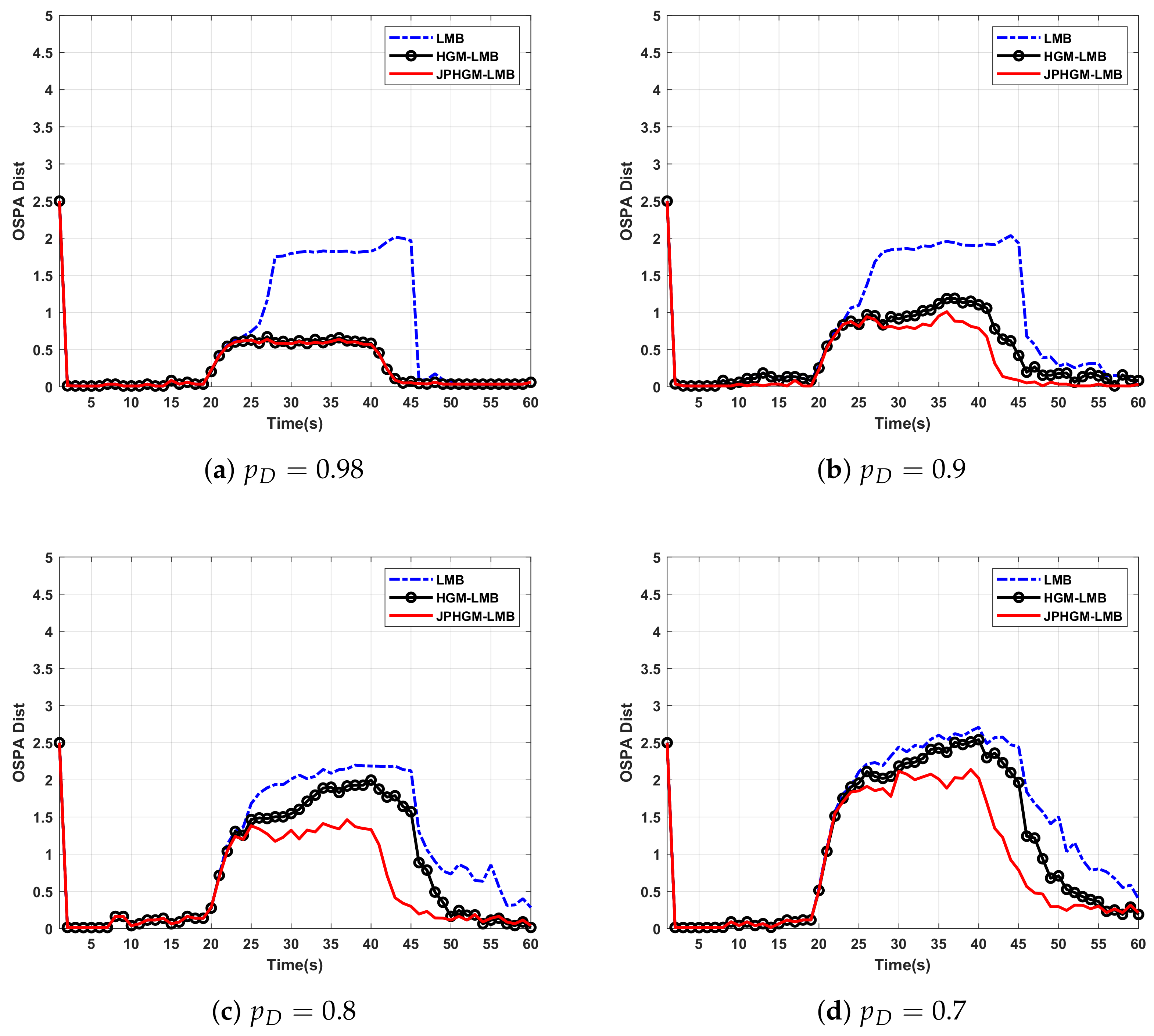
The effect of the turning rate $\omega$ and detection probability $p_D$ on the tracking performance is analyzed. Note that while analyzing the effect of one parameter, the other parameters remain unchanged. The OSPA of these filters with different detection probability $p_D$ and $\omega =3^{\circ }/\mathrm{s}$ are shown in Figure 6.

When targets maneuvering during the interval 20 s–40 s, there is a mismatch between actual motion model and dynamic motion model. Consequently, the estimation accuracy of target states degrades even if the data association is correct. Furthermore, it is susceptible to obtain wrong association results because of the model mismatching. From Figure 6, we can see that the OSPA distances of three filters increase when targets maneuvering. It can be observed that JPHGM-LMB filter outperforms HGM-LMB and LMB filter when the detection probability varies because not only the structure information of targets is used, but also all of the undetected cases are considered. However, the performance of JPHGM -LMB also degrades as detection probability decreases. The reason is that missed detections broken the structure of targets to some extent. An extreme case is that only one target is detected and thus no structure information can be used.

In order to further validate the superiority of JPHGM -LMB, clear mot metrics of these filters with different detection probability $p_D$ are shown in

Table 1. Clear mot metrics of filters with different detection probability.

		MOTP	Miss Rate	False Positive Rate	Mismatches	MOTA
	LMB	$\mathbf{0.166}$	$8.84\%$	$8.17\%$	$6.63$	$80.35\%$
$p_D=0.98$	HGM-LMB	$0.1892$	$1.36\%$	$0.69\%$	$0.64$	$97.68\%$
	JPHGM-LMB	$0.1901$	$\mathbf{1.34}\%$	$\mathbf{0.65}\%$	$\mathbf{0.04}$	$\mathbf{98}\%$
	LMB	$\mathbf{0.1562}$	$11.93\%$	$10.87\%$	$9.43$	$73.27\%$
$p_D=0.9$	HGM-LMB	$0.1753$	$5.94\%$	$4.75\%$	$2.92$	$88.09\%$
	JPHGM-LMB	$0.1797$	$\mathbf{4.2}\%$	$\mathbf{3.54}\%$	$\mathbf{0.95}$	$\mathbf{91.86}\%$
	LMB	$\mathbf{0.1467}$	$16.07\%$	$14.86\%$	$12.75$	$63.75\%$
$p_D=0.8$	HGM-LMB	$0.1525$	$12.4\%$	$11.05\%$	$8.54$	$72.98\%$
	JPHGM-LMB	$0.1654$	$\mathbf{8.56}\%$	$\mathbf{7.17}\%$	$\mathbf{4.35}$	$\mathbf{82.46}\%$
	LMB	$\mathbf{0.1281}$	$20.87\%$	$18.92\%$	$16.64$	$53.28\%$
$p_D=0.7$	HGM-LMB	$0.1312$	$18\%$	$15.74\%$	$13.35$	$60.7\%$
	JPHGM-LMB	$0.1407$	$\mathbf{14.33}\%$	$\mathbf{12.2}\%$	$\mathbf{11.55}$	$\mathbf{68.83}\%$

* MOTP is the multiple object tracking precision and MOTA is the multiple object tracking accuracy.

.

From Table 1, we can see that JPHGM-LMB achieves lower miss rate and false positive rate than HGM-LMB and LMB. The number of mismatches of JPHGM-LMB is less than other filters as detection probability varies. These results further demonstrate the effectiveness of the proposed method. However, it can be observed that LMB achieves smaller MOTP than other filters and MOTP of these filters decrease as detection probability decreases. The reason is that MOTP only takes the difference between true target states and estimated states into account when there is no mismatch. However, mismatches are more likely to happened when targets maneuvering and the estimation accuracy of target states degrades when target maneuvering as mentioned above.

The OSPA of these filters with different turning rate $\omega$ and $p_D=0.9$ are shown in Figure 7. From Figure 7, we can see that turning rate $\omega$ has significant effect on the performance of targets tracking, the tracking performance degrades a lot as the turning rate increases. Highly unreliable estimates are obtained with larger turning rate and appear in the OSPA curve. The larger the turning rate is, the more serious the model mismatch is. As mentioned above, the estimation accuracy of target states degrades even if the data association is correct when model is mismatched. If one target is undetected at one moment, there is no measurement available to update its prediction state which is obtained through preset dynamic motion model. Because of the model mismatch, the state estimates of this target will be far away from the true state, the more serious model mismatch is, the worse target state estimation is, the target may be eliminated if target state estimation is worse enough, then the targets cardinality will be underestimated. The structure of targets is destroyed in some degree, the state estimates of this target can converge to true state again after several time steps if it is detected, then the structure of targets can be recovered. The more time is needed with larger turning rate. If missed detection occurs again before the structure is restored, the structure of targets may be destroyed permanent, the poor performance of JPHGM-LMB and HGM-LMB will be achieved.

Clear mot metrics of these filters with different turning rate $\omega$ are in

Table 2. Clear mot metrics of filters with different turning rate.

		MOTP	Miss Rate	False Positive Rate	Mismatches	MOTA
	LMB	$\mathbf{0.0844}$	$1.97\%$	$0.8\%$	$1.13$	$96.75\%$
$\omega =1^{\circ }/\mathrm{s}$	HGM-LMB	$0.0851$	$1.5\%$	$0.31\%$	$0.3$	$98.07\%$
	JPHGM-LMB	$0.0852$	$\mathbf{0.95}\%$	$\mathbf{0.31}\%$	$\mathbf{0.12}$	$\mathbf{98.69}\%$
	LMB	$\mathbf{0.1562}$	$11.93\%$	$10.87\%$	$9.43$	$73.27\%$
$\omega =3^{\circ }/\mathrm{s}$	HGM-LMB	$0.1753$	$5.94\%$	$4.75\%$	$2.92$	$88.09\%$
	JPHGM-LMB	$0.1797$	$\mathbf{4.2}\%$	$\mathbf{3.54}\%$	$\mathbf{0.95}$	$\mathbf{91.86}\%$
	LMB	$\mathbf{0.2369}$	$14.11\%$	$12.65\%$	$13.13$	$67.77\%$
$\omega =5^{\circ }/\mathrm{s}$	HGM-LMB	$0.2379$	$10.81\%$	$9.32\%$	$9.59$	$75.88\%$
	JPHGM-LMB	$0.2664$	$\mathbf{5.89}\%$	$\mathbf{4.92}\%$	$\mathbf{6.51}$	$\mathbf{86.48}\%$
	LMB	$\mathbf{0.076}$	$39.35\%$	$29.65\%$	$18.52$	$23.28\%$
$\omega =8^{\circ }/\mathrm{s}$	HGM-LMB	$0.0847$	$35.39\%$	$22.55\%$	$16.74$	$35.08\%$
	JPHGM-LMB	$0.0938$	$\mathbf{32.6}\%$	$\mathbf{20.47}\%$	$\mathbf{13.5}$	$\mathbf{41.3}\%$

* MOTP is the multiple object tracking precision and MOTA is the multiple object tracking accuracy.

.

From Table 2, it is shown that larger turning rate leads to poor performance. The performance of these filters degrades dramatically with increasing turning rate. However, JPHGM-LMB always outperforms LMB and HGM-LMB as turning rate varies. The effectiveness of the proposed method is validated again.

The average computation time for tracking these four targets of three filter with $p_D=0.9$ is shown in Figure 8. As mentioned in Section 3, JPHGM-LMB follows some idea of JPDA, it suffers the problem of JPDA more or less, the number of association events grows exponentially with the number of targets. The better tracking performance is achieved at the sacrifice of computation time.

4.2. Scenario 2

In scenario 2, in order to further validate the superiority of proposed method, the proposed method is demonstrated on simulated data for multiple rigid targets. This scenario can be considered as the tracking of cars in urban traffic, there are more challenges in practice. On the one hand, because of an inherent property of many sensor types, such as laser and video, the sensors are subject to occlusions, the measurements are missed on successive time instants, the structures of targets are broken to some extent. On the other hand, the increasing of measurement errors lead to the deformation of the target’s structures, the effect of these factors will be analysed below. The birth and death of targets are considered in this scenario. Two rigid targets moving along different lines, the born time and end time of the first rigid target are $k=1$ and $k=50$ respectively, the target move along a straight line with a nearly constant velocity (CV) from 1 s to 20 s and follow a nearly constant acceleration (CA) model during the interval $20\mathrm{s}–40\mathrm{s}$ and move along a straight line with a nearly constant velocity (CV) during the interval $40\mathrm{s}–50\mathrm{s}$. The second rigid target born at $k=5$ and die at $k=55$, the target follow a nearly constant velocity (CV) during the interval $5\mathrm{s}–20\mathrm{s}$ and $40\mathrm{s}–55\mathrm{s}$, a nearly constant acceleration (CA) model is followed during the interval $20\mathrm{s}–40\mathrm{s}$. The surveillance region is $[-1000\mathrm{m},1000\mathrm{m}]\times [-1000\mathrm{m},1000\mathrm{m}]$, we set totally 60 time steps and the sampling time is 1 s.

The initial states of scattering centers of two rigid targets are given

$$\begin{array}{cc}\hfill {\mathit{x}}_0^{(1,1)}& =[-1000\mathrm{m},1010\mathrm{m},20\mathrm{m}/\mathrm{s},0\mathrm{m}/\mathrm{s}],t_s^{(1,1)}=1\mathrm{s},t_e^{(1,1)}=50\mathrm{s};\hfill \\ \hfill {\mathit{x}}_0^{(1,2)}& =[1000\mathrm{m},1000\mathrm{m},20\mathrm{m}/\mathrm{s},0\mathrm{m}/\mathrm{s}],t_s^{(1,2)}=1\mathrm{s},t_e^{(1,2)}=50\mathrm{s};\hfill \\ \hfill {\mathit{x}}_0^{(1,3)}& =[-995\mathrm{m},1011\mathrm{m},20\mathrm{m}/\mathrm{s},0\mathrm{m}/\mathrm{s}],t_s^{(1,3)}=1\mathrm{s},t_e^{(1,3)}=50\mathrm{s};\hfill \\ \hfill {\mathit{x}}_0^{(1,4)}& =[-995\mathrm{m},1007\mathrm{m},20\mathrm{m}/\mathrm{s},0\mathrm{m}/\mathrm{s}],t_s^{(1,4)}=1\mathrm{s},t_e^{(1,4)}=50\mathrm{s};\hfill \\ \hfill {\mathit{x}}_0^{(2,1)}& =[-1000\mathrm{m},-990\mathrm{m},20\mathrm{m}/\mathrm{s},0\mathrm{m}/\mathrm{s}],t_s^{(2,1)}=5\mathrm{s},t_e^{(2,1)}=55\mathrm{s};\hfill \\ \hfill {\mathit{x}}_0^{(2,2)}& =[-1000\mathrm{m},-1000\mathrm{m},20\mathrm{m}/\mathrm{s},0\mathrm{m}/\mathrm{s}],t_s^{(2,2)}=5\mathrm{s},t_e^{(2,2)}=55\mathrm{s};\hfill \\ \hfill {\mathit{x}}_0^{(2,3)}& =[-995\mathrm{m},-989\mathrm{m},20\mathrm{m}/\mathrm{s},0\mathrm{m}/\mathrm{s}],t_s^{(2,3)}=5\mathrm{s},t_e^{(2,3)}=55\mathrm{s};\hfill \\ \hfill {\mathit{x}}_0^{(2,4)}& =[-995\mathrm{m},-993\mathrm{m},20\mathrm{m}/\mathrm{s},0\mathrm{m}/\mathrm{s}],t_s^{(2,4)}=5\mathrm{s},t_e^{(2,4)}=55\mathrm{s};\hfill \end{array}$$

(48)

where ${\mathit{x}}_0^{(i,j)}$ is the initial state of $i\text{-}\mathrm{th}$ scattering center of $j\text{-}\mathrm{th}$ rigid target, $t_s^{(i,j)}$ is the born time of $i\text{-}\mathrm{th}$ scattering center of $j\text{-}\mathrm{th}$ rigid target, $t_e^{\left(i\right)}$ is the end time of $i\text{-}\mathrm{th}$ scattering center of $j\text{-}\mathrm{th}$ rigid target. The birth intensity in the simulation is

$$D_b\left(\mathit{\xi }\right)=\sum _{i=1}^2\sum _{j=1}^4{w}_b\mathcal{N}(\mathit{x};{\mathit{x}}_0^{(i,j)},{\mathbf{P}}_b),$$

(49)

where $w_b=0.03$, ${\mathbf{P}}_b=\mathrm{diag}\left([100,100,100,100]\right)$.

The true trajectories of these targets are shown in Figure 9.

In this section, the detection probability is $p_D=0.9$ and the acceleration of CA model is $\mathit{a}$ = 1.5 m/s².

Firstly, the effect of measurement errors on tracking performance is analyzed. The OSPA and clear mot metrics of these filters with different measurement errors are shown in Figure 10 and

Table 3. Clear mot metrics of filters with different measurement errors.

		MOTP	Miss Rate	False Positive Rate	Mismatches	MOTA
	LMB	$0.6266$	$7.5\%$	$6.62\%$	$50.66$	$73.28\%$
${\sigma }_m=0.1\mathrm{m}$	HGM-LMB	$0.4698$	$4.29\%$	$3.05\%$	$27.98$	$85.74\%$
	JPHGM-LMB	$\mathbf{0.4053}$	$\mathbf{3.23}\%$	$\mathbf{2.54}\%$	$\mathbf{23.52}$	$\mathbf{88.41}\%$
	LMB	$1.009$	$10.56\%$	$9.18\%$	$60.58$	$63.9\%$
${\sigma }_m=0.2\mathrm{m}$	HGM-LMB	$0.9432$	$8.41\%$	$6.94\%$	$58.7$	$70.13\%$
	JPHGM-LMB	$\mathbf{0.7436}$	$\mathbf{5.03}\%$	$\mathbf{4.27}\%$	$\mathbf{48.82}$	$\mathbf{78.61}\%$
	LMB	$1.11$	$12.54\%$	$11.12\%$	$63.52$	$60.61\%$
${\sigma }_m=0.3\mathrm{m}$	HGM-LMB	$1.01$	$11.3\%$	$9.33\%$	$59.36$	$63.25\%$
	JPHGM-LMB	$\mathbf{0.8985}$	$\mathbf{9.45}\%$	$\mathbf{7.64}\%$	$\mathbf{52.08}$	$\mathbf{68.79}\%$
	LMB	$1.1745$	$14.75\%$	$13.82\%$	$66.1$	$56.44\%$
${\sigma }_m=0.4\mathrm{m}$	HGM-LMB	$1.0519$	$14.45\%$	$12.32\%$	$65.14$	$58.78\%$
	JPHGM-LMB	$\mathbf{1.016}$	$\mathbf{13.96}\%$	$\mathbf{12.2}\%$	$\mathbf{57.48}$	$\mathbf{60.54}\%$

* MOTP is the multiple object tracking precision and MOTA is the multiple object tracking accuracy.

respectively.

From Figure 10, when targets maneuvering during the interval 20 s–40 s, the OSPA of three filters increases, the reason is the mismatch between actual motion model and dynamic motion model. When targets born or die, the number of targets will change, these filters will take some time to obtain the true number of targets, then the OSPA distance increase. The performance of JPHGM-LMB degrades with increasing measurement error and these filters achieves almost similar performance when ${\sigma }_m=0.4\mathrm{m}$. However, JPHGM-LMB outperforms other filters, because JPHGM-LMB takes both kinematic and structure information into account and missed detections are considered. In JPHGM-LMB, the hypergraph is introduced to represent the structure of predictions and measurements, then the problem of data association can be formulated as a hypergraph matching problem, it becomes more challenge to obtain the correct matching results as measurement errors increases. Moreover, the structure of targets will be deformed because unreliable measurements are used to update the states of targets. From Table 3, JPHGM-LMB achieves larger MOTA values than other filters, it means that JPHGM-LMB obtains higher quality trajectories than other filters, it further validates the superiority of JPHGM-LMB.

Secondly, the effect of occlusions are considered, it can not be avoided in practice applications, for example, the car may be partly covered by pedestrians or other barriers. In order to simulate occlusions, the $4\mathrm{th}$ scattering centers of two rigid targets are occluded during several time steps for simplicity. The beginning of the occlusion is at $k=32\mathrm{s}$ (targets are maneuvering), the duration of occlusion is denoted by $\beta$. The OSPA and clear mot metrics of these filters with different occlusion time steps are shown in Figure 11 and

Table 4. Clear mot metrics of filters with different occlusion duration.

		MOTP	Miss Rate	False Positive Rate	Mismatches	MOTA
	LMB	$0.6484$	$7.64\%$	$7.05\%$	53	$72.19\%$
$\beta =1\mathrm{s}$	HGM-LMB	$0.5029$	$4.74\%$	$3.83\%$	$33.22$	$83.2\%$
	JPHGM-LMB	$\mathbf{0.4119}$	$\mathbf{3.51}\%$	$\mathbf{2.98}\%$	$\mathbf{27.04}$	$\mathbf{86.82}\%$
	LMB	$0.6102$	$7.83\%$	$6.46\%$	$50.54$	$73.21\%$
$\beta =2\mathrm{s}$	HGM-LMB	$0.4741$	$6.21\%$	$4.14\%$	$32.02$	$81.72\%$
	JPHGM-LMB	$\mathbf{0.3893}$	$\mathbf{4.66}\%$	$\mathbf{3.13}\%$	$\mathbf{25.34}$	$\mathbf{85.94}\%$
	LMB	$0.5618$	$8.9\%$	$5.39\%$	$47.3$	$74.01\%$
$\beta =3\mathrm{s}$	HGM-LMB	$0.4497$	$8.28\%$	$3.52\%$	$31.16$	$80.49\%$
	JPHGM-LMB	$\mathbf{0.3802}$	$\mathbf{7.34}\%$	$\mathbf{3.48}\%$	$\mathbf{24.38}$	$\mathbf{83.15}\%$
	LMB	$0.5472$	$10.71\%$	$4.73\%$	$43.66$	$73.76\%$
$\beta =4\mathrm{s}$	HGM-LMB	$0.433$	$11.14\%$	$3.14\%$	$29.42$	$78.44\%$
	JPHGM-LMB	$\mathbf{0.3814}$	$\mathbf{10.31}\%$	$\mathbf{3.01}\%$	$\mathbf{22.96}$	$\mathbf{81.03}\%$

* MOTP is the multiple object tracking precision and MOTA is the multiple object tracking accuracy.

respectively.

When occlusion happened, there are two aspects. Firstly, the number of targets will be underestimated, filters take several time steps to obtain the true cardinality estimation. There is no measurement available to update prediction state of occluded target, the estimation error of occluded target can not be avoided because of the model mismatch and measurement noise, the OSPA distance increases as shown in Figure 11. However, the superiority of JPHGM-LMB can be found clearly in Table 4, JPHGM-LMB always achieves larger MOTA than other filters as occlusion duration increases. Secondly, the structure of targets is broken to some extent when occlusion happened, the structure can be recovered if occlusion duration is short, then the structure information can also enhance the tracking performance, see Figure 11a,b. However, if occlusion duration is long enough, then the structure of targets may be destroyed permanent, the performance of HGM-LMB and JPHGM-LMB will degrade, see Figure 11c,d.

5. Conclusions

In this paper, hypergraph representation is adopted to incorporate structure information of rigid targets for better data association performance in MTT. The problem of data association is formulated as a hypergraph matching problem. To achieve better data association performance in hostile environments with clutter and missed detections, all undetected cases are enumerated following some ideas of joint probabilistic data association and the likelihood is built based on group structure rather than distance between predicted states and measurements. Then, the structure information is integrated into LMB filter by revising each single target likelihood with joint association probabilities. However, the number of association events grows exponentially with the number of targets, the proposed approach is usable in real time only for a limited number of targets. The effectiveness of our method has been demonstrated by extensive experiments. Specially, in the first scenario, when detection probability is 0.9, MOTA of JPHGM-LMB is $91.86\%$, there is almost three percent increase compared with HGM-LMB and eight percent increase compared with LMB. Moreover, as detection probability decreases, JPHGM-LMB always outperforms other filters. In the second scenario, when the standard deviation of measurement noise is 0.2 m, MOTA of JPHGM-LMB achieves $78.61\%$, however, that of HGM-LMB and LMB are $70.13\%$ and $63.9\%$ respectively, JPHGM-LMB achieves better tracking performance.

The representation of hypergraph can utilize the structure information well, it can handle camera shake, because the structure of targets remain unchanged, the measurement noise will be more complicated if camera shake is considered. In order to handle more complex scenarios in practice applications, particle filter may be introduced, then the problem is how to reduce computational cost, it is our future work.

References

Ding, Y.; Yu, X.; Zhang, J.; Xu, X. Application of Linear Predictive Coding and Data Fusion Process for Target Tracking by Doppler Through-Wall Radar. IEEE Trans. Microw. Theory Tech.2019, 67, 1–11. [Google Scholar] [CrossRef]
Zhang, Y.; Mu, H.; Jiang, Y.; Ding, C.; Wang, Y. Moving Target Tracking Based on Improved GMPHD Filter in Circular SAR System. IEEE Geosci. Remote Sens. Lett.2019, 16, 559–563. [Google Scholar] [CrossRef]
Clark, D.E.; Bell, J. Bayesian multiple target tracking in forward scan sonar images using the PHD filter. IEEE Radar Sonar Navig.2005, 152, 327–334. [Google Scholar] [CrossRef] [Green Version]
Cox, L.J.; Hingorani, S.L. An efficient implementation of Reid’s multiple hypothesis tracking algorithm and its evaluation for the purpose of visual tracking. IEEE Trans. Pami1996, 2, 437–442. [Google Scholar] [CrossRef] [Green Version]
Mullane, J.; Vo, B.N.; Adams, M.; Vo, B.T. A Random-Finite-Set Approach to Bayesian SLAM. IEEE Trans. Robot.2011, 27, 268–282. [Google Scholar] [CrossRef]
Blackman, S.; Popoli, R. Design and Analysis of Modern Tracking Systems; Artech House: Norwood, MA, USA, 1999. [Google Scholar]
Barshalom, Y. Multitarget-Multisensor Tracking: Aplications and Advances; Artech House: Norwood, MA, USA, 1993. [Google Scholar]
Bar-Shalom, Y.; Willett, P.K.; Tian, X. Tracking and Data Fusion: A Handbook of Algorithms; YBS Publishing: Storrs, CT, USA, 2011. [Google Scholar]
Reid, D.B. An Algorithm for Tracking Multiple Targets. IEEE Trans. Autom. Control1979, 24, 1202–1211. [Google Scholar] [CrossRef]
Mahler, R. Statistical Multisource-Multitarget Information Fusion; Artech House: Norwood, MA, USA, 2007. [Google Scholar]
Mahler, R. Advances in Statistical Multisource-Multitarget Information Fusion; Artech House: Norwood, MA, USA, 2014. [Google Scholar]
Musicki, D.; Evans, R. Joint Integrated Probabilistic Data Association: JIPDA. IEEE Trans. Aerosp. Electron. Syst.2004, 40, 1093–1099. [Google Scholar] [CrossRef]
Sastry, S.O.R. Markov Chain Monte Carlo Data Association for Multi-Target Tracking. IEEE Trans. Autom. Control2009, 54, 481–497. [Google Scholar]
Williams, J.; Lau, R. Approximate evaluation of marginal association probabilities with belief propagation. IEEE Trans. Aerosp. Electron. Syst.2014, 50, 2942–2959. [Google Scholar] [CrossRef] [Green Version]
Williams, J.L.; Lau, R.A. Multiple scan data association by convex variational inference. IEEE Trans. Signal Process.2018, 66, 2112–2127. [Google Scholar] [CrossRef] [Green Version]
Xie, X.; Evans, R.J. Multiple target tracking and multiple frequency line tracking using hidden Markov models. IEEE Trans. Signal Process.1991, 39, 2659–2676. [Google Scholar] [CrossRef]
Ruan, Y.; Willett, P. The turbo PMHT. IEEE Trans. Aerosp. Electron. Syst.2004, 40, 1388–1398. [Google Scholar] [CrossRef]
Brekke, E.; Chitre, M. Relationship between Finite Set Statistics and the Multiple Hypothesis Tracker. IEEE Trans. Aerosp. Electron. Syst.2018, 54, 1902–1917. [Google Scholar] [CrossRef]
Mahler, R. PHD filters of higher order in target number. IEEE Trans. Aerosp. Electron. Syst.2008, 43, 1523–1543. [Google Scholar] [CrossRef]
Vo, B.T.; Vo, B.N.; Cantoni, A. The Cardinality Balanced Multi-Target Multi-Bernoulli Filter and Its Implementations. IEEE Trans. Signal Process.2009, 57, 409–423. [Google Scholar]
Vo, B.N.; Vo, B.T.; Pham, N.T.; Suter, D. Joint Detection and Estimation of Multiple Objects From Image Observations. IEEE Trans. Signal Process.2010, 58, 5129–5141. [Google Scholar] [CrossRef]
Vo, B.T.; Vo, B.N. Labeled Random Finite Sets and Multi-Object Conjugate Priors. IEEE Trans. Signal Process.2013, 61, 3460–3475. [Google Scholar] [CrossRef]
Vo, B.T.; Vo, B.N.; Phung, D. Labeled Random Finite Sets and the Bayes Multi-Target Tracking Filter. IEEE Trans. Signal Process.2014, 62, 6554–6567. [Google Scholar] [CrossRef] [Green Version]
Reuter, S.; Vo, B.T.; Vo, B.N.; Dietmayer, K. The Labeled Multi-Bernoulli Filter. IEEE Trans. Signal Process.2014, 62, 3246–3260. [Google Scholar]
Hammarstrand, L.; Lundgren, M.; Svensson, L. Adaptive Radar Sensor Model for Tracking Structured Extended Objects. IEEE Trans. Aerosp. Electron. Syst.2012, 48, 1975–1995. [Google Scholar] [CrossRef] [Green Version]
Wu, S.; Hong, L.; Layne, J.R. 2D rigid-body target modelling for tracking and identification with GMTI/HRR measurements. IEE Control Theory Appl.2004, 151, 429–438. [Google Scholar] [CrossRef]
Wu, S.; Xiao, J. Tracking group targets using hypergraph matching in data association. In Proceedings of the SPIE Conference on Signal and Data Processing of Small Targets, San Diego, CA, USA, 15–18 September 2011; pp. 1–9. [Google Scholar]
Yu, H.; An, W.; Zhu, R.; Guo, R. A Hypergraph Matching Labeled Multi-Bernoulli Filter for Group Targets Tracking. IEICE Trans. Inf. Syst.2019, 102, 2077–2081. [Google Scholar] [CrossRef]
Bailey, T.; Nebot, E.M.; Rosenblatt, J.K.; Durrant-Whyte, H.F. Data Association for Mobile Robot Navigation: A Graph Theoretic Approach. In Proceedings of the IEEE International Conference on Robotics and Automation, San Francisco, CA, USA, 24–28 April 2000; pp. 2512–2517. [Google Scholar]
Zass, R.; Shashua, A. Probabilistic graph and hypergraph matching. In Proceedings of the IEEE Conference on Computer Vision and Pattern Recognition, Anchorage, AK, USA, 23–28 June 2008; pp. 1–8. [Google Scholar]
Cho, M.; Lee, J.; Lee, K.M. Reweighted Random Walks for Graph Matching. In Proceedings of the European Conference on Computer Vision, Heraklion, Crete, Greece, 5–11 September 2010; pp. 492–505. [Google Scholar]
Schuhmacher, D.; Vo, B.T.; Vo, B.N. A consistent metric for performance evaluation of multi-object filters. IEEE Trans. Signal Process.2008, 56, 3447–3457. [Google Scholar] [CrossRef] [Green Version]
Bernardin, K.; Stiefelhagen, R. Evaluating Multiple Object Tracking Performance: The CLEAR MOT Metrics. EURASIP J. Image Video Process.2008, 2008, 1–10. [Google Scholar] [CrossRef] [Green Version]
Figure 1.
Sketch of hypergraph matching: (a) idea situation and (b) hostile situation.
Figure 2.
True trajectories of four targets.
Figure 3.
Trajectories obtained by three filters: (a) LMB, (b) HGM-LMB and (c) JPHGM-LMB.
Figure 4.
Data association results of LMB and JPHGM-LMB: (a) LMB and (b) JPHGM-LMB.
Figure 5.
Data association results of HGM-LMB and JPHGM-LMB: (a) HGM-LMB and (b) JPHGM-LMB.
Figure 6.
The OSPA of three filters with different detection probability: (a) , (b) , (c) and (d) .
Figure 7.
The OSPA of three filters with different turning rate: (a) , (b) , (c) and (d) .
Figure 8.
The average computation time for these filters.
Figure 9.
True trajectories in scenario 2.
Figure 10.
The OSPA of three filters with different measurement errors: (a) , (b) , (c) and (d) .
Figure 11.
The OSPA of three filters with different occlusion duration: (a) , (b) , (c) and (d) .