An Adaptive Target Tracking Algorithm Based on EKF for AUV with Unknown Non-Gaussian Process Noise

Abstract

An adaptive target tracking method based on extended Kalman filter (TT-EKF) is proposed to simultaneously estimate the state of an Autonomous Underwater Vehicle (AUV) and an mobile recovery system (MRS) with unknown non-Gaussian process noise in homing process. In the application scenario of this article, the process noise includes the measurement noise of AUV heading and forward speed and the estimation error of MRS heading and forward speed. The accuracy of process noise covariance matrix (PNCM) can affect the state estimation performance of the TT-EKF. The variational Bayesian based algorithm is applied to estimate the process noise statistics. We use a Gaussian mixture distribution to model the non-Gaussian noisy forward speed of AUV and MRS. We use a von-Mises distribution to model the noisy heading of AUV and MRS. The variational Bayesian algorithm is applied to estimate the parameters of these distributions, and then the PNCM can be calculated. The prediction error of TT-EKF is online compensated by using a multilayer neural network, and the neural network is online trained during the target tracking process. Matlab simulation and experimental data analysis results verify the effectiveness of the proposed method.

1. Introduction

For target tracking in the ocean environment, two approaches are generally used. Linear Kalman filter (KF) is a first and foremost approach, and the extended Kalman filter(EKF) is the second approach [1,2,3,4,5]. KF/EKF is highly sensitive to the accuracy of the noise statistics. In practical applications, as is often the case, the covariance matrixes of the process noise and the measurement noise may be unknown or inaccurate. In the case of unknown covariance matrixes, the state estimation performance of KF/EKF will be decreased and it may even diverge [6]. More and more adaptive filters with model uncertainty are developed to solve this problem. In this manuscript, we focus on the model uncertainty of the process noise, specifically, the process noise is unknown and non-Gaussian.

A variety of filters were proposed to address the state estimation problem with unknown noise covariance matrixes, such as robust KF [7,8], adaptive KF [9,10,11,12,13,14,15], and others [16]. Generally Speaking, the adaptive KF methods can be divided into covariance matching, maximum likelihood (ML), Bayesian methods and so on. More recently, the variational Bayesian (VB) methods wasn applied into the filtering framework [17,18,19]. In [14,20], a VB adaptive KF are proposed to jointly estimate the state and the measurement noise covariance matrix (MNCM) where the prior distribution of the covariance is governed by an inverse-Gamma distribution and inverse-Wishart distribution, respectively.

To the best of our knowledge, the VB-based adaptive filters are only used for online state estimation with unknown MNCM, and rarely used for the online state estimation with unknown process noise covariance matrix (PNCM). In [13], the online state estimation with inaccurate PNCM is treated, in which the prediction error covariance matrix rather than PNCM is approximated by the VB method. It cannot give the estimated value of the unknown PNCM. Besides, the authors of [21] experimentally show that the state estimation performance of the proposed adaptive filter in [13] may be worse than that of the traditional KF in some cases. In [22], a new adaptive KF algorithm is proposed to cope with the unknown PNCM for the linear discrete-time systems. The PNCM is estimated by the proposed algorithm based on the measurement sequence. In [23], an adaptive KF algorithm in presence of PNCM based on black box variational inference is proposed. The black box variational inference method is recently introduced to conduct the approximate Bayesian inference for the non-conjugate probabilistic model. They structured a posterior model of the system state and PNCM firstly, and then, the black box variational inference online inference for the posterior distribution of the PNCM is derived.

In this paper, we address the online state estimation problem in the presence of the unknown and non-Gaussian PNCM. For the target tracking in the ocean environment, the process noise of AUV is unknown or inaccurate, and the process noise of MRS is unknown totally. Due to the complexity of an underwater environment, the actual noise of AUV speed sensor is non-Gaussian. The main contributions of this paper are summarized as follows:

• We propose a target tracking method based on EKF (TT-EKF) to simultaneously estimate the states of an AUV and an MRS.
• We estimate the noise statistics of the heading and forward speed of an AUV and an MRS by using the variational Bayesian algorithm. The noisy forward speed is modeled by the Gaussian mixture distribution (GMD). The noisy heading angle is modeled by a von Mises (vM) distribution.
• We build a neural network compensator to make up for the prediction error caused by the process noise.

2. System Overview

In this section, we introduce an AUV and a mobile recovery system, which are illustrated in Figure 1. The MRS includes an AUV (is called AUV-I) and a docking station. The docking station was rigidly fixed to the underbelly of AUV-I. The entrance of the docking station was a funnel-like, 2 m in diameter. The AUV to be recovered is called AUV-$II$. AUV-$II$ was a torpedo-shaped vehicle that was 384 mm in diameter and 5486 mm in length. It was equipped with a GPS, an inertial measurement unit (IMU), a Doppler velocity log (DVL) and an acoustic sensor. The acoustic sensor, Evologics 32C R, was used for long-range positioning. The AUV-I carries a transponder, and AUV-$II$ carries transceiver. The application scenario is: The MRS is moved with constant velocity and travels in a straight path, the AUV chases MRS to complete the homing process. The line-of-sight guidance algorithm is used to guide AUV to MRS.

Figure 1. An AUV to be recovered (a) and the mobile recovery system (b).

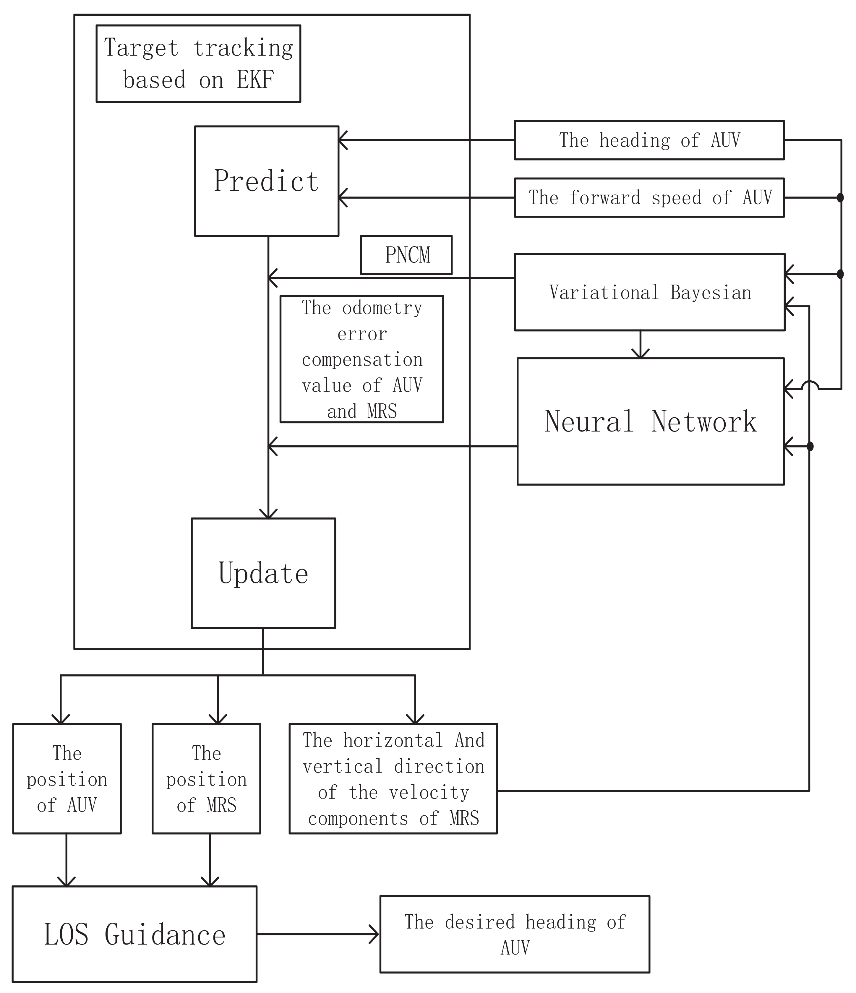
The AUV estimates the states of AUV and MRS based on TT-EKF with its own heading and forward speed. To estimate the PNCM, we model the heading and forward speed of AUV and MRS, and calculate the parameters of these distributions. The neural network is applied to compensate the prediction error. The framework of our proposed algorithm is shown in Figure 2.

Figure 2. The overview of our algorithm.

3. Target Tracking Method Based on EKF

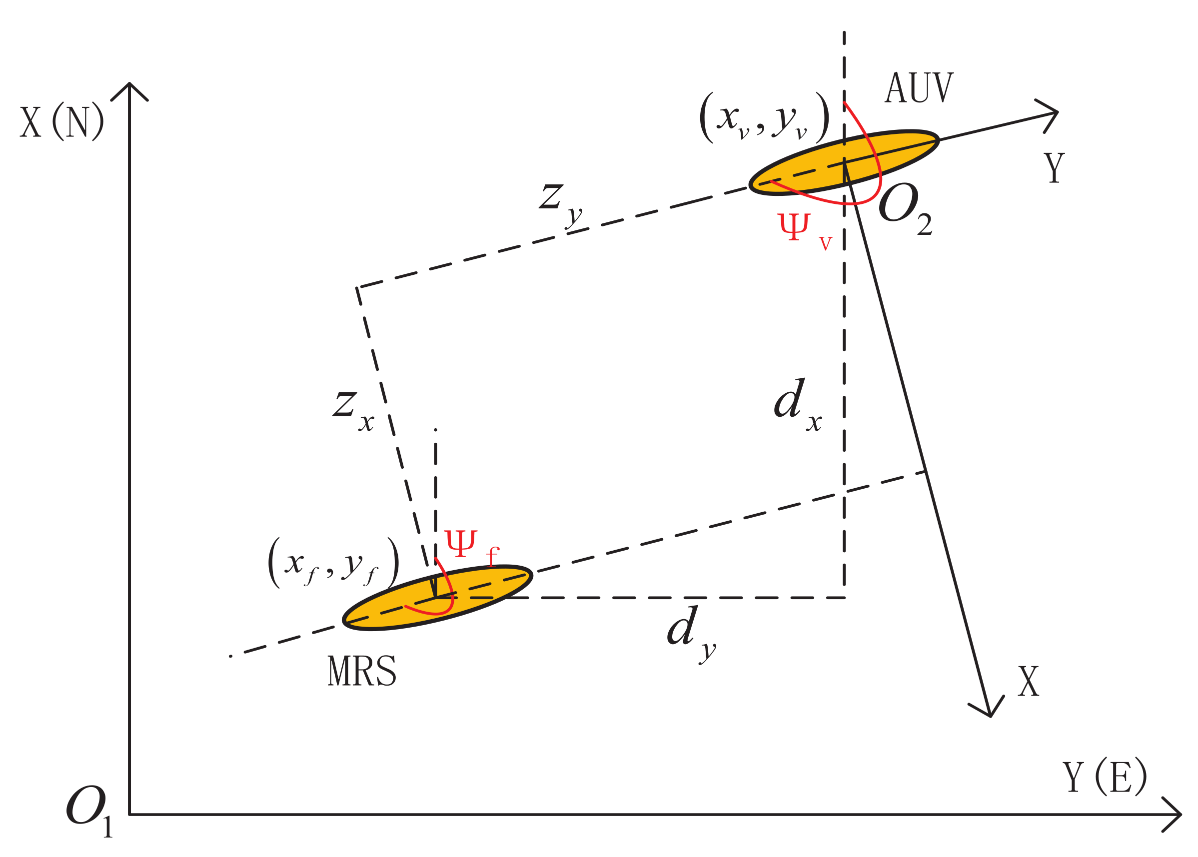
In this scenario, the AUV tracks MRS with the acoustic sensor, which measures the position of MRS in the AUV coordinate frame. The state of the target motion model is described by a nearly constant velocity model and at time step (k) includes the position in two dimensional (2D) Cartesian coordinates x and y and the velocity towards those coordinates axes $v_x$ and $v_y$. All coordinate frames are shown in Figure 3.

Figure 3. Coordinate frames schematic diagram.

In Figure 3, $\left(x_v,y_v\right)$ and ${\psi }_v$ are the position and heading of AUV, respectively. $\left(x_f,y_f\right)$ and ${\psi }_f$ are the position and heading of MRS, respectively. $O_1$ is the global North, East coordinate frame, $O_2$ is the local AUV coordinate frame. The measurement at time index k can be expressed as: $z_k={\left[z_x{z}_y\right]}^T$. $z_x$ and $z_y$ are the horizontal and vertical direction of the measurement components in $O_2$ local coordinate system. $d_x$ and $d_y$ are the horizontal and vertical direction of relative distance components between the AUV and MRS in global coordinate frame. The system state Cartesian coordinates is defined as follow:

$${\mathit{x}}_k={\left[x_{v,k}{y}_{v,k}{x}_{f,k}{\dot{x}}_{f,k}{y}_{f,k}{\dot{y}}_{f,k}\right]}^T$$

(1)

where ${\mathit{x}}_k$ is the system state at time index k, $x_{v,k}$ and $y_{v,k}$ are the Cartesian coordinates of AUV, $x_{f,k}$ and $y_{f,k}$ are the Cartesian coordinates of MRS, ${\dot{x}}_{f,k}$ and ${\dot{y}}_{f,k}$ are the horizontal and vertical direction of the forward speed components of MRS in $O_1$ global coordinate frame. The state transition model is:

$${\mathit{x}}_k=\mathit{F}·{\mathit{x}}_{k-1}+{\mathit{B}}_k+{\mathsf{\Gamma }}_k·{\mathit{w}}_k$$

(2)

where $\mathit{F}=\left[\begin{array}{cccccc}1& 0& 0& 0& 0& 0\\ 0& 1& 0& 0& 0& 0\\ 0& 0& 1& dt& 0& 0\\ 0& 0& 0& 1& 0& 0\\ 0& 0& 0& 0& 1& dt\\ 0& 0& 0& 0& 0& 1\end{array}\right]$, ${\mathit{B}}_k=\left[\begin{array}{c}{u}_{v,k}·cos\left({\psi }_{v,k}\right)·dt\\ u_{v,k}·sin\left({\psi }_{v,k}\right)·d\\ 0\\ 0\\ 0\\ 0\end{array}\right]$, ${\mathsf{\Gamma }}_k=\left[\begin{array}{cccc}cos\left({\psi }_{v,k}\right)·dt& -u_{v,k}·sin\left({\psi }_{v,k}\right)·dt& 0& 0\\ sin\left({\psi }_{v,k}\right)·dt& -u_{v,k}·cos\left({\psi }_{v,k}\right)·dt& 0& 0\\ 0& 0& cos\left({\psi }_{f,k}\right)·dt& u_{f,k}·sin\left({\psi }_{f,k}\right)·dt\\ 0& 0& cos\left({\psi }_{f,k}\right)& -u_{f,k}·sin\left({\psi }_{f,k}\right)\\ 0& 0& sin\left({\psi }_{f,k}\right)·dt& u_{f,k}·cos\left({\psi }_{f,k}\right)·dt\\ 0& 0& sin\left({\psi }_{f,k}\right)& u_{f,k}·cos\left({\psi }_{f,k}\right)\end{array}\right]$, $dt=t_k-t_{k-1}$. $u_{v,k}$ is the forward speed of AUV at time index k, ${\psi }_{v,k}$ is the heading of AUV at time index k. $u_{f,k}$ is the forward speed of MRS at time index k, ${\psi }_{f,k}$ is the heading of MRS at time index k. $w_k$ is process noise which is assumed to be zero mean non-Gaussian noise, and its covariance is a fourth-order square matrix. The covariance of process noise is $\mathit{Q}=\left[\begin{array}{cccc}Q\left(u_v\right)& 0& 0& 0\\ 0& Q\left({\psi }_v\right)& 0& 0\\ 0& 0& Q\left(u_f\right)& 0\\ 0& 0& 0& Q\left({\psi }_f\right)\end{array}\right]$, where $Q\left(u_v\right)$ is the noise variance of AUV speed, $Q\left({\psi }_v\right)$ is the noise variance of AUV heading, $Q\left(u_f\right)$ is the noise variance of MRS speed, $Q\left({\psi }_f\right)$ is the noise variance of MRS heading. The MRS is tracked by an acoustic sensor in the underwater and provides measurements of the position of MRS in the AUV coordinate frame.

The measurement model is given as

$$\begin{array}{c}{\mathit{z}}_k=h\left({\mathit{x}}_k\right)+{\mathit{v}}_k\end{array}$$

(3)

$$\begin{array}{c}h\left({\mathit{x}}_k\right)=\left[\begin{array}{c}-\left({\mathit{x}}_k\left(1,1\right)-{\mathit{x}}_k\left(3,1\right)\right)·sin\left({\psi }_{v,k}\right)+\left({\mathit{x}}_k\left(2,1\right)-{\mathit{x}}_k\left(5,1\right)\right)·cos\left({\psi }_{v,k}\right)\\ \left({\mathit{x}}_k\left(1,1\right)-{\mathit{x}}_k\left(3,1\right)\right)·cos\left({\psi }_{v,k}\right)+\left({\mathit{x}}_k\left(2,1\right)-{\mathit{x}}_k\left(5,1\right)\right)·sin\left({\psi }_{v,k}\right)\end{array}\right]\end{array}$$

(4)

where ${\mathit{v}}_k$ is uncorrelated, zero-mean white Gaussian noise with known second order covariance matrix. The measurement noise covariance maxtrix is denoted as $\mathit{R}$. The target tracking algorithm based on EKF is described as follows:

$$\begin{array}{c}{\mathit{x}}_k^{-}=\mathit{F}·{\mathit{x}}_{k-1}+{\mathit{B}}_k+{\mathsf{\Gamma }}_k·{\mathit{w}}_k\end{array}$$

(5)

$$\begin{array}{c}{\mathit{P}}_k^{-}={\mathit{F}}_k·{\mathit{P}}_{k-1}·{\mathit{F}}_k^T+{\mathsf{\Gamma }}_k·\mathit{Q}·{\mathsf{\Gamma }}_k^T\end{array}$$

(6)

$$\begin{array}{c}{\widehat{\mathit{z}}}_k=h\left({\mathit{x}}_k^{-}\right)\end{array}$$

(7)

$$\begin{array}{c}{\mathit{S}}_k={\mathit{H}}_k·{\mathit{P}}_k^{-}·{\mathit{H}}_k^T+\mathit{R}\end{array}$$

(8)

$$\begin{array}{c}{\mathit{K}}_k={\mathit{P}}_k^{-}·{\mathit{H}}_k^T·{\mathit{S}}_k^{-1}\end{array}$$

(9)

$$\begin{array}{c}{\mathit{x}}_k={\mathit{x}}_k^{-}+{\mathit{K}}_k·\left({\mathit{z}}_k-{\widehat{\mathit{z}}}_k\right)\end{array}$$

(10)

$$\begin{array}{c}{\mathit{P}}_k=\left(\mathit{I}-{\mathit{K}}_k·\mathit{H}\right)·{\mathit{P}}_k^{-}\end{array}$$

(11)

where $\mathit{F},{\mathit{B}}_k,{\mathsf{\Gamma }}_k,{\mathit{w}}_k,\mathit{Q},\mathit{R}$ have mentioned above. ${\mathit{x}}_{k-1}$ and ${\mathit{P}}_{k-1}$ are the state estimate and state covariance matrix at time index $k-1$, respectively. ${\mathit{x}}_k^{-}$ and ${\mathit{P}}_k^{-}$ are the prediction state estimate and prediction state covariance matrix at time index k, respectively. ${\mathit{x}}_k$ and ${\mathit{P}}_k$ are the updated state estimate and updated state covariance matrix at time index k, respectively. ${\widehat{\mathit{z}}}_k$ and ${\mathit{z}}_k$ are the predicted measurement and actual measurement at time index k, respectively. ${\mathit{K}}_k$ is the filter gain at time index k. ${\mathit{S}}_k$ is an auxiliary variable. $h\left(·\right)$ is measurement model and $\mathit{H}$ is measurement matrix, which is given by:

$${\mathit{H}}_k=\left[\begin{array}{cccccc}-cos\left({\psi }_{v,k}\right)& -sin\left({\psi }_{v,k}\right)& cos\left({\psi }_{v,k}\right)& 0& sin\left({\psi }_{v,k}\right)& 0\\ -sin\left({\psi }_{v,k}\right)& cos\left({\psi }_{v,k}\right)& sin\left({\psi }_{v,k}\right)& 0& -cos\left({\psi }_{v,k}\right)& 0\end{array}\right]$$

(12)

According to the state vector ${\mathit{x}}_k$, we can calculate the forward speed and heading of MRS at time index k.

$$\begin{array}{c}{u}_{f,k}=\sqrt{{\mathit{x}}_k{\left(4,1\right)}^2+{\mathit{x}}_k{\left(6,1\right)}^2}\end{array}$$

(13)

$$\begin{array}{c}{\psi }_{f,k}=\left\{\begin{array}{c}acos\left(\frac{{\mathit{x}}_k\left(4,1\right)}{\sqrt{{\mathit{x}}_k{\left(4,1\right)}^2+{\mathit{x}}_k{\left(6,1\right)}^2}}\right)if\frac{{\mathit{x}}_k\left(6,1\right)}{\sqrt{{\mathit{x}}_k{\left(6,1\right)}^2+{\mathit{x}}_k{\left(6,1\right)}^2}}>0\\ 2\pi -acos\left(\frac{{\mathit{x}}_k\left(4,1\right)}{\sqrt{{\mathit{x}}_k{\left(4,1\right)}^2+{\mathit{x}}_k{\left(6,1\right)}^2}}\right)else\end{array}\right.\end{array}$$

(14)

4. Adaptive Target Tracking Algorithm Based on EKF

For the application scenarios in this paper, the forward speed and heading of MRS are unknown. The noise statistics of forward speed and heading of AUV and MRS are unknown. It is assumed that the measurement noise statistics are Gaussian and known. The adaptive TT-EKF is applied to simultaneously estimate the position of AUV and MRS and the horizontal and vertical direction of the velocity components of MRS with unknown PNCM.

The structure of proposed adaptive target tracking algorithm is shown in Figure 4. In the algorithm, Variational Bayesian algorithm is used to estimate the PNCM. A multilayer neural network which acts as a feedforward error compensator is embedded in target tracking system to deal with the prediction errors caused by the noisy input vector.

Figure 4. Structure of proposed adaptive target tracking algorithm based on EKF.

5. Variational Bayesian

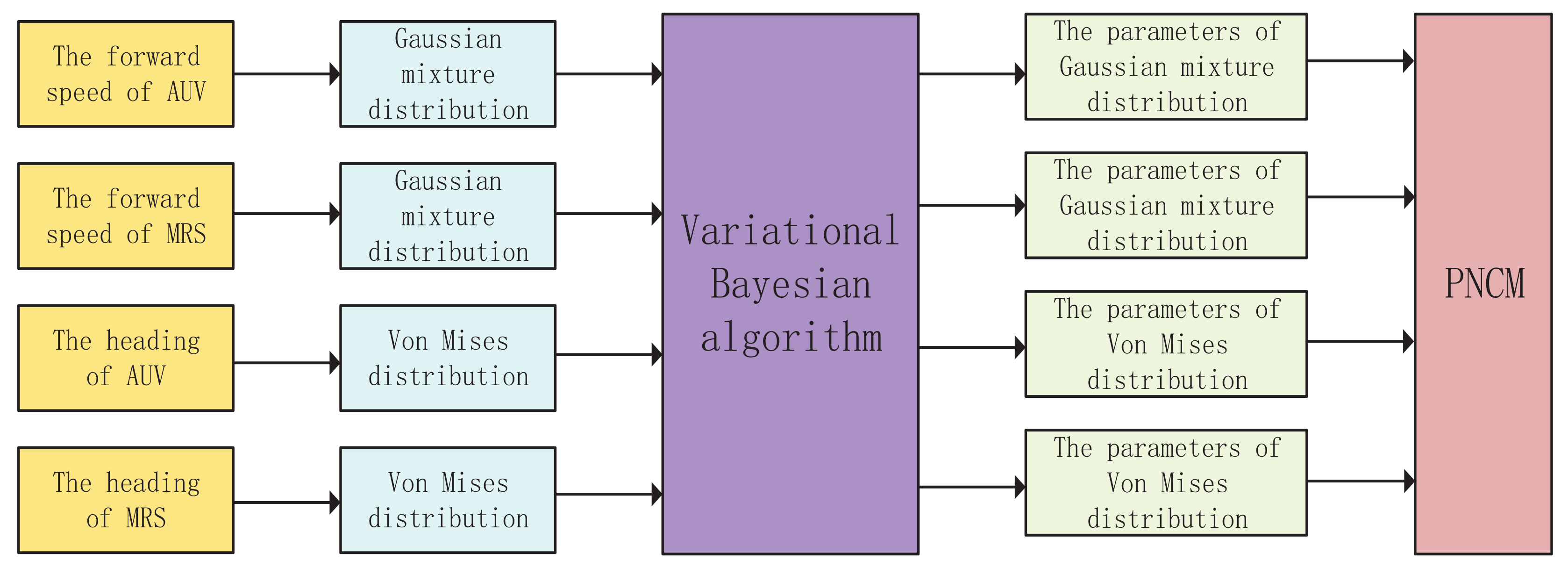
The forward speed of AUV is non-Gaussian due to the non-Gaussian process noise. The heading angle is a periodic variable. The probability distribution of forward speed and heading is modeled in Section 5.1. The parameter estimation of probability distribution of forward speed and heading is calculated in Section 5.2. The PNCM is estimated in Section 5.3. The framework of the algorithm proposed in this section is shown in Figure 5:

Figure 5. The framework of PNCM estimation method.

5.1. Modeling of Forward Speed and Heading

In this paper, we use the Gaussian mixture distribution to model the forward speed of AUV and MRS. u is denoted as the forward speed of an AUV or an MRS.

$$p\left(u|{\mu }_v,{\mathsf{\Sigma }}_v\right)=\sum _{n=1}^N{\omega }_{n}N\left(u|{\mu }_n,{\mathsf{\Lambda }}_n^{-1}\right)$$

(15)

where $\mu$ and $\mathsf{\Sigma }$ are the mean and variance of distribution. ${\sum }_{n=1}^N{\omega }_n=1$, N is the number of Gaussian components of the GMD, and ${\omega }_n$, ${\mu }_n$, ${\mathsf{\Lambda }}_n$ denote the weight, mean, and precision matrix of the $n^{th}$ Gaussian component, respectively. We introduce an $N_n$-dimensional discrete latent variable z, where the element $z^n$ is a binary random variable that satisfies ${\sum }_n{z}_n=1$ and $p\left(z_n=1\right)={\pi }^n$. $\pi$ is a probability. The conditional distribution $p\left(z|\pi \right)$ is formulated as:

$$p\left(z|\pi \right)=\prod _{n=1}^N{\left({\pi }^n\right)}^{z_n}$$

(16)

Since the heading angle is a periodic variable, we use von Mises (vM) distribution to model the heading. $\psi$ is the heading of AUV or MRS.

$$p\left(\psi |{\psi }_0,m\right)=\frac{1}{2\pi I_0\left(m\right)}exp\left\{m·cos\left(\psi -{\psi }_0\right)\right\}$$

(17)

where $I_0$ in the normalization factor is the modified zero-order Bessel function of the first kind. Parameter $m\ge 0$ denotes the concentration of the distribution around the mean ${\psi }_0$ and for $m=0$ the distribution collapses in a uniform distribution. The probability density function (PDF) of a two-dimensional unit random vector $l={\left[cos\left(\psi \right),sin\left(\psi \right)\right]}^T$ is given by:

$$p\left(l|\mu ,\lambda \right)=\frac{1}{2\pi I_0\left(\lambda \right)}exp\left\{\lambda {\mu }^{T}l\right\}$$

(18)

where the PDF of l is characterized by the mean direction $\mu$ and the concentration parameter $\lambda$.

5.2. Parameters Estimation Based on VB

Variational Bayesian (VB) has been widely used to approximate the non-analytical posterior distribution by minimizing the Kullback-Leibler divergence (KLD) between the true posterior and a simple predefines distribution. The parameters estimation of GMD and vM distribution are described below, respectively.

5.2.1. Parameter Estimation of GMD

We can get the forward speed of AUV by the speed sensor. The observable data set of AUV speed concludes the forward speed of AUV at all time, i.e., $\mathit{U}={\left[u_{v,k}\right]}_{1:K}^T$. The observable data set of MRS speed can be obtained by:

$$\mathit{U}={\left[\sqrt{{\left({\mathit{x}}_k\left(4,1\right)\right)}^2+{\left({\mathit{x}}_k\left(6,1\right)\right)}^2}\right]}_{1:K}^T$$

(19)

The observable data set $\mathit{U}$ consists of the all forward speed at previous K time, and the kth component is denoted as $u_k$. The conditional probability distribution of $\mathit{U}$ with the latent variable set $\mathit{Z}=\left\{z_1,\cdots ,z_K\right\}$ can be described by:

$$P\left(\mathit{U}|Z,\mathit{\mu },\mathsf{\Lambda }\right)=\prod _{k=1}^K\prod _{n=1}^{N}N{\left(u_k|{\mu }_n,{\mathsf{\Lambda }}_n^{-1}\right)}^{z_{kn}}$$

(20)

where $\mathit{\mu }=\left\{{\mu }_n\right\}$, $\mathsf{\Lambda }=\left\{{\mathsf{\Lambda }}_n\right\}$, which are the mean and precision matrix of Gaussian distribution. The application of conjugate prior distribution will greatly simplify the analysis process. The coefficient $\mathit{\pi }$ is modeled by a Dirichlet distribution.

$$p\left(\mathit{\pi }\right)=Dir\left(\mathit{\pi }\mid {\mathit{\alpha }}_0\right)=C\left({\mathit{\alpha }}_0\right)\prod _{n=1}^N{\pi }_n^{{\alpha }_0-1}$$

(21)

where ${\alpha }_0$ is a parameter of the Direchlet distribution, ${\mathit{\alpha }}_0$ is a set of ${\alpha }_0$. $C\left({\mathit{\alpha }}_0\right)$ is a normalization constant of the Direchlet distribution. The joint distribution of $\mathit{\mu }$ and $\mathsf{\Lambda }$ is modeled by a Gaussian-Wishart distribution.

$$\begin{array}{cc}\hfill p\left(\mathit{\mu },\mathsf{\Lambda }\right)& =p\left(\mathit{\mu }\mid \mathsf{\Lambda }\right)·p\left(\mathsf{\Lambda }\right)\hfill \\ \hfill & =\prod _{n=1}^{N}N\left({\mathit{\mu }}_k\mid {\mathit{m}}_0,{\left({\beta }_0{\mathsf{\Lambda }}_n\right)}^{-1}\right)W\left({\mathsf{\Lambda }}_n\mid {\mathit{W}}_0,{\nu }_0\right)\hfill \end{array}$$

(22)

where ${\mathit{m}}_0$ and ${\beta }_0$ are the parameters of the Gaussian distribution. ${\mathit{W}}_0$ and ${\nu }_0$ are the parameters of Wishart distribution. The joint distribution of U and distribution parameters is given by:

$$p\left(\mathit{U},\mathit{Z},\mathit{\pi },\mathit{\mu },\mathsf{\Lambda }\right)=p\left(\mathit{U}\mid \mathit{Z},\mathit{\mu },\mathsf{\Lambda }\right)p\left(\mathit{Z}\mid \mathit{\pi }\right)p\left(\mathit{\pi }\right)p\left(\mathit{\mu }\mid \mathsf{\Lambda }\right)p\left(\mathsf{\Lambda }\right)$$

(23)

The variational distribution is considered:

$$q\left(\mathit{Z},\mathit{\pi },\mathit{\mu },\mathsf{\Lambda }\right)=q\left(\mathit{Z}\right)q\left(\mathit{\pi },\mathit{\mu },\mathsf{\Lambda }\right)=q\left(\mathit{Z}\right)q\left(\mathit{\pi }\right)\prod _{n=1}^{N}q\left(\mathit{\mu }\mid \mathsf{\Lambda }\right)$$

(24)

Assuming that $q\left(\mathit{Z}\right)$ and $p\left(\mathit{Z}\mid \mathit{\pi }\right)$ have the same functional form, $q\left(\mathit{\pi }\right)$ and $p\left(\mathit{\pi }\right)$ have the same functional form, $q\left(\mathit{\mu },\mathsf{\Lambda }\right)$ and $p\left(\mathit{\mu },\mathsf{\Lambda }\right)$ have the same functional form. $q\left(\mathit{\pi }\right)$ and $p\left(\mathit{\mu },\mathsf{\Lambda }\right)$ are given by:

$$\begin{array}{c}q\left(\mathit{\pi }\right)=Dir\left(\mathit{\pi }\mid \mathit{\alpha }\right).\end{array}$$

(25)

$$\begin{array}{c}q\left({\mathit{\mu }}_n,{\mathsf{\Lambda }}_n\right)=N\left({\mathit{\mu }}_n\mid {\mathit{m}}_n,{\left({\beta }_n{\mathsf{\Lambda }}_n\right)}^{-1}\right)W\left({\mathsf{\Lambda }}_n\mid {\mathit{W}}_n,{\nu }_n\right)\end{array}$$

(26)

where $\mathit{\alpha }$ is parameter set of the Direchlet variational distribution. $\mathit{m}$, $\beta$, $\mathit{W}$ and $\nu$ are the parameters of the Gaussian-Wishart variational distribution. The detailed derivation is given in [17]. The relevant formulas of VB algorithm for calculating the parameters of GMD are shown in Appendix A.

5.2.2. Parameter Estimation of vM Distribution

We can get the noisy heading of AUV by the angle sensor. we build a vector which constitutes the cosine set and sine set of AUV heading, i.e., $\mathit{L}={\left[cos\left({\psi }_{v,k}\right),sin\left({\psi }_{v,k}\right)\right]}_{1:K}^T$. The cosine set and sine set of MRS heading is obtained by:

$$\mathit{L}={\left[\frac{{\mathit{x}}_k\left(4,1\right)}{\sqrt{{\mathit{x}}_k{\left(6,1\right)}^2+{\mathit{x}}_k{\left(4,1\right)}^2}}\frac{{\mathit{x}}_k\left(6,1\right)}{\sqrt{{\mathit{x}}_k{\left(6,1\right)}^2+{\mathit{x}}_k{\left(4,1\right)}^2}}\right]}^T$$

(27)

The goal is to infer the posterior distribution for the mean direction $\mu$ and concentration parameter $\lambda$ given the set L. The generative model is given by the joint distribution of all random variables as:

$$\begin{array}{c}\hfill p\left(\mathit{L},\mathit{\mu },\lambda \right)=p\left(\mathit{L}|\mathit{\mu },\lambda \right)p\left(\mathit{\mu },\lambda \right)\end{array}$$

(28)

We assume that a vM-Gamma distribution as the prior over $\mu$ and $\lambda$ as

$$\begin{array}{c}\hfill p\left(\mathit{\mu },\lambda \right)=p\left(\mathit{\mu }|\lambda \right)p\left(\lambda \right)=vM\left(\mathit{\mu }|{\mathit{s}}_0,{\beta }_0\lambda \right)G\left(\lambda |a_0,b_0\right)\end{array}$$

(29)

The conjugate conditional distribution of $\mu$ given $\lambda$ is a vM distribution. The choice of the Gamma distribution for $p\left(\lambda \right)$ is reasonable, and more specific introduction are provided by [24]. $G\left(\lambda |a_0,b_0\right)$ is a Gamma density function with the shape parameter $a_0$ and the inverse scale parameter $b_0$. The specific expression is:

$$\begin{array}{c}\hfill G\left(\lambda |a_0,b_0\right)=\frac{1}{\mathsf{\Gamma }\left(a_0\right)}{b}_0^{a_0}{\lambda }^{a_0-1}{e}^{-b_0\lambda }\end{array}$$

(30)

where $\mathsf{\Gamma }\left(·\right)$ denotes the Gamma function, $a_0$ and $b_0$ are regarded as prior parameters. The derivation process and relevant formulas of VB algorithm for calculating the parameters of VM distribution are shown in Appendix B.

5.3. Estimation of PNCM

The forward speed and heading of AUV and MRS have been modeled by GMD and vM distribution. The parameters of GMD and vM distribution have been estimated by VB algorithm. In this paper, $Q\left(u_v\right)$ and $Q\left(u_f\right)$ are calculated in the same way, $Q\left({\psi }_v\right)$ and $Q\left({\psi }_f\right)$ are calculated in the same way. The nth weight of Gaussian distribution is the expectation of Direchlet distribution, the nth mean of Gaussian distribution is the expectation of Gaussian distribution, the nth precision matrix of Gaussian distribution is the expectation of Wishart distribution, which are:

$$\begin{array}{c}{\mathit{\pi }}_n=E\left[D\left(\mathit{\pi }\mid \mathit{\alpha }\right)\right]={\mathit{\alpha }}_n/\sum _n{\mathit{\alpha }}_n\end{array}$$

(31)

$$\begin{array}{c}{\mathit{\mu }}_n=E\left[N\left(\mathit{\mu }\mid \mathit{m},{\left(\beta \mathsf{\Lambda }\right)}^{-1}\right)\right]={\mathit{m}}_n\end{array}$$

(32)

$$\begin{array}{c}{\mathsf{\Lambda }}_n=E\left[W\left(\mathsf{\Lambda }\mid \mathit{W},\nu \right)\right]={\nu }_n{\mathit{W}}_n\end{array}$$

(33)

The GMD in this paper contains two single Gaussian distributions. $Q\left(u_v\right)$ and $Q\left(u_f\right)$ are calculated in the same way. The variance of this GMD is given by:

$$Q(u_v/u_f)={\pi }_1{\left({\mathsf{\Lambda }}_1\right)}^2+{\pi }_2{\left({\mathsf{\Lambda }}_2\right)}^2+{\pi }_1{\pi }_2{\left({\mu }_1-{\mu }_2\right)}^2$$

(34)

We use a Gaussian distribution to approximate the vM distribution to estimate the variance of heading.

$$\begin{array}{c}\left\{\begin{array}{c}{\psi }_k=2\pi -acos\left(L\left(1,k\right)\right){\psi }_k<0\\ {\psi }_k=acos\left(L\left(1,k\right)\right)else\end{array}\right.\end{array}$$

(35)

$$\begin{array}{c}Q\left({\psi }_v/{\psi }_f\right)=\frac{1}{K}\sum _{k=1}^K{\left(\psi \left(k\right)-s\right)}^2\end{array}$$

(36)

where K is the number of the cosine/sine of angle. k is index. s is the parameter of vM distribution. $\psi$ denotes ${\psi }_v$ or ${\psi }_f$.

6. Neural Network

Define an auxiliary input vector containing the forward speed and heading of AUV and MRS, which is given by: ${\overline{\mathit{u}}}_k={\left[u_v·cos\left({\psi }_v\right)u_v·sin\left({\psi }_v\right)\mathit{x}\left(4,1\right)\mathit{x}\left(6,1\right)\right]}^T$. Denote the prediction error ${\mathit{e}}_k$ as the error between the motion incremental model with true input vector $f\left({\overline{\mathit{u}}}_k\right)$ and the motion incremental model with noisy input vector $f\left({\overline{\mathit{u}}}_k+\delta {\overline{\mathit{u}}}_k\right)$, given by: ${\mathit{e}}_k=f\left({\overline{\mathit{u}}}_k\right)-f\left({\overline{\mathit{u}}}_k+\delta {\overline{\mathit{u}}}_k\right)$. We use a neural network with a single hidden layer to estimate the ${\mathit{e}}_k$, namely

$$\begin{array}{c}\hfill net\left({\overline{\mathit{u}}}_k,\mathit{Q},{\mathit{W}}_{k-1}\right)=f\left({\overline{\mathit{u}}}_k\right)-f\left({\overline{\mathit{u}}}_k+\delta {\overline{\mathit{u}}}_k\right)\end{array}$$

(37)

where $net\left({\overline{\mathit{u}}}_k,\mathit{Q},{\mathit{W}}_{k-1}\right)$ denotes the neural network error compensator, and ${\mathit{W}}_{k-1}$ indicates the linkweights and threshold value of the neural network, the inputs of neural network are the auxiliary input vector $\overline{\mathit{u}}$, the process noise covariance matrix $\mathit{Q}$, the desired output of neural network is prediction error ${\mathit{e}}_k$. ${\mathit{e}}_k$ contains the horizontal and vertical direction of prediction error of AUV and MRS, given by: ${\mathit{e}}_k={\left[e_{x,v}{e}_{y,v}{e}_{x,f}{e}_{y,f}\right]}^T$. where the subscript x means horizontal direction, subscript y means vertical direction, subscript v means AUV, subscript f means MRS. The motion incremental model is given by: $f\left(a\right)=a·dt$. where a denotes the input of the motion incremental model, and $dt$ is the time interval.

The neural network has been widely used in a lot of fields since it is a good tool for modeling complicated nonlinear systems [25]. The neural network structure used in this paper is a multi-inputs and multi-outputs nonlinear system, which is shown in Figure 6.

Figure 6. The neural network structure.

Each node that is connected by the links with all nodes in the adjacent layer computes a weighted sum of inputs. The node output is computed by passing the sum through a nonlinear function, e.g., sigmoid function. The jth output of hidden layer and kth output of output layer can be given by:

$$\begin{array}{c}{\mathit{O}}_j=logsig\left(\sum _{i=1}^I{\mathit{w}}_{ji}^1{\mathit{X}}_i-{\mathit{\theta }}_j^1\right)\end{array}$$

(38)

$$\begin{array}{c}{\mathit{Y}}_k=logsig\left(\sum _{j=1}^J{\mathit{w}}_{kj}^2{\mathit{O}}_j-{\mathit{\theta }}_k^2\right)\end{array}$$

(39)

where I is the number of inputs, which is equal to 8, J is the number of hidden layer nodes, which is equal to 5, K is the number of outputs, which is equal to 4; The output of hidden layer is $\mathit{O}$. $w_{kj}^2$ and ${\theta }_{kj}^2$ are the linkweight and threshold value between the jth hidden layer node and the kth output; $w_{ji}^1$ and ${\theta }_{ji}^1$ indicates the linkweight and threshold value between the ith input and the jth hidden layer node; The sigmoid function is chosen as the nonlinear transfer function. Backpropagation (BP) has been widely used in neural network training algorithm. We use BP to train the neural network proposed in this paper. The principle of BP is introduced in the Appendix C.

7. Algorithm Process

Overall, the process of proposed adaptive algorithm is summarized as following.

• Initialization

  -

  Initilize the PNCM Q, the measurement noise covariance matrix R, the initial state $x_0$.

  -

  Initilize the parameters used in VB algorithm.

  -

  Initilize the neural network parameters state ${\mathit{W}}_0$, which contains the linkweight and threshold value.

  -

  Initilize the prediction error ${\mathit{e}}_0$, whose all compents are equals to 0.

• Perform the algorithm
  For $k=1,2,3,\cdots$ do $//$ for each time instant

  -

  Predict state ${\mathit{x}}_k^{-}$ and its covariance matrix ${\mathit{P}}_k^{-}$ via Equations (5) and (6).

  -

  If $k>60$

  .

  Calculate the prediction error ${\mathit{e}}_k$ via Equations (38) and (39).

  .

  Update the neural network parameters vector ${\mathit{W}}_k$ via Equations (A25)–(A29).

  -

  Perform the state updating via Equations (7)–(11) based on Extended Kalman filter.

  -

  Estimate the PNCM based on VB algorithm via Equations (A1)–(A14), Equations (A18) and (A19), and Equations (A22) and (36).

  end For

8. MATLAB Simulation and Experimental Data Analysis

We verify the effectiveness of the proposed method through MATLAB simulation and Experimental data analysis.

8.1. MATLAB Simulation

Firstly, the MATLAB simulation results are presented to validate the proposed adaptive target tracking method based on EKF. The initial speed of MRS is $u_{f,0}=0$ m/s, the initial heading of MRS is ${\psi }_{f,0}={20}^{\circ }$ in $O_1$ coordinate frame. The initial position of MRS is $\left(x_{f,0},y_{f,0}\right)=\left(400,300\right)$. The task of MRS is to move with $u_f=0.3$ m/s and travels in a straight path with ${\psi }_f={20}^{\circ }$. The initial speed of AUV is $u_{v,0}=0$ m/s, the initial heading of MRS is ${\psi }_{v,0}=0^{\circ }$ in $O_1$ coordinate frame. The initial position of AUV is $\left(x_{v,0},y_{v,0}\right)=\left(300,200\right)$. The task of AUV is to home to the MRS with $u_v=0.5$ m/s. The noise variance of the AUV heading is $0.0053$. The noise variance of the forward speed of AUV is GMD, which contains two single Gaussian distributions. The parameters of GMD are the weights(w), mean($\mu$) and variance($\mathsf{\Sigma }$), which are shown in Table 1:

Table 1. The parameters of GMD.

	Weight	Mean	Variance
1	$w_1=0.3$	${\mu }_1=0$	${\mathsf{\Sigma }}_1={0.1}^2$
2	$w_2=0.7$	${\mu }_2=0$	${\mathsf{\Sigma }}_2={0.3}^2$

Initialize the parameters used in the adaptive target tracking algorithm based on EKF. The initial system state is defined as ${\mathit{x}}_0={\left[3002004000.13000.1\right]}^T$. $\mathit{Q}$ is initilized as $\mathit{Q}1=\left[\begin{array}{cccc}{1}^2& 0& 0& 0\\ 0& {0.2617}^2& 0& 0\\ 0& 0& {0.1}^2& 0\\ 0& 0& 0& {0.035}^2\end{array}\right]$ or $\mathit{Q}2=\left[\begin{array}{cccc}0.0660& 0& 0& 0\\ 0& 0.0053& 0& 0\\ 0& 0& {0.1}^2& 0\\ 0& 0& 0& {0.035}^2\end{array}\right]$. All parameters used in VB algorithm and BP neural network are initialized. The simulation results are shown in Figure 7 and Figure 8. The loss function is applied to test the performance of the proposed algorithm with a variety of conditions, and it is defined as:

$$\begin{array}{c}L1=\Delta x_v^2+\Delta y_v^2\end{array}$$

(40)

$$\begin{array}{c}L2=\Delta x_f^2+\Delta y_f^2\end{array}$$

(41)

$$\begin{array}{c}L=L1+L2=\Delta x_v^2+\Delta y_v^2+\Delta x_f^2+\Delta y_f^2\end{array}$$

(42)

where $\Delta x_v$ and $\Delta y_v$ are the horizontal and vertical direction of the positioning error components of AUV;$\Delta x_f$ and $\Delta y_f$ are the horizontal and vertical direction of the positioning error components of MRS; $L1$ is the loss function of positioning performance of AUV; $L2$ is the loss function of positioning performance of MRS; L is the total loss function. The losses of the proposed algorithm with a variety of conditions are shown in Table 2.

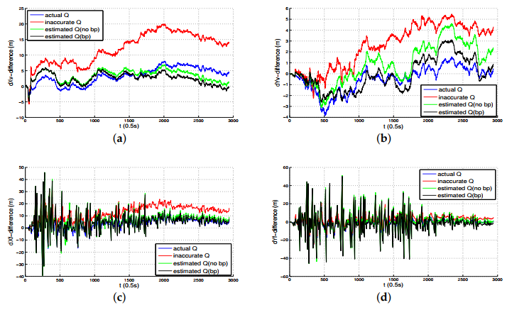
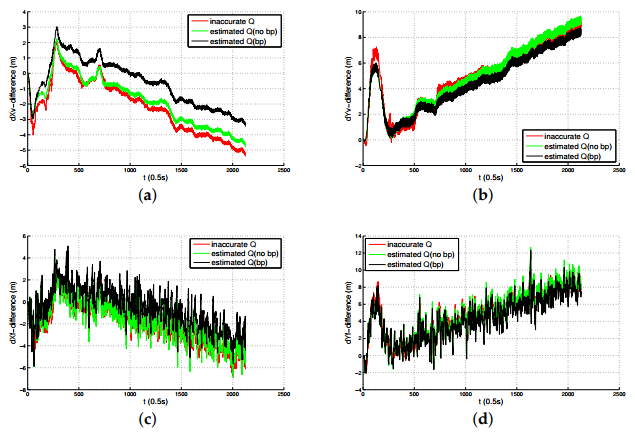
Figure 7. The positioning error of AUV and MRS, in which (a) illustrates the horizontal direction of the positioning error components of AUV in global frame; (b) illustrates the vertical direction of the positioning error components of AUV in global frame; (c) illustrates the horizontal direction of the positioning error components of MRS in global frame; (d) illustrates the vertical direction of the positioning error components of MRS in global frame.

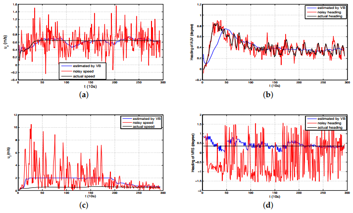
Figure 8. The forward speed and heading of AUV and MRS, in which (a) illustrates the forward speed of AUV in global frame; (b) illustrates the heading of AUV in global frame; (c) illustrates the forward speed of MRS in global frame; (d) illustrates the heading of MRS in global frame.

Table 2. The losses of proposed algorithm.

	Actual Q	Inaccurate Q	Estimated Q (without bp)	Estimated Q (with bp)
$L1$	5.6855 × 10${}^4$	5.3567 × 10${}^5$	5.7135 × 10${}^4$	3.3989 × 10${}^4$
$L2$	2.0301 × 10${}^5$	7.2603 × 10${}^5$	5.1868 × 10${}^5$	4.8194 × 10${}^5$
L	2.5986 × 10${}^5$	1.2617 × 10${}^6$	5.7582 × 10${}^5$	5.1593 × 10${}^5$

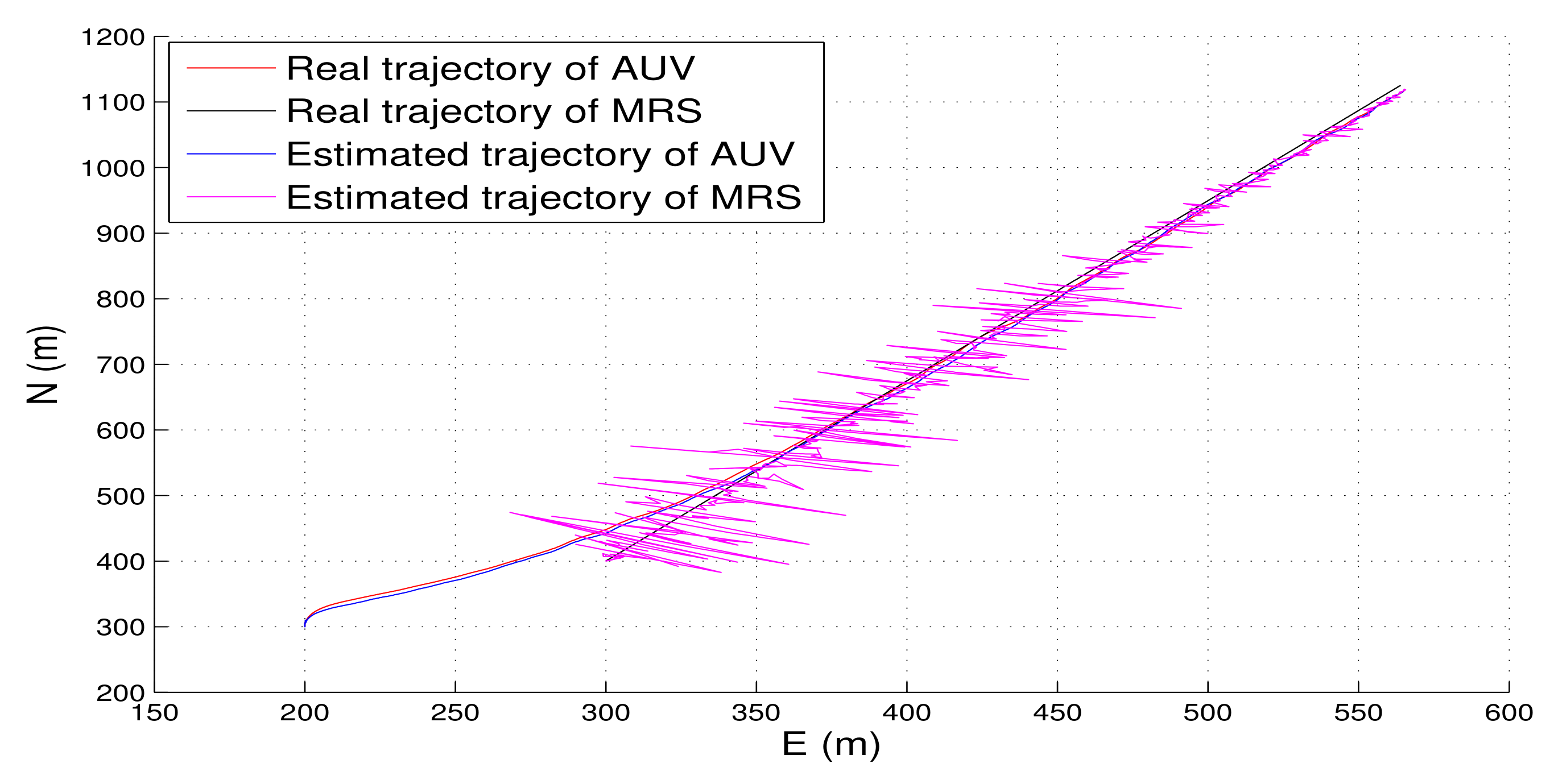
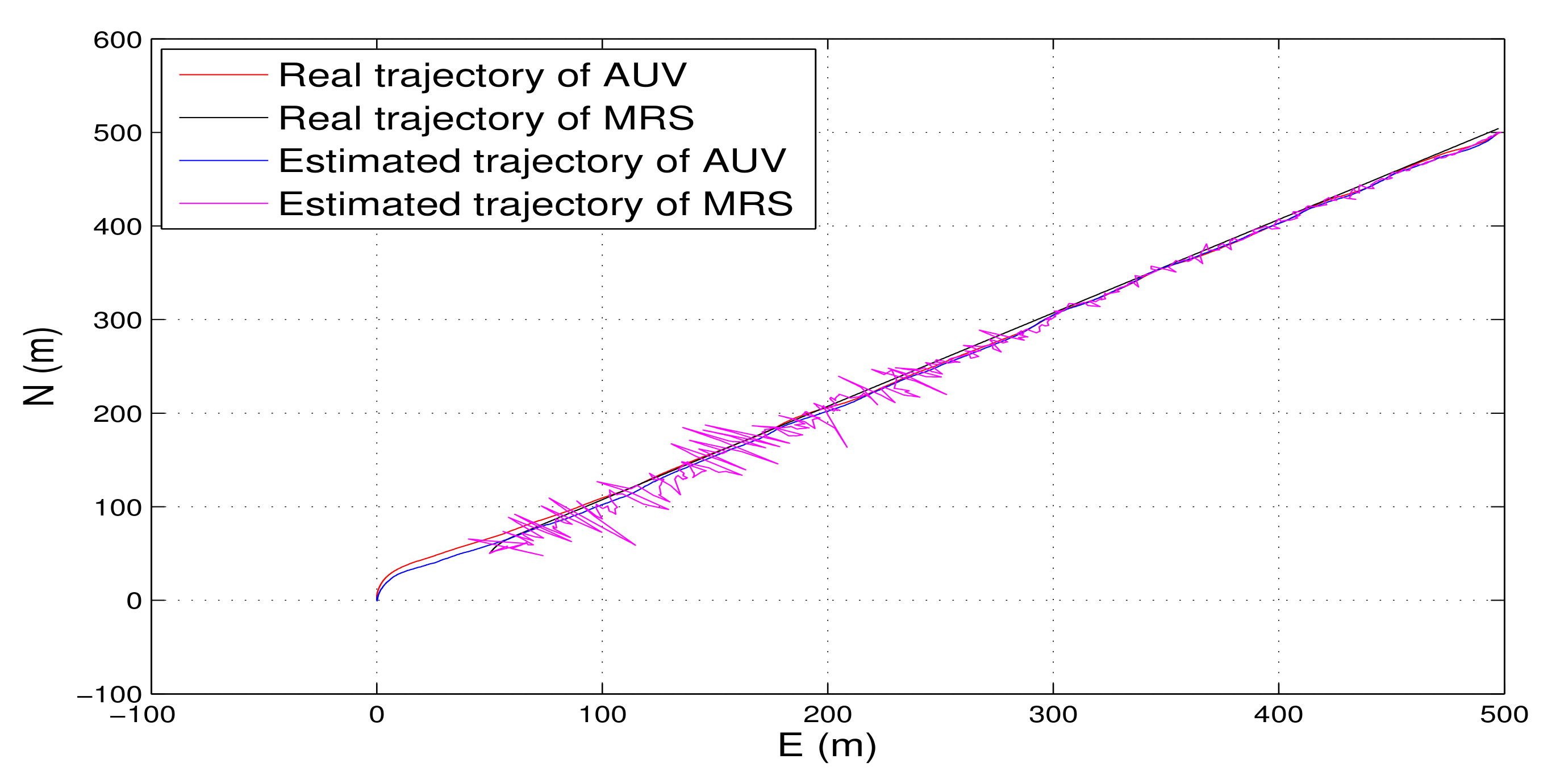
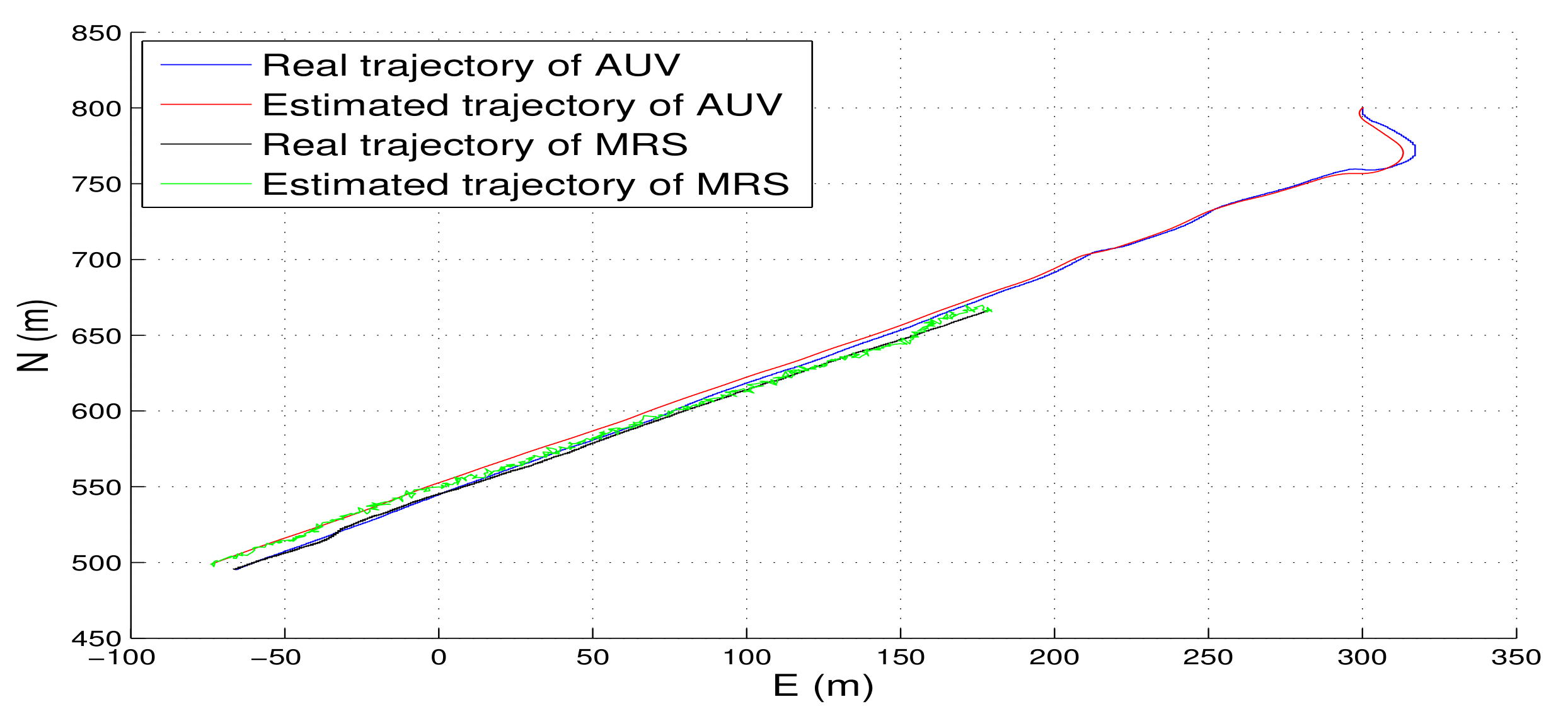
In this simulation, the real positions of AUV and MRS are calculated using the complicated motion model. The deviation between the real position and estimated position is positioning error. (a) and (b) in Figure 7 are the horizontal and vertical direction of the positioning error components of AUV with different algorithm. (c) and (d) in Figure 7 are the horizontal and vertical direction of the positioning error components of MRS with different algorithm. In these figures, the blue line show the positioning error of the TT-EKF with the PNCM ${\mathit{Q}}_2$. It should be pointed out that the components of ${\mathit{Q}}_2$ ($Q(1,1)$ and $Q(2,2)$) is the real noise statistics. The red lines show the positioning error of the TT-EKF with the PNCM ${\mathit{Q}}_1$. The PNCM ${\mathit{Q}}_1$ is totally inaccurate. The green lines show the positioning error of the TT-EKF with the PNCM is estimated by VB algorithm. The black lines show the positioning error of the TT-EKF with the PNCM is estimated by VB algorithm and the odometric error is compensated by BP neural network. The estimated heading and forward speed of AUV and MRS are shown in Figure 8 based on TT-EKF with the PNCM is estimated by VB algorithm and the prediction error is compensated by BP neural network. In (a) and (b), the red lines are noisy forward speed and heading of AUV, respectively; The black lines are actual forward speed and heading of AUV, respectively; The blue lines are the estimated forward speed and heading of AUV based on VB algorithm, respectively. In (c) and (d), the red lines are noisy forward speed and heading of MRS, respectively; The black lines are actual forward speed and heading of MRS, respectively; The blue lines are the estimated forward speed and heading of MRS based on VB algorithm, respectively. The Figure 9 illustrates the real trajectory of AUV and MRS and estimated trajectory based on adaptive TT-EKF. To compare the positioning performance of the algorithm under various conditions, Table 3 and Table 4 list the real position and estimated position of the AUV and MRS at some moments.

Figure 9. The real trajectory and estimated trajectory of AUV and MRS.

Table 3. The positions of AUV.

t	100 s	200 s	300 s	400 s
Actual position	(331.01,207.22)	(370.68,245.43)	(422.29,284.41)	(477.54,317.33)
actual Q	(329.11,207.87)	(369.25,246.80)	(423.31,285.92)	(479.70,317.90)
inaccurate Q	(323.96,207.45)	(363.40,245.09)	(414.81,283.07)	(473.37,315.39)
estimated Q(no bp)	(326.53,207.59)	(366.73,246.62)	(420.99,285.78)	(477.17,317.72)
estimated Q(bp)	(326.52,207.55)	(366.76,246.25)	(447.80,285.95)	(477.61,319.12)
t	500 s	600 s	700 s	800 s
Actual position	(535.55,344.73)	(594.86,369.41)	(654.22,393.33)	(713.85,415.49)
actual Q	(533.87,344.7846)	(592.64,368.40)	(651.53,393.00)	(712.38,416.18)
inaccurate Q	(526.65,342.11)	(584.92,365.57)	(642.26,389.63)	(700.71,412.20)
estimated Q(no bp)	(531.37,344.63)	(590.19,368.26)	(649.19,392.91)	(710.20,416.11)
estimated Q(bp)	(531.69,346.76)	(591.02,370.20)	(650.15,394.58)	(711.33,417.79)
t	900 s	1000 s	1100 s	1200 s
Actual position	(773.11,439.49)	(833.72,461.50)	(893.95,484.39)	(955.16,505.29)
actual Q	(771.08,437.31)	(829.35,458.91)	(890.63,480.38)	(953.20,502.14)
inaccurate Q	(757.83,432.76)	(817.41,454.64)	(879.46,476.35)	(942.66,498.38)
estimated Q(no bp)	(768.99,437.29)	(827.15,458.86)	(888.36,480.31)	(950.90,502.07)
estimated Q(bp)	(770.10,439.21)	(828.71,460.69)	(890.19,482.29)	(952.53,504.23)
t	1300 s	1400 s	1470 s
Actual position	(1015.0,527.84)	(1075.1,548.96)	(1116.2,564.99)
actual Q	(1015.4,525.38)	(1075.8,547.80)	(1117.3,562.70)
inaccurate Q	(1005.5,521.75)	(1066.0,544.10)	(1107.5,558.91)
estimated Q(no bp)	(1013.0,525.27)	(1073.4,547.68)	(1114.9,562.59)
estimated Q(bp)	(1014.7,527.47)	(1075.0,550.01)	(1116.6,564.98)

Table 4. The positions of MRS.

t	100s	200 s	300 s	400 s
Actual position	(425.62,309.33)	(468.55,324.95)	(518.72,343.21)	(569.95,361.86)
actual Q	(423.40,307.87)	(465.77,327.89)	(522.56,339.75)	(565.80,370.07)
inaccurate Q	(418.16,307.41)	(459.91,325.95)	(514.08,337.08)	(559.67,367.68)
estimated Q(no bp)	(420.67,307.57)	(465.98,324.37)	(519.27,342.07)	(564.27,369.43)
estimated Q(bp)	(420.66,307.53)	(466.01,324.01)	(519.80,342.23)	(564.70,370.83)
t	500 s	600 s	700 s	800 s
Actual position	(619.21,379.78)	(667.99,397.54)	(716.69,415.27)	(774.61,436.35)
actual Q	(617.92,379.42)	(664.96,395.76)	(712.44,416.51)	(772.05,436.80)
inaccurate Q	(611.10,376.80)	(657.22,392.95)	(702.91,413.09)	(760.39,432.78)
estimated Q(no bp)	(615.34,381.67)	(662.36,396.33)	(709.57,416.38)	(770.31,435.70)
estimated Q(bp)	(615.66,383.80)	(663.20,398.27)	(710.53,418.05)	(771.45,437.38)
t	900 s	1000 s	1100 s	1200 s
Actual position	(833.52,457.79)	(889.72,478.24)	(942.95,497.62)	(993.39,515.98)
actual Q	(829.13,457.78)	(880.61,481.03)	(936.05,494.27)	(986.33,516.49)
inaccurate Q	(815.99,453.40)	(868.64,476.87)	(924.83,490.16)	(975.98,512.76)
estimated Q(no bp)	(827.45,458.12)	(877.66,483.40)	(934.00,492.94)	(984.60,516.06)
estimated Q(bp)	(828.57,460.04)	(879.21,485.23)	(935.84,494.92)	(986.23,518.22)
t	1300 s	1400 s	1470 s
Actual position	(1042.4,533.81)	(1091.1,551.54)	(1125.2,563.94)
actual Q	(1037.5,533.98)	(1087.7,552.10)	(1118.7,562.71)
inaccurate Q	(1027.3,530.24)	(1077.9,548.28)	(1108.8,558.88)
estimated Q(no bp)	(1034.5,533.93)	(1085.3,551.78)	(1116.0,562.42)
estimated Q(bp)	(1036.1,536.12)	(1086.8,554.10)	(1117.7,564.81)

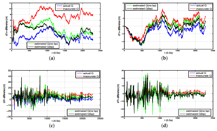
We use another set of simulation experiments to further illustrate the performance of the algorithm. The initial speed of MRS is $u_{f,0}=0.3$ m/s, the initial heading of MRS is ${\psi }_{f,0}={20}^{\circ }$ in $O_1$ coordinate frame. The initial position of MRS is $\left(x_{f,0},y_{f,0}\right)=\left(50,50\right)$. The task of MRS is to move with $u_f=0.3$ m/s and travels in a straight path with ${\psi }_f={45}^{\circ }$. The initial speed of AUV is $u_{v,0}=0$ m/s, the initial heading of MRS is ${\psi }_{v,0}=0^{\circ }$ in $O_1$ coordinate frame. The initial position of AUV is $\left(x_{v,0},y_{v,0}\right)=\left(0,0\right)$. The task of AUV is to homing to the MRS with $u_v=0.6$ m/s. The noise variance of the AUV heading is $0.01$. The noise variance of the forward speed of AUV is GMD, which contains two single Gaussian distributions. The parameters of GMD are the weights(w), mean ($\mu$) and variance ($\mathsf{\Sigma }$), which are shown in Table 5:

Table 5. The parameters of GMD.

	Weight	Mean	Variance
1	$w_1=0.6$	${\mu }_1=0$	${\mathsf{\Sigma }}_1={0.2}^2$
2	$w_2=0.4$	${\mu }_2=0$	${\mathsf{\Sigma }}_2={0.4}^2$

The PNCM $\mathit{Q}$ is initilized as $\mathit{Q}1=\left[\begin{array}{cccc}{1}^2& 0& 0& 0\\ 0& {0.52}^2& 0& 0\\ 0& 0& {0.2}^2& 0\\ 0& 0& 0& {0.07}^2\end{array}\right]$ or $\mathit{Q}2=\left[\begin{array}{cccc}{0.3}^2& 0& 0& 0\\ 0& {0.1}^2& 0& 0\\ 0& 0& {0.2}^2& 0\\ 0& 0& 0& {0.07}^2\end{array}\right]$. The simulation results are shown in Figure 10 and Figure 11.

Figure 10. The positioning error of AUV and MRS, in which (a) illustrates the horizontal direction of the positioning error components of AUV in global frame; (b) illustrates the vertical direction of the positioning error components of AUV in global frame; (c) illustrates the horizontal direction of the positioning error components of MRS in global frame; (d) illustrates the vertical direction of the positioning error components of MRS in global frame.

Figure 11. The real trajectory and estimated trajectory of AUV and MRS.

8.2. Experimental Data Analysis

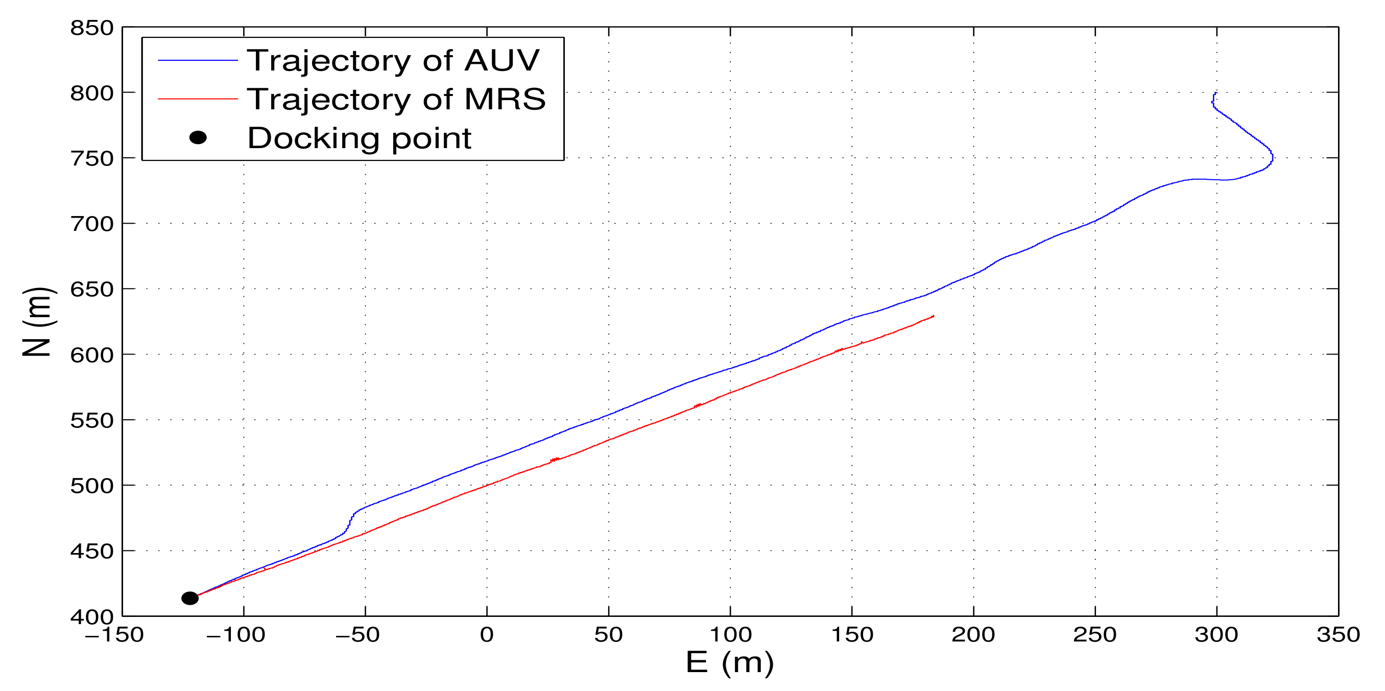
The experimental data came from the tests on a lake at the xinanjiang experimental field of the institute of acoustics, Chinese Academy of Sciences in December 2018. AUV-$II$ sensed the position of MRS by using the ultra short baseline (USBL) system. The detailed descriptions of the docking test are given in reference [24]. The Experimental results are shown in Figure 12.

Figure 12. Trajectories of AUV-$II$ and MRS recorded by IMU in AUV-$II$ homing to MRS.

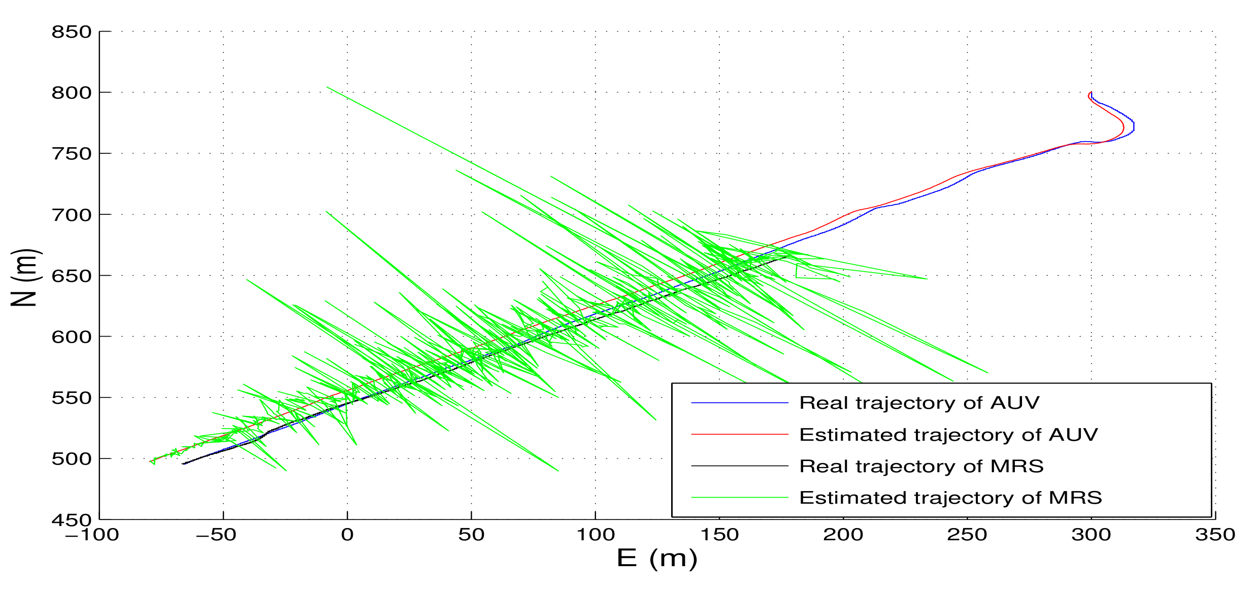
The actual PNCM of AUV-$II$ is unknown, and the PNCM is given based on experience. We compare the performance of TT-EKF algorithm and adaptive TT-EKF algorithm with this PNCM. The original Experimental data analysis results are shown in Figure 13 and Figure 14. Due to the sensor precision of AUV and the lake experimental environment, the measurement noise of AUV forward speed and heading is small. We add the same noise as the simulation to the input vector of AUV-II. The experimental data analysis results are shown in Figure 15 and Figure 16.

Figure 13. The positioning error of AUV and MRS, in which (a) illustrates the horizontal direction of the positioning error components of AUV in global frame; (b) illustrates the vertical direction of the positioning error components of AUV in global frame; (c) illustrates the horizontal direction of the positioning error components of MRS in global frame; (d) illustrates the vertical direction of the positioning error components of MRS in global frame.

Figure 14. Trajectories of AUV-$II$ and Mobile docking station(M-DS) recorded by IMU in AUV-$II$ homing to MRS.

Figure 15. The positioning error of AUV and MRS, in which (a) illustrates the horizontal direction of the positioning error components of AUV in global frame; (b) illustrates the vertical direction of the positioning error components of AUV in global frame; (c) illustrates the horizontal direction of the positioning error components of MRS in global frame; (d) illustrates the vertical direction of the positioning error components of MRS in global frame.

Figure 16. Trajectories of AUV-$II$ and Mobile docking station(M-DS) recorded by IMU in AUV-$II$ homing to MRS.

The representation of each color line in Figure 13, Figure 14, Figure 15 and Figure 16 is the same as the simulation. From the MATLAB simulation results and Experimental data analysis results, we can know that:

• As the PNCM is unknown, we assumed the PNCM is ${\mathit{Q}}_1$, which is inaccurate. The contrast between the red lines and the blue lines indicates that the inaccurate process noise statistics leads to the degradation of the state estimation performance of TT-EKF.
• The contrast between the red lines and the green lines indicates that the state estimation performance of TT-EKF has been improved with the PNCM is estimated by VB algorithm.
• The contrast between the green lines and the black lines indicates that the state estimation performance of TT-EKF has been further improved with the prediction error compensator based on neural network.

9. Conclusions

In this paper, we propose an adaptive target tracking method based on EKF with unknown non-Gaussian process noise. We use the Gaussian mixture distribution to model the noisy forward speed of AUV and MRS. We use a von Mises distribution to model the noisy heading of AUV and MRS. The parameters of these distribution are calculated based on variational Bayesian algorithm. The process noise covariance matrix is estimated according to the parameters of GMD and vM distribution. The prediction error caused by the process noise is compensated online based on BP neural network. According to the MATLAB simulation results and experimental data analysis results, we find that the state estimation performance of TT-EKF algorithm is affected by the accuracy of PNCM. If the PNCM is unknown or inaccurate, the state estimation performance of TT-EKF could be improved with the PNCM is estimated by VB algorithm. There are deviations between the real PNCM and the estimated PNCM, as well as between the real input vector and the estimated input vector. These factors cause prediction errors. The state estimation performance of TT-EKF could be further improved with the prediction error compensator based on neural network. However, the positioning error of MRS in the initial period is very large, because there is little understanding of MRS in this period. With the continuous measurement of MRS by AUV, the positioning performance of MRS is getting better and better. The future work plan includes: (1) reducing the positioning error of MRS in initial period by improving the TT-EKF algorithm; (2) the working effect of the prediction error compensator is not very satisfactory, and then further improving the performance of the neural network compensator; (3) the algorithm is tested in the ocean.

References

- Wang, Y.; Liu, K.; Feng, X. Optimal AUV trajectories for bearings-only tracking. Robot 2014, 36, 179–184. [Google Scholar] [CrossRef]
- Miller, A.B.; Miller, B. Underwater target tracking using bearing-only measurements. J. Commun. Technol. Electr. 2018, 63, 643–649. [Google Scholar] [CrossRef]
- Modalavalasa, N.; Rao, G.S.; Prasad, K.S.; Laveti, G.; Kumar, M.N.V.S.S. A new method of target tracking by EKF using bearing and elevation measurements for underwater environment. Robot. Auton. Syst. 2015, 74, 221–228. [Google Scholar] [CrossRef]
- Elhaki, O.; Shojaei, K. Neural network-based target tracking control of underactuated autonomous underwater vehicles with a prescribed performance. Ocean Eng. 2018, 167, 239–256. [Google Scholar] [CrossRef]
- Huang, Y.; Liang, W.; Yu, H.B.; Xiao, Y. Target tracking based on a distributed particle filter in underwater sensor networks. Wirel. Commun. Mob. Comput. 2008, 8, 1023–1033. [Google Scholar] [CrossRef]
- Ge, Q.; Shao, T.; Duan, Z.; Wen, C. Performance analysis of the kalman filter with mismatched noise covariance. IEEE Trans. Autom. Control 2016, 61, 4014–4019. [Google Scholar] [CrossRef]
- Durovic, Z.M.; Kovacevic, B.D. Robust estimation with unknown noise statistics. IEEE Trans. Autom. Control 1999, 44, 1292–1296. [Google Scholar] [CrossRef]
- Dong, Z.; You, Z. Finite-horizon robust kalman filtering for uncertain discrite time-varying systems with uncertain-covariance white noises. IEEE Signal Process. Lett. 2006, 13, 493–496. [Google Scholar] [CrossRef]
- Mohamed, A.H.; Schwarz, K.P. Adaptive kalman filtering for INS/GPS. J. Geol. 1999, 73, 193–203. [Google Scholar] [CrossRef]
- Odelson, B.J.; Rajamani, M.R.; Rawlings, J.B. A new autocovariance least-squares method for estimating noise covariance. Automatica 2006, 42, 303–308. [Google Scholar] [CrossRef]
- Mehra, R.K. On the identification of variances and adaptive kalman filtering. IEEE Trans. Autom. Control 1970, 15, 175–184. [Google Scholar] [CrossRef]
- Myers, K.A.; Tapley, B.D. Adaptive sequential estimation with unknown noise statistics. IEEE Trans. Autom. Control 1976, 21, 520–523. [Google Scholar] [CrossRef]
- Huang, Y.; Zhang, Y.; Wu, Z.; Li, N.; Chambers, J. A novel adaptive kalman filter with inaccurate process and measurement noise covariance matrices. IEEE Trans. Autom. Control 2018, 63, 594–601. [Google Scholar] [CrossRef]
- Sarkka, S.; Nummenmaa, A. Recursive noise adaptive kalman filtering by variational Bayesian approximations. IEEE Trans. Autom. Control 2009, 54, 596–600. [Google Scholar] [CrossRef]
- Assa, A.; Plataniotions, K.N. Adaptive kalman filtering by covariance sampling. IEEE Signal Process. Lett. 2017, 24, 1288–1292. [Google Scholar] [CrossRef]
- Gao, X.; You, D.; Katayama, S. Seam tracking monitoring based on adaptive kalman filter embedded elman neural network during high-power filber laser welding. IEEE Trans. Ind. Electr. 2011, 59, 4315–4325. [Google Scholar] [CrossRef]
- Bishop, C.M. Pattern Recognition and Machine Learning; Springer: New York, NY, USA, 2006. [Google Scholar] [CrossRef]
- Tzikas, D.G.; Likas, C.L.; Galatsanos, N.P. The variational approximation for bayesian inference. IEEE Signal Process. Mag. 2008, 25, 131–146. [Google Scholar] [CrossRef]
- Blei, D.M.; Kucukelbir, A.; Mcauliffe, J.D. Variational inference: a review for statisticians. J. Am. Stat. Assoc. 2017, 112, 859–877. [Google Scholar] [CrossRef]
- Agamennoni, G.; Nieto, J.I.; Nebot, E.M. Approximate inference in state-space models with heavy-tailed noise. IEEE Trans. Signal Process. 2012, 60, 5024–5037. [Google Scholar] [CrossRef]
- Wang, J.; Wang, J.; Shao, D.Z.X.; Chen, G. Kalman filtering through the feedback adaption of prior error covariance. Signal Process. 2018, 152, 47–53. [Google Scholar] [CrossRef]
- Wang, H.R.; Deng, Z.H.; Feng, B.; Ma, H.B.; Xia, Y.Q. An adaptive Kalman filter estimating process noise covariance. Neurocomputing 2017, 223, 12–17. [Google Scholar] [CrossRef]
- Hong, X.; Duan, K.Q.; Yuan, H.D.; Xie, W.C.; Wang, Y.L. Black box variational inference to adaptive kalman filter with unknown process noise covariance matrix. Signal Process. 2020, 169, 107413. [Google Scholar] [CrossRef]
- Zheng, R.; Lv, H.Q.; Yu, C.; Han, X.J.; Li, M.Z.; Wei, A.B. Technical Research, System Design and Implementation of Docking between AUV and Autonomous Mobile Dock Station. Robot 2019, 1–9. [Google Scholar] [CrossRef]
- Li, Q.L.; Song, Y.; Hou, Z.G. Neural network based FastSLAM for autonomous robots in unknown environments. Neurocomputing 2015, 165, 99–110. [Google Scholar] [CrossRef]
- Taghia, J.; Ma, Z.Y.; Leijon, A. Bayesian estimation of the von-Mises fisher mixture model with variational inference. IEEE Trans. Pattern Anal. Mach. Intell. 2014, 36, 1701–1715. [Google Scholar] [CrossRef] [PubMed]
© 2020 by the authors. Licensee MDPI, Basel, Switzerland. This article is an open access article distributed under the terms and conditions of the Creative Commons Attribution (CC BY) license (http://creativecommons.org/licenses/by/4.0/).