Accurate and Rigorous Calibration of Intradyne Coherent Receiver Using Polarization-Multiplexed Signal Generated within Intradyne Coherent Transmitter

Abstract

Coherent optical transceivers offer significant advantages over direct-detect optical transceivers. However, both intradyne coherent transmitters (ICT) and intradyne coherent receivers (ICR) are more complicated and require careful calibration. Traditionally, an ICR is calibrated through heterodyne beating using a single-polarized signal. Active stabilization to maintain a constant state of polarization for the calibration signal is necessary, leading to a relatively complicated setup. We demonstrate a novel method through heterodyne beating using a polarization-multiplexed signal. No polarization control is needed, resulting in a much simpler configuration. The calibration results obtained through the polarization-multiplexed signal match with the results using a single polarized signal. Moreover, this polarization-multiplexed signal can be generated within the intradyne coherent transmitter without using any external components. This innovative technique enables the calibration of a coherent receiver for deployment in the field throughout its lifetime.

1. Introduction

In contrast to the previous generation of optical transceivers relying on direct detection [1,2,3], the current generation of optical transceivers utilizes coherent detection. Coherent detection allows for the full recovery of the electrical field, including both amplitude and phase. This property allows many linear impairments, like chromatic dispersion (CD), polarization modal dispersion (PMD) and polarization dependent loss (PDL), to be compensated through digital signal processing (DSP) [4,5]. The coherent transmission exploits many degrees of freedom of photons, such as phase, polarization, amplitude, and wavelength. The state-of-the-art coherent transmitter modulates information on two orthogonal phase domains: in-phase (I) and quadrature (Q). Two orthogonal polarization domains, X and Y, are also utilized to carry the information. Thus, four tributary channels (XI, XQ, YI, and YQ) can carry modulated data. High-order modulation format, like quadrature amplitude modulation (QAM), further boosts the total capability of the coherent transceiver [6,7,8,9,10]. With so many advantages, the arrival of a coherent optical transceiver could revolutionize the optical communication industry. The history of the optical communication system could be split into two eras: before coherent detection (BC) and after direct detection (AD) [11,12].

Inevitably, the advantage and convenience provided by a coherent transceiver are accompanied by many complicated and delicate components. Here, intradyne coherent transmitters (ICT) and intradyne coherent receivers (ICR) are two essential components of the coherent transceiver. Both are much more elaborate than their counterparts used in direct detection. They require many intricate and sophisticated calibration procedures. Many parameters of the ICR must be carefully calibrated to minimize any impairment. In this paper, our focus is to reduce the complexity for this calibration. Conventionally, this calibration is performed through heterodyne beating between the internal local oscillator (LO) and the external signal generated from a tunable laser source (TLS) [13,14].

The external signal, being coherent, has a single state of polarization (SoP). To ensure that an equal amount of optical power is injected into both X polarization and Y polarization, the SoP of the TLS signal should be aligned either at 45 or 135 degrees, with respect to the principal axes of the polarization beam splitter (PBS) within the ICR. In general, a single mode fiber (SMF) is used at the input port of the ICR since both polarizations are carrying data. It is well known that SoP cannot be maintained by SMF. Thus, a critical step in this calibration is to maintain and stabilize the SoP of TLS through SMF, which requires an active control loop. However, active polarization control leads to a very complicated setup.

In addition, this method is also not suitable for calibrating the coherent transceiver in field operations. Over the lifetime of coherent transceivers and under different environments (temperature, elevation, humidity, etc.), the critical parameters of ICRs can change. It would be beneficial to perform periodic calibration of the ICR to improve the performance of coherent optical communication system. The need for an external TLS and the requirement for active SoP control prevent the in-field calibration of ICRs from being realized.

In this paper, we develop an innovative method to address the problems aforementioned. To reduce the complexity of the setup, we propose to calibrate the ICR using a polarization-multiplexed signal. Precise and complicated control of the SoP is not required in this setup, leading to a significant reduction in complexity. Furthermore, we show that the internal components of the ICT can be used to generate the polarization-multiplexed signal. One can connect the ICT to the ICR using an optical cable and perform the calibration of the ICR. The calibration of the coherent transceiver is achieved without any external components.

The article is organized as follows: In Section 2, we discuss how the ICR is traditionally calibrated using a single-polarization laser source. We also show the influence of the operation mode of the trans-impedance amplifier (TIA) within the ICR. In Section 3, we demonstrate the formation of a polarization-multiplexed signal using two external lasers. The calibration results using the polarization-multiplexed signal agree well with those obtained with the traditional method. In Section 4, we demonstrate the generation of the polarization-multiplexed signal using the internal components of the ICT. Furthermore, we show our detailed steps and the calibration results. In Section 5, we draw our conclusions.

2. Traditional Calibration Method of Intradyne Coherent Receiver Using Single-Polarized Signal

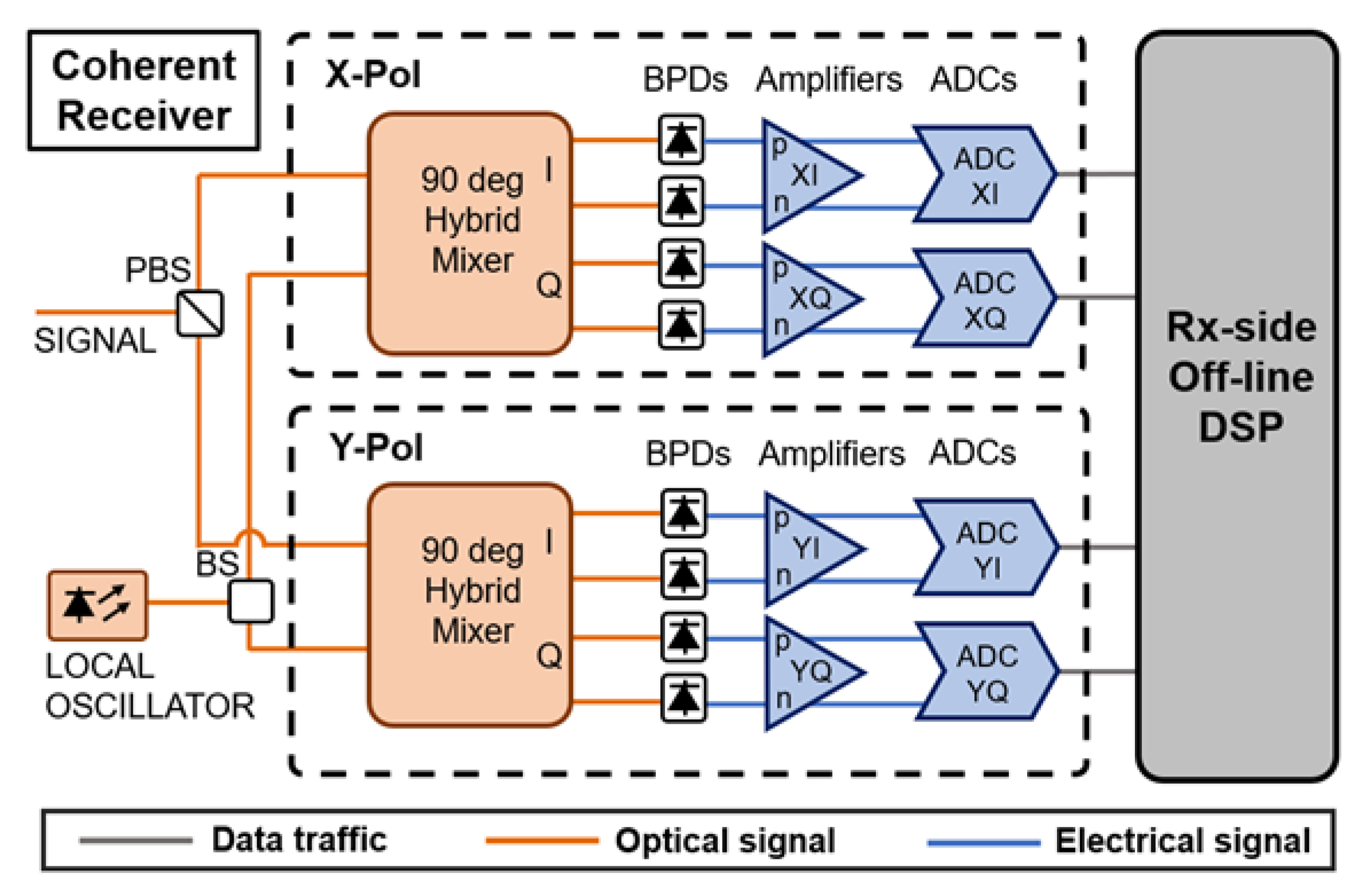
The ICR can be divided into two parts: an analog front end and a digital back end. The analog front end of ICR is composed by a PBS, a 90-degree optical hybrid, four pairs of balanced photo diodes, and four sets of TIAs. The digital back end of the ICR is composed by analog digital converters (ADC) and a DSP application-specific integrated circuit (ASIC). The interface between the analog front end and digital back end may include high-speed radiofrequency (RF) traces or RF connectors. A block diagram of ICR is shown in Figure 1.

Frequency response, bandwidth, skew, gain imbalance, and quadrature angle are the critical parameters of analog front end of the ICR. Smooth frequency responses without abrupt changes for all tributaries are desired. The bandwidth of the ICR should be sufficient, otherwise a significant penalty in the required optical signal-to-noise ratio (OSNR) is introduced. The bit error rate (BER) will suffer if the skew among different tributaries of the ICR is large. The impact is even more severe for the skew between the I tributary and Q tributary [15]. Distortion in the constellation diagram is introduced when the gain imbalances among different tributaries are not compensated, leading to reduced system performance. The ideal quadrature angle should be 90 degrees. Any deviation from ideal value leads to the crosstalk between the in-phase signal and the quadrature signal. Those parameters discussed above should be carefully measured during the initial calibration. Once characterized, many impairments due to non-ideal parameters can be compensated through DSP [16,17,18,19,20,21,22].

Many critical parameters of the ICR can be calibrated through the exploitation of the heterodyne beating between two continuous-wave (CW) signals. One signal is from the internal LO within the ICR. The other signal is generated from an external TLS. The heterodyne beating creates a sinusoidal signal at the outputs of TIAs, whose frequency is the frequency difference between TLS and LO. By sweeping the frequency of the TLS and maintaining the frequency of the LO, the frequency of the sinusoidal beating signal is continuously varied. During this process, both TLS and LO should maintain a constant output power. In this way, frequency sweeping in the baseband of ICR can be performed, and many critical parameters of ICR can be derived from this frequency sweeping. The curve of amplitude versus frequency determines the frequency response and the signal bandwidth. The difference in amplitude response among four tributary channels corresponds to the gain imbalance. The phase difference between the I tributary and Q tributary is used to calculate the quadrature angle. The skew can be derived by examining the curve of phase versus frequency.

One important, yet subtle, aspect during the calibration of coherent ICR is to set the appropriate operational mode of TIA within the ICR. In the normal operation, the TIAs should be in the automatic gain control (AGC) mode to ensure that the electrical outputs of TIAs remain constant even when there is any change or transient of receiving optical power. It is natural to assume that the TIAs should be in AGC mode during the calibration of ICR. However, there is a big difference in the characteristics of the input signal to the ICR. During normal operation, the input signal is broadband with multiple frequencies. The AGC mode is used to compensate the change in the optical power, while the gain across the whole spectrum remains constant. In a stark contrast, the input signal contains a single frequency during the calibration through heterodyne beating. When the frequency difference between TLS and LO is large, the outputs from the TIAs will be reduced due to the limited bandwidth. If one sets the TIA to AGC mode, the gain in TIAs will be adjusted to compensate the limited bandwidth. However, this is not the intended usage of the AGC mode. Thus, it is critical to set the TIA to manual gain control mode (MGC). This will ensure that the gain of the TIAs remains constant during the frequency sweeping. In certain aspects, the MGC mode in the heterodyne measurement resembles the AGC mode in normal operation mode.

The performance of a standalone individual ICR is measured using the heterodyne beating method described above. The outputs of TIAs are sampled and post-processed by an optical modulation analyzer (OMA, Keysight N4392, Santa Rosa, CA, USA). The results in both the MGC mode and the AGC mode are shown in Figure 2. In the MGC mode, the gain of the TIAs remains constant during the calibration. The peaks in the frequency response are located at approximately 17.5 GHz. To determine a 3-dB bandwidth, we measure the response at 0.5 GHz. Then, we find the frequency where the response is 3 dB lower than that at 0.5 GHz. The YI and YQ tributaries have a 3-dB bandwidth of approximately 25 GHz, and the XI and XQ tributaries have a 3-dB bandwidth of approximately 26 GHz. In the AGC mode, the gains of the TIAs are adjusted to maintain constant peak–peak swing at outputs of TIAs for different frequencies. An ‘artificial’ flat frequency response from 5 GHz to 17.5 GHz is observed. However, a real broadband signal with multiple frequencies will not experience this frequency response. One can also notice that any intrinsic gain imbalance among different tributaries is removed in the AGC mode. It is important to operate TIA in the MGC mode during the calibration, which represents the real application scenario.

As discussed in the introduction, a critical step is to control the SoP of TLS launching into the ICR. Ideally, the SoP of TLS should be aligned at either 45 or 135 degrees with respect to the principal axes of the PBS in the ICR. This will guarantee that equal amounts of optical power are sent to both the X polarization and Y polarization. An active control loop for SoP, formed by an automatic polarization controller and a polarimeter, is needed to maintain the SoP at the input port of ICR. Figure 3 shows the typical configuration using the heterodyne beating method. Because SMF is used to connect the output of polarization control to the input of ICR, one needs to add a manually adjustable polarization controller in between. This is to ensure that the SoP at the input to the ICR is the same as the SoP at the input of the polarimeter.

The typical steps to set up the polarization controller are as follows: first, one sets the automatic polarization controller so that the SoP to the polarimeter is linearly polarized along one polarization (for example, X polarization). We use a Keysight N7788 (Santa Rosa, CA, USA) component analyzer, which contains both the automatic polarization controller and the polarimeter. Next, one adjusts the manual polarization controller so that the outputs of TIAs from the other polarizations (for example, Y polarization) are minimal. This will ensure that the inputs to both polarimeters and the ICR have the same SoP. Finally, one sets the automatic polarization controller so that the SoP is linearly polarized at 45 degrees or 135 degrees. The automatic polarization controller will maintain a constant SoP based on the internal feedback from the polarimeter.

Figure 4 shows the results obtained with OMA N4392 with active stabilization turned on. In the subfigure (a), the frequency difference between the TLS and the LO is 2.5 GHz, showing the response of the ICR near the direct current (DC) frequency. In the subfigure (b), the frequency difference between the TLS and the LO is 22.5 GHz, showing the response of the ICR at a high frequency. There are six traces: traces A and B are the spectral responses of X polarization and Y polarization; traces C to F are the time domain signals for four tributary channels. The frequency difference can be clearly identified by the locations of peaks in traces A and B. The peak-to-peak swing of traces C to F reduces when the frequency difference is swept from 2.5 GHz to 22.5 GHz, demonstrating the impact of bandwidth on the output of ICR. The difference in the time domain signal within the same polarization (XI vs. XQ, or YI vs. YQ) is caused by the IQ imbalance between the I tributary and Q tributary. Most importantly, the XY imbalance, defined as (XI + XQ)/(YI + YQ), remains very small when the frequency is swept from 2.5 GHz to 22.5 GHz. This shows that the active stabilization maintains an ideal SoP. Thus, both polarizations are injected with an equal amount of power.

To further manifest the necessity of the active stabilization of the SoP, we measure the response of ADC when the active stabilization of the SoP is not engaged. In addition, we demonstrate that ICR calibration can be performed within the coherent transceiver. Instead of using an OMA to analyze the signal, we measure the electrical output of the ICR integrated within a pluggable CFP2 form-factor pluggable analog coherent optics module (CFP2-ACO), as specified by Optical Internetworking Forum (OIF) [23]. Here, the pluggable module is a class-2 CFP2-ACO with a linear RF amplifier, which can support a 200 Gb/s (gigabit per second) data rate using the DP-16QAM modulation format at a baud rate of approximately 30 GBd. The detailed characteristics of this CFP2-ACO module can be found in [24]. The outputs of ICR are sampled by DSP ASIC in the receiver side and stored in the internal memory. We download the waveforms from the memory and perform post-processing. We measure the output of the ICR four times without using active SoP stabilization. Next, we plot the output of the I tributary along the X axis and plot the output of the Q tributary along the Y axis, forming the typical Lissajous curves. As shown in Figure 5, the Lissajous curves change dramatically when the SoP of the input signal drifts around. An active stabilization of the SoP is indeed needed for the accurate calibration of ICR using the traditional method.

3. Innovative Calibration of Intradyne Coherent Receiver Using Polarization-Multiplexed Signal

We propose a simple yet elegant solution to resolve the issue discussed in Section 2. The solution is to use a polarization-multiplexed signal to perform the heterodyne calibration of the ICR. The polarization-multiplexed signal contains two orthogonal polarization components with equal power. Even if one intentionally introduces some random polarization rotation in the SMF, an equal amount of power will always be projected into both X and Y polarizations. Thus, there is no need for the active stabilization of SoP, which greatly reduces the complexity of the calibration setup. Note that one needs to make sure that the two polarization components are not coherent with each other. Otherwise, a light with elliptical SoP will be generated. Its SoP cannot be maintained by the SMF. The degree of polarization (DoP) is the important characteristic in this case. For the polarization-multiplexed signal, the DoP should be very close to zero.

There are two ways to generate the polarization-multiplexed signal. The first way is to combine the outputs of two separate TLSs with orthogonal polarizations through a polarization beam combiner (PBC). Two TLSs should have the same frequency and output power. One should note that, although two TLSs have the same frequency, their outputs are not coherent with each other since the outputs are coming from two individual TLSs. If the two TLSs have the same SoP initially (for example, along X polarization), one can insert a polarization rotator in one path to rotate the SoP along the Y polarization. A half-wave plate whose principal axis is aligned at either 45 degrees or 135 degrees can serve as the polarization rotator. The polarization-maintaining fibers are required before the PBC. The outputs from the PBC are effectively polarization-multiplexed signals, with the DoP being close to zero, as shown in Figure 6.

To demonstrate the feasibility of this innovative method, we calibrate the same ICR integrated into the CFP2-ACO module using the polarization-multiplexed signal. We choose to form the polarization-multiplexed signal using two individual TLSs. We remove the automatic polarization controller, the polarimeter and the manual polarization controller from the setup since we do not need to precisely control the SoP anymore. No matter how the SMF changes the polarization of the signal, there will be always equal amounts of optical power projected into the X and Y polarizations. We illustrate this by showing the Lissajous curves in a few scenarios in Figure 7.

During the calibration, the frequencies of two TLSs are simultaneously tuned to create the frequency sweeping. Similarly, the outputs of ICR are sampled by DSP ASIC and stored in the internal memory. The waveforms are further downloaded and post-processed. The critical parameters of ICR are measured. As seen, the outputs of ICR experience very small changes even without any SoP control, demonstrating the advantage of using a polarization-multiplexed signal as the calibration signal.

Figure 8 shows the comparison between the results obtained using two calibration methods. One method measures the bandwidth using the single-polarization configuration with active stabilization on, while the other method measures the bandwidth using the dual-polarization method with active stabilization off. As seen, the two methods give very close results, demonstrating that one can use the polarization-multiplexed signal to calibrate the coherent ICR. We notice a small deviation between the two results. The likely root cause is the drift of SoP in the single-polarization measurement. As seen in Figure 3, an SMF connects the output of the polarization controller with the input of ICR. Since the SMF cannot maintain SoP, the drift of SoP will lead to errors in the measurement. We can eliminate this issue by using the polarization-multiplexed signal.

The second way is to use a single TLS to generate the polarization-multiplexed signal. Compared with the first way, the second way removes the requirement for two TLSs and eliminates the efforts to match the frequency and power for two TLSs. First, a beam splitter (BS) splits the output of the TLS into two paths. The polarization in one path is rotated by 90 degrees using a half-wave plate. Then, these two paths are recombined using a PBC. Polarization maintaining fiber (PMF) is required for both paths. The length difference between two paths needs to be larger than the coherence length of TLS. A wide laser linewidth leads to a short coherent length. Thus, a low-cost TLS with large linewidth is well suited for this application. Figure 9 shows this configuration. The wavelength accuracy of low-cost TLS might be low. As demonstrated later in Section 4, we can measure the frequency difference between the TLS and the LO very accurately by performing Fourier transform on the output signal of the ICR. This will address the concern of using the low-cost TLS for ICR calibration.

4. Generation of Polarization-Multiplexed Signal Using Intradyne Coherent Transmitter

The setup shown in the previous section is mostly suitable for the initial calibration of ICR in the laboratory environment or on the manufacturing floor. The reason is that the external TLSs are used to create the polarization-multiplexed signal. It is highly desirable to further simplify the setup and eliminate any usage of external components. By generating the polarization-multiplexed signal, relying only on the internal components within the ICT, one can implement the calibration of the ICR, providing significant advantages and flexibility.

To implement this, we examine the building blocks of a coherent IQ transmitter, as shown in Figure 10. It is composed of an optical front end and an electrical back end. In the electrical back end, a block of forward error correction (FEC) firstly encodes the data. Next, a finite impulse response (FIR) filter in the tap-and-delay structure compensates many impairments. Then, a high-speed digital-to-analog converter (DAC) converts the output of the FIR filter from the digital domain to the analog domain. Finally, the analog electrical signal goes through RF traces on print circuit board (PCB) and the pluggable RF connector (in some implementations). Four linear RF amplifiers boost the signal and drive the Mach–Zehnder modulators (MZM). In the optical front end, the output from a CW TLS is firstly split into four tributaries and fed into the MZMs. Next, the optical signal is modulated by MZM based on the output of the RF amplifier. Then, a phase modulator (PM) is used to introduce a 90-degree difference between the I tributary and Q tributary. On one optical path, the polarization is rotated by 90 degrees by using a polarization rotator (Pol-Rot). Finally, a PBC is used to combine the outputs from two polarizations.

As seen, all components for the generation of a polarization-multiplexed signal, using the second way described in Section 3, have been built in an ICT. However, some additional steps are required. In order to minimize the skew between polarizations, the length of optical path in the X polarization is the same as that in the Y polarization. If the modulation signal is not applied to MZM, the signals from two polarizations will be coherent with each other. The DoP of the combined output from the PBC is close to one, and the SoP of the combined output can drift and fluctuate over time. To prevent this from happening, one can apply one small frequency shift (F_x) through the MZMs in the X polarization, and another small frequency shift (F_y) through the MZMs in the Y polarization. If the absolute difference between F_x and F_y is larger than the linewidth of TLS, the signal from the X polarization will no longer be coherent with the signal from the Y polarization. Moreover, the DoP of the combined output from PBC is close to zero. In this manner, a polarization-multiplexed signal is generated from an ICT.

Two data paths exist in the DSP ASIC before the ICT. One path is the regular data traffic, which passes through the FEC block, the FIR filter and the DAC. The other path is through a built-in memory within the DSP ASIC. A user-defined data pattern can be loaded into this memory. The output of DAC will correspond to the data within the memory. Once the end of the memory is reached, the output will go back to the beginning of the memory in a round-robin way. The outputs of DAC are first amplified and then modulate the optical signal through the MZM. One can switch the data path between regular data traffic and the memory in ASIC. In this work, we load the ASIC memory with the desired data pattern to create the necessary frequency differences for the polarization-multiplexed signal.

In [25,26,27,28,29,30], a method to apply a frequency shift to the output of ICT has been demonstrated through applying particular driving signals to the MZM. Following the same methodology, we loaded the memory into the DSP ASIC as follows:

$$\begin{array}{l}XI(n)=DA{C}_{\max }\ast \cos (2\pi \ast F_x\ast n)\\ XQ(n)=DA{C}_{\max }\ast \sin (2\pi \ast F_x\ast n)\\ YI(n)=DA{C}_{\max }\ast \cos (2\pi \ast F_y\ast n)\\ YQ(n)=DA{C}_{\max }\ast \sin (2\pi \ast F_y\ast n)\end{array}$$

(1)

where DAC_max is the maximum value in the output of DAC, n is the index within the memory. For an 8-bit DAC with the most significant bit (MSB) being the sign bit, DAC_max is equal to 128. The value is rounded to the nearest integer and loaded into the memory in the two’s complement fashion.

In the ICT, the bias points of the MZMs should be at the null points. In normal operation, automatic bias-control loops (ABC) are enabled to prevent the bias points from drifting away. The ABC loops work as desired when the regular data (with a broad spectrum) path is chosen. We observed that the ABC loop could lose its tracking when the memory data path is chosen. This is due to the fact that the sinusoidal function within the memory has a narrow spectrum. To prevent this from happening, the MZM is firstly driven by regular data traffic so that the ABC loop locks the bias to the null point. Next, ABC loops are frozen so that the bias points do not change further. Finally, the data path is switched from regular data traffic to the sinusoidal wave within its memory.

Also, the ICT should use a linear RF amplifier instead of a limiting RF amplifier. The reason is that the limiting RF amplifier will distort the sinusoidal wave and create undesired high-order harmonics. Similar to TIA in the ICR, there are two operational modes for the RF amplifier: the AGC mode and MGC mode. In the normal operation using regular data, the RF amplifier should be in AGC mode to dynamically compensate any variation in the data path. In the calibration process using data in memory, the RF amplifier should be in MGC mode so that its gain remains constant when the frequency of the sinusoidal waveform changes during the process. The reason behind this is the same as the reason for the mode of the TIA, as described in Section 2.

Figure 11 shows the measured DoP versus the frequency difference between two polarizations |F_x-F_y|. As seen, the DoP keeps decreasing when |F_x-F_y| increases. When |F_x-F_y| is larger than 0.94 GHz, the DoP is very close to zero. The residual DoP is due to the power imbalance in ICT. Figure 12a shows the measured DoP and output power versus time. During this measurement, we switch from the regular data to the calibration waveform loaded in memory. After the switching, the DoP is very stable and close to zero. Figure 12b shows the spectrum measured by Keysight OMA N4392. We choose OMA to perform this measurement since the polarization-demultiplexing algorithm within OMA can separate the signal into two orthogonal polarizations. One can clearly identify the frequency shift between two polarizations. Small side lobes are noticeable in this spectrum due to the fact that only a fundamental frequency component is used to modulate the MZMs for simplicity. To eliminate those side lobes, one needs to include the high-order harmonics of fundamental frequency, which can cancel out those side lobes.

Having generated the polarization-multiplexed signal from the ICT, we further adjusted the carrier frequencies of the TLS in the ICT (defined as LO_tx) and the carrier frequency in the ICR (defined as LO_rx). This creates a frequency difference and generates a heterodyne beating signal in the outputs of the ICR. By sweeping the frequency difference (|LO_tx – LO_rx|) over the baseband of the ICR, one can determine many critical parameters. Although two frequency components are 0.94 GHz apart, the frequency response and other critical parameters of the ICR will not change drastically over this small range. Thus, we can use the average value of two frequency components, shown in the equation below, to represent the setting value of the heterodyne beating frequency.

F_set = | LO_tx − LO_rx| + (F_x + F_y)/2

(2)

In the receiver side of the DSP ASIC, the raw data from the ADC outputs is saved as a snapshot. We converted the ADC raw data from the time domain to the frequency domain through fast Fourier transform (FFT). From the results in the frequency domain, we can identify two peak frequencies in the spectrum, roughly corresponding to |LO_tx–LO_rx| + F_x and |LO_tx–LO_rx| + F_y. The tuning of the carrier frequency of the local oscillator from the pre-defined wavelength grid is implemented through the temperature control of TLS. Thus, over the lifetime of the coherent transceiver, the actual detuning could be different from the set detuning. Instead of relying on the setting value of F_set, we identify two peak frequencies within the frequency spectrum (f_peak1 and f_peak2) and determine the actual heterodyne beating frequency f_meas = (f_peak1 + f_peak2)/2. This will further improve the accuracy of calibration procedure. Figure 13 shows the two measured peak frequencies f_peak1 and f_peak2 versus the setting beating frequency F_set. Typical FFT spectrums are also shown. As seen, an accurate linear relationship exists between F_set and f_meas.

Figure 14 shows the frequency response of a coherent transceiver on the Rx side, which includes the ICR integrated in the CFP2-ACO transceiver, the RF PCB traces, the pluggable connector and the DSP ASIC. In this figure, the measured value of f_meas is plotted along the X axis. For each value of f_meas, we measure 16 times to improve the calibration accuracy. The peak-to-peak swing of ADC raw data for four tributaries (XI_swing, XQ_swing, YI_swing, YQ_swing) are first determined in the time domain. Then, their distribution is shown as a boxplot. Some fluctuations in the peak-to-peak swing are observed. The likely root cause for fluctuations is that some high-order harmonics are generated when the fundamental sinusoidal wave is loaded and played from the memory in DSP ASIC. The measurement accuracy can be further improved by loading the memory with more complicated data to remove those high-order harmonics.

The frequency response of four tributaries are determined from the median values of peak-to-peak swing. We used the median value instead of the average value. The reason is that the median value is very tolerant to any outliers in the measurements, while the average value is strongly influenced by the outlier measurements. In current setup, the maximum frequency difference between two LOs is 15 GHz, limited by how far the frequency of LO can be detuned from a pre-defined frequency grid. Our results indicate that the 3-dB bandwidth of this coherent transceiver on the Rx side is larger than 15 GHz for all tributaries. The IQ gain imbalance in X polarization is 0.29 dB. The IQ gain imbalance in Y polarization is -0.35 dB. Finally, the gain imbalance between polarizations is 0.25 dB.

IMB_IQ,X = XQ_{swing_median}/XI_{swing_median}
IMB_IQ,Y = YQ_{swing_median/}YI_{swing_median}
IMB_XY = (XQ_{swing_median} + XI_{swing_median})/(YQ_{swing_median} + YI_{swing_median})

(3)

Usually, within a coherent transceiver, the coherent receiver shares the same TLS with the coherent transmitter as the LO for the benefit of cost reduction. In the method discussed above, the heterodyne beating is generated by detuning the frequency of the coherent transmitter from the frequency of the coherent receiver through thermal control. We keep F_x and F_y to very small values to minimize any influence of the modulation bandwidth on the coherent transmitter. Thus, the calibration procedure above will require the ICR and ICT to be located in different coherent transceivers. It is achievable since there are normally multiple coherent transceivers within a host line card. One can connect the Tx output of one module to the Rx input of its neighboring module through an SMF.

Moreover, it is possible to implement the calibration procedure using the ICR and the ICT within the same coherent transceiver. As seen from Equation (2), the beating frequency contains two parts: the frequency difference between the Tx LO and the Rx LO, and the average value of F_x and F_y. If the LO is shared between Tx and Rx, the first term is zero. One can increase both F_x and F_y simultaneously to increase the heterodyne beating frequency F_set. Meanwhile, |F_x–F_y| should be kept larger than 0.94 GHz to depolarize the combined output. However, when a large frequency shift is introduced, the combined output power will be reduced due to the limited modulation bandwidth of the MZMs. Most ICTs have integrated photo diodes to monitor the output power and most ICRs have integrated photo diodes to monitor the input power. One can use those photo diodes to monitor the power of the polarization-multiplexed signal, as shown in Figure 15. The influence of the power change can be deducted from the calibration result of the ICR. In this way, the self-contained calibration of the tcoherent transceiver can be achieved by looping back between its transmitter and its receiver.

5. Conclusions

Many important parameters for ICR are measured using the heterodyne beating method. The memory within the DAC of the DSP ASIC is loaded with a sinusoidal waveform. The frequency of the sinusoidal waveform in the X polarization is different from that in the Y polarization. When the difference is more than the linewidth of a laser, a polarization-multiplexed signal is produced at the output of the ICT. The significant advantage of using polarization-multiplexed signal lies in the fact that no active SoP control is needed. An SMF cable can connect the output of ICT to the input of ICR, and one can perform the calibration of ICR using heterodyne beating.

The raw data from the ADC snapshot is analyzed. The frequency response, 3-dB bandwidth, and gain imbalance are determined. Any imperfections can be compensated in the digital domain through the FIR filter. This simple yet accurate procedure can be carried out during deployment in the field over the lifetime of a coherent transceiver.