Abstract
In this study, we introduce an adaptive model-free coupling controller while using recurrent fuzzy neural network (RFNN) for multi-axis system to minimize the contour error. The proposed method can be applied to linear or nonlinear multi-axis motion control systems following desired paths. By the concept of cross-coupling control (CCC), multi-axis system is transferred into a nonlinear time-varying system due to the time-dependent coordinate transformation; tangential, normal, and bi-normal components of desired contour. Herein, we propose a model-free adaptive coupling controller design approach for multi-axis linear motor system with uncertainty and nonlinear phenomena. RFNN establishes the corresponding adaptive coupling controller to treat the uncertain system with nonlinear phenomenon. The stability of closed-loop system is guaranteed by the Lyapunov method and the adaptation of RFNN is also obtained. Simulation results are introduced in order to illustrate the effectiveness.
1. Introduction
In industrial applications, multi-axis motion systems have been applied many machining systems, e.g., machine tools, position stage of semi-conductor equipment, and robot manipulators. The contour error is usually adopted to evaluate the control performance; it is defined as the error component orthogonal to the desired path.
For practical mechanical control systems, the contour error always exists due to mechanical structure, servo lag, as shown in Figure 1 [1,2,3], ec: contour error, ewy: tracking error in y axis, and ewx: tracking error in x axis. Obviously, the tracking error is calculated every time instant and the contour one is not by instant; therefore, reducing tracking error does not effectively reduce the contour error. However, the trend of smart manufacturing is high speed and accuracy; therefore, the minimization of contour error is more important. Recently, most of industrial controllers used are PID controllers and multi-axis synchronization is less common. The key point is to design the appropriate trajectories (CNC controller interpolation, acceleration, and deceleration planning) to achieve the purpose of precision machining. Subsequently, the multi-axis control approach as proposed to treat it [4,5,6,7,8,9,10,11,12,13,14].
Figure 1.
Calculation diagram of Contour error [1,2,3].
Literature [4,5,6] introduced the cross-coupling controller (CCC) concept to reduce the contour error. The CCC minimizes the contour error, rather than reducing the individual axis errors by the synchronization concept, and variable-gain cross-coupled controllers can instantly adjust compensator gain value based on different path models to reduce contour error, but there are restrictions on the velocity and curvature of each axis [5]. A modified variable-gain that is based on CCC scheme is proposed in [7], in which the actual contour error was replaced as a linear contour approximation to reduce the computational complexity. Recently, there are several approximated methods of contour error, and literature [8] proposed equivalent error controller design rule. The corresponding contour error model should be constructed. Literature [9,10] introduced three-dimensional contour error estimation methods, and a coordination transformation system was introduced to change the coordinates of multi-axis system to time-variable coordinates and calculate the contour error in time instant, as shown in Figure 2. Subsequently, an adaptive controller with linear regression property for a second order system was proposed [11]; however, the derivation of linear regression is complicated and difficult to obtain for system uncertainty. Literature [12] also utilized the local approximation of the desired path to propose a static contour error estimation method. On the other hand, dynamic estimation methods of contour error based on the Newton algorithm were introduced for achieving high precision [13,14,15], such approaches are typically limited by the assumptions of system dynamics should be exactly known. For a practical nonlinear plant, the system is usually not exactly known or having uncertainties or external disturbance; therefore, this motivates us to establish the adaptive model-free control method, even the controlled systems having un-modelled uncertainties and nonlinear phenomenon.
Figure 2.
Time-varying coordinate frame [11].
Linear motors have high complexity nonlinear phenomena of friction and ripple forces. To treat this problem, literature [16,17,18,19] introduced a force ripple compensation scheme based on a simple and compact model of the disturbance, and literature [20] presented three different models of friction in pre-sliding regime on linear motor platform. Herein, we propose an adaptive model-free coupling controller design while using RFNN to minimize the contour error of multi-axis linear motor system with uncertainty and nonlinear phenomenon. A time-varying contour error definition that is based on the transformation matrix is established and the design of the trajectories under the Cartesian coordinates is converted into time-varying coordinate command. The Lyapunov theory is used to guarantee the asymptotic stable of contour error and the adaption of RFNN weighting vector is also obtained.
2. Multi-Axis Systems and Recurrent Fuzzy Neural Networks
2.1. System Description
The dynamic model of a multi-axis linear motor system is
where denote the measurable position, velocity, and acceleration of system (1), respectively; and denotes the system unknown diagonal mass and viscous friction matrices; and, represents the control input; denotes the force ripple disturbance; denotes the frictional force. In this study, system mass, viscous, force ripple, and frictional force are assumed to be unknown or with uncertainties. Use the concept of [11], the multi-axis system coordinate can be transformed to contour plant by time-varying transformation F(t) = [t(t) n(t) b(t)]. According the results of [11], is composed of a unit tangent vector, ; unit normal vector, ; and, bi-normal vector, . Vectors t(t), n(t), and b(t) are calculated by the tangent and normal components of a desired trajectory xd(t). For multi-axis system, the desired trajectory is generated by computer numerical controller (CNC) interpolation of motion control. Therefore, xd(t) is differentiable of class C3 in practical used.
By the time varying transformation, we have
where , and denote the position, velocity, and acceleration of system (1) and desired path expressed in the time-varying coordinate system, respectively, as shown in Figure 2. Based on Equations (2) and (3), system (1) is transformed as
where , , , , , and ,
According the results of [11], System (4) has the following properties, being utilized to establish a regression-based adaptive approach.
- (a)
- Symmetric: mass matrix is symmetric, positive definite [11,18].
- (b)
- Skew-symmetric: matrices and skew-symmetric and satisfy , .
- (c)
- Linear parameterize: system (4) can be linearized parameterized , where contains the unknown constant system parameters and denotes a regression matrix [11].
However, practical systems usually contain un-modeled uncertainties and nonlinear phenomenon; the above properties do not hold. This results in the adaptive coupling controller of [11] not being valid. Therefore, the control objective of this paper is to establish an adaptive model-free coupling controller for multi-axis system to drive the system follows the contour. As above, we define the instant contouring error as , where and are position of system (4) and desired path expressed in the time-varying coordinate system. This means that our goal is to develop adaptive model-free controller to minimize the contouring error e. In this study, we utilize the RFNN to develop a model-free adaptive coupling controller to result in high precision and synchronization control of machine tools. In the following, a brief introduction of RFNN is given.
2.2. Recurrent Fuzzy Neural Network
In this study, we introduce an adaptive model-free coupling controller while using recurrent fuzzy neural network (RFNN) for multi-axis system with uncertainties to minimize the contour error. The architecture diagram of RFNN is shown in Figure 3 [21]. The RFNN is a generalization of fuzzy neural system with learning ability, dynamic capability, temporal information storage, universal approximation, and fuzzy inference system. The RFNN system is composed of input layers, membership layer, rule layer, output layer, and feedback nodes. Layer 1 is the input layer that accepts input variables; the nodes in this layer only transmit input variables to the next layer directly, i.e., . Layer 2 is membership layer; it denotes the fuzzification operation via calculating the membership grade
where mij and σij are represented as the center and width of the Gaussian functions. In addition, the inputs of this layer for discrete time can be denoted by
where and denotes the link weight of the feedback unit. It is clear that the input of this layer contains the memory terms that store the past information of the network. The RFNN adopt the t-norm product operation to perform the fuzzy rule in layer 3. Finally, the output layer is for actual output of this FNN system, which is connected by weighting value wj, the pth output, is represented as
where w = [w1 w2 … wR]T is the weighting vector and , = represents the normalization, and R is the chosen rule number. Herein, we propose adaptive model-free controller while using RFNN.
Figure 3.
The configuration of the proposed recurrent fuzzy neural network (RFNN) [21].
We control the multi-axis linear motor system using RFNN, according to above description and adaptive model-free coupling control scheme. The RFNN is a generalization of fuzzy neural system with learning ability, dynamic capability, temporal information storage, universal approximation, and fuzzy inference system. Thus, we adopt RFNN to perform the ideal stabilizing controller to overcome nonlinear phenomena.
3. Adaptive Model-Free Coupling Controller Design Using RFNN
In this study, our objective is to develop an adaptive model-free coupling controller for multi-axis systems to minimize the contour error, based on the time varying coordinate. Therefore, we transform the system to contour error coordinate by matrix F(t). The corresponding adaptive control scheme is introduced in Figure 4, the RFNN generates the suitable control signal to drive system output to follows desired trajectory, the input of RFNN is s, , α > 0, and the RFNN is updated by the stable learning mechanism. The detailed description of learning mechanism for selecting stable learning rate is introduced, as follows.
Figure 4.
The proposed adaptive model-free coupling control scheme.
Recall system (4) and define , , the dynamic model of multi-axis system in time-varying coordinate space is
There exists an ideal stabilizing controller by nonlinear cancellation and linear state feedback
such that the following closed-loop system is stable
Based on the Lyapunov stability theorem, the Lyapunov candidate function is
where P is positive definite. The ideal control (9) results guaranteeing the stability of the closed-loop system. However, the nonlinear cancellation will not be perfect when the system is experiencing uncertainties. In addition, the discrete-time approach is utilized here; therefore, our goal is to derive the RFNN controller such that the variation of (11) satisfies
where tk denotes discrete-time instant. This implies that the contour error approaches to zero, i.e., the state xf will follow the desired xfd, the control system is stable in the sense of Lyapunov.
According above description, multi-axis linear motors system exists an ideal controller and we can use adaptive model-free coupling controller based on RFNN to make system stability; the RFNN can be expressed as , where w is the weighting matrix of RFNN and denotes the firing strength of the corresponding fuzzy rules. By the universal approximation property of the RFNN [21], the adaptive coupling controller is , i.e.,
where is optimal weighting matrices and Q represents the rule number of RFNN.
From the control architecture shown in Figure 4, we must pay attention to the training of the RFNN for guaranteeing the stability of closed-loop system. Note that our goal is to minimize the contour error; thus, let us define the cost function as
where ||.|| is the Euclidean distance and tk denotes the discrete-time instant. The adaptive law of RFNN is derived by the well-known back-propagation algorithm, as
where η and represent the learning rate and tuning parameters of the RFNN. From Equation (15), the update rule of wij is
where
where denotes the system sensitivity [21]. By recursive applications of the chain rule, the error term for each layer is first calculated, and then the corresponding parameters layers are adjusted. Similarly, the update law of is
where
The remaining work is to develop the convergence theorem for selecting appropriate learning rates. For adaptive control, the learning rate selection affects the stability result. In the following, we introduce the stability condition by the Lyapunov approach for simplified one-dimensional case. Recall the error cost function as Lyapunov candidate as
The error difference due to the learning can be represented by [21,22,23]
thus,
Finally, we summarize the stability theorem, as follows.
Theorem 1.
Consider the adaptive control problem of (4), with control scheme Figure 4. Let and be the learning rates of parameters and , respectively. The asymptotically convergence of closed-loop system is guaranteed if
This guarantees the stability of closed-loop system.
Proof.
As in Equations (11) and (12), our goal is to have the stability condition that Equation (12) satisfies. Herein, the discrete-time approach is utilized to finish it. Therefore, the change of the Lyapunov candidate is
where
Thus, we have when λ1 > 0, ∀tk. This means that the learning rates ηw and ηθ should be selected by condition (23). This completes the proof. □
4. Simulation Results
In this section, the simulation results of multi -axis linear motor system are introduced. At first, an illustrated example for the estimation of contour error is introduced and then the discussion of adaptation of controller is presented to demonstrate the performance of adaptive coupling control. Finally, a comparison between controller using fuzzy neural network (FNN) and RFNN is introduced in order to show the effectiveness of the proposed approach.
4.1. Calculation Contour Error and Actual Contour Error
As is known, contour error is defined as the shortest distance between the current position and the entire reference trajectory [24,25,26,27,28]; however, it is difficult to obtain in the actual online control. Recently, there are several methods for the estimation of contour errors [24,25,26,27,28,29]. Literature [25] defined the synchronous state error by average of state () and sequence numbers are used to define the synchronous error [26,27]. The accuracy of these estimation methods depends on the curvature of desired trajectory and sampling period. Besides, the average of state method usually results time delay. Herein, the time varying transformation is utilized to define instant contour error for on-line adaptive control.
We establish time varying contour error coordinate from machine tool coordinate through transform matrix F(t), which includes normal vector, tangent vector, and bi-normal in order to reduce contour error; therefore, contour error is defined as error of normal vector, tangent vector, and bi-normal; the concept map is shown in Figure 2. Recall Section 2, the instant contour error is defined as
herein,
Figure 5 introduces the illustration of on-line contour error. From Figure 5a, we can observe that there exists time delay problem in control, such that F(t) is not same in current actual trajectory and current desired trajectory, however, Equation (26) adopts the same one to treat it. In other words, there exists error between calculation and actual contour errors, and this is unavoidable. Herein, we use off-line method to calculate actual contour error in order to compare difference between calculation and actual contour errors; concept map of calculation actual contour error is shown in Figure 5b, and we use every error between current actual position and desired position of previous and after forty points and find the minimum value as actual contour error ea.
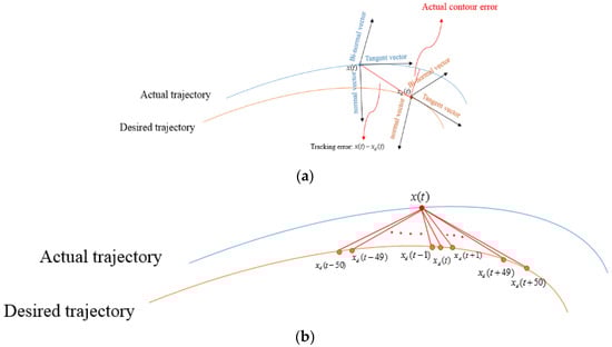
Figure 5.
Illustration of on-line contour error, (a) Concept map of contour error; and, (b) illustration of calculation actual online contour error.
Herein, a simple trajectory is adopted to finish the comparison and illustrate effectiveness of our approach. A three-dimensional desired trajectory is
where r = 1m, w = 100, sampling time is 0.0001 sec, and (m/s) denotes velocity. The corresponding result is shown in Figure 6a (blue: desired path, red: actual) and the corresponding actual and calculation contour errors are shown in Figure 6b (red: actual contour error ea, green: calculation error). We can observe that there exists error between the calculation contour error and actual contour error, but there is the same trend between calculation contour error and actual contour error; therefore, we can conclude that reducing the calculation contour error can reduce actual contour error.
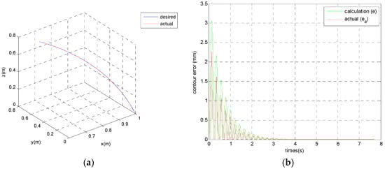
Figure 6.
Comparison of actual and calculation contour errors, (a) trajectories; (b) contour errors.
In this paper, we transfer dynamic model of linear motor system into the time-varying coordinate system in order to reduce the contour error; it illustrates that we calculate the contour in time-varying path, but the contour error is defined as the shortest distance between the current position and the entire reference trajectory, contour error is not related with time actually; therefore, we illustrate that reducing the calculation contour error can reduce actual contour error through the above simulation.
4.2. Discussion on Adaptation of Controller
In this section, we would like to illustrate the necessity of being adaptive through the discussion of system with nonlinear phenomenon. Herein, we consider that the nonlinear phenomenon includes force ripple and frictional force. The used frictional force (Ff) is the identification results of [29]
where fs = 20N, fc = 10N, and m/s, and the used force ripple is provided by the identification result of [28]. The actual mass and viscous friction coefficient are 6.2152 kg and 0.0000000001349 Ns/m, respectively. The desired trajectory in X-Y-Z axis is
where r = 0.5 m, m/s, and sampling time is 0.0001 s. Figure 7 shows the simulation results, (a) system trajectories; (b) contour errors; (c) shows the control performance of each axis; and, (d) shows the control effort of each axis, in which three cases are considered; green-line (case 1): system without Ff, Fr, and controller parameters without update; red-line (case 2): system with Ff, Fr, and controller parameters without update; black-line (case 3): system with Ff, Fr, and controller parameters with update). In addition, Table 1 introduces the performance of different case in maximum contour error, total contour error, and RMSE. From Table 1, we can clearly observe that the nonlinear phenomenon affects the performance of controller, but through the adaptive approach we can reduce the effect or nonlinear phenomenon in max error and total error. From Figure 7 and Table 1, we can find that the proposed approach performs well with small contour errors. The performances of Cases 2 and 3 can conclude that the adaption of controller is necessary for nonlinear uncertain systems.
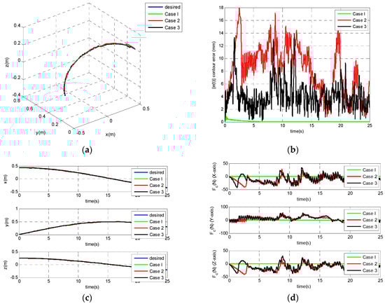
Figure 7.
Simulation results, (a) performance of different case in X-Y-Z plane, (b) contour error of different cases, (c) performance of each axis, and (d) control effort.

Table 1.
Comparison results of adaptive model-free controller.
4.3. Comparison Controller Using FNN, RFNN
Here, we compare adaptive model-free coupling control while using RFNN and FNN, where the FNN is a special case of RFNN without feedback layer. From Equation (4), dynamic model becomes complex time-vary system through transformation matrix F(t), in order to illustrate the advantage of using RFNN, a comparison results of adaptive model-free contour controller using RFNN and FNN are introduced. As far as we know, RFNN is dynamic network and is more suitable for handling time-varying problem than FNN. The desired trajectory and the initial condition are the same as above description. Figure 8 shows the simulation results (blue-line: desired trajectory; green-line: adaptive model-free coupling control using FNN). Figure 8a shows the system trajectories, Figure 8b is the corresponding contour error, and the corresponding trajectories and control efforts of each axis are shown in Figure 8c,d, respectively. Besides, Table 2 shows the performance of different case in maximum contour error, total contour error, and RMSE. Similar to the above description, from Figure 8 and Table 2, we can observe that controller using RFNN has better performance than the controller using FNN. We conclude that that RFNN is more suitable for handling time-varying problem than FNN.
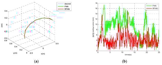
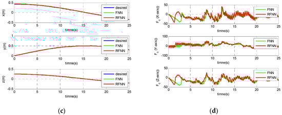
Figure 8.
Comparison results of adaptive controller using RFNN and fuzzy neural network (FNN), (a) system trajectory in X-Y-Z plane, (b) performance of contour error; (c) trajectories of each axis, (d) Control effort.
Table 2.
Comparison performance of FNN and RFNN.
5. Conclusions
We have introduced an adaptive model-free coupling controller while using RFNN for overcoming the affection of system uncertainties, force ripple, and frictional force in a three-axis CNC machine tool feed drive system, and this method did not have restrictions on the trajectories. By the concept of cross-coupling control (CCC), the considered system is transferred into a nonlinear time-varying system due to the time-dependent coordinate transformation; tangential, normal, and bi-normal components of desired contour. Herein, we propose a model-free adaptive coupling controller design approach for multi-axis linear motor system with uncertainty and nonlinear phenomena. The adaptive model-free controller design was established based on an error system by time-varying coordination transformation in order to minimize the contour errors. Specifically, an adaptive controller was developed to control for highly nonlinear system. Through the simulation results, we know that the proposed controller is effective in reducing contour error. The stability of closed-loop system is guaranteed by the Lyapunov method and the adaptation of RFNN is also obtained. Simulation results are introduced to illustrate the effectiveness.
Author Contributions
B.-S.C. and C.-H.L. initiated and developed the ideas related to this research work. Both of them developed the presented novel methods, derived relevant formulations, and carried out the performance analyses of simulation and experimental results. B.-S.C. wrote the paper draft under C.-H.L.’s guidance and Professor Lee finalized the paper. All authors have read and agreed to the published version of the manuscript.
Funding
This research received no external funding.
Acknowledgments
The authors would like to thank the Editor and reviewers for their constructive comments and suggestions. This work was supported in part by the Ministry of Science and Technology, Taiwan, under contracts MOST-108-2634-F-005-001, 107-2634-F-005-001, 106-2218-E-005-003, and 105-2221-E-005-049-MY3.
Conflicts of Interest
The authors declare no conflict of interests.
References
- Altintas, Y. Manufacturing Automation: Metal Cutting Mechanics, Machine Tool Vibrations, and CNC Design; Cambridge University Press: New York, USA, Cambridge, UK, 2012. [Google Scholar]
- Suh, S.H.; Chung, S.K.; Stround, D.H. Theory and Design of CNC Systems; Springer: Cham, Switzerland, 2008. [Google Scholar]
- Bretschneider, J.; Menzel, T. Virtual optimization of machine tools and production process. Int. J. Autom. Technol. 2007, 1, 136–140. [Google Scholar] [CrossRef]
- Koren, Y. Cross-coupled biaxial computer control for manufacturing systems. ASME Trans. J. Dyn. Syst. Meas. Control 1980, 102, 265–272. [Google Scholar] [CrossRef]
- Koren, Y.; Lo, C.C. Variable-gain cross-coupling controller for contouring. Ann. CIRP 1991, 40, 371–374. [Google Scholar] [CrossRef]
- Huang, C.H.; Lin, C.L. Evolutionary neural networks and DNA computing algorithms for dual-axis motion control. Eng. Appl. Artif. Intell. 2011, 24, 1263–1273. [Google Scholar] [CrossRef]
- Yeh, S.S.; Hsu, P.L. Estimation of the contouring error vector for the cross-coupled control design. IEEE/ASME Trans. Mechatron. 2002, 7, 44–51. [Google Scholar]
- Chen, S.L.; Wu, K.C. Contouring control of smooth paths for multi-axis motion systems based on equivalent errors. IEEE Trans. Control Syst. Technol. 2007, 15, 1151–1158. [Google Scholar] [CrossRef]
- Sencer, B.; Altintas, Y.; Croft, E. Modeling and Control of Contouring Errors for Five-Axis Machine Tools—Part I: Modeling. J. Manuf. Sci. Eng. 2009, 131, 031006. [Google Scholar] [CrossRef]
- Sencer, B.; Altintas, Y. Modeling and control of contouring errors for five-axis machine tools—Part II: Precision contour controller design. J. Manuf. Sci. Eng. 2009, 131, 031007. [Google Scholar] [CrossRef]
- Lee, J.; Dixon, W.E.; Ziegert, J.C. Adaptive nonlinear contour coupling control for a machine tool system. Int. J. Adv. Manuf. Technol. 2012, 61, 1057–1065. [Google Scholar] [CrossRef]
- Shi, R.; Lou, Y. A novel contouring error estimation for three-dimensional contouring control. IEEE Robot. Autom. Lett. 2016, 2, 128–134. [Google Scholar] [CrossRef]
- Ghaffari, A.; Galip Ulsoy, A. Dynamic contour error estimation and feedback modification for high-precision contouring. IEEE/ASME Trans. Mechatron. 2016, 21, 1732–1741. [Google Scholar] [CrossRef]
- Wang, Z.; Hu, C.; Zhu, Y.; He, S.; Zhang, M.; Haihua, M. Newton-ILC contouring error estimation and coordinated motion control for precision multiaxis systems with comparative experiments. IEEE Trans. Ind. Electron. 2018, 65, 1470–1480. [Google Scholar] [CrossRef]
- Jia, Z.J.; Ma, J.W.; Song, D.N.; Wang, F.J.; Liu, W. A review of contouring-error reduction method in multi-axis CNC machining. Int. J. Mach. Tools Manuf. 2018, 125, 34–35. [Google Scholar] [CrossRef]
- Chuang, H.Y.; Liu, C.H. Cross-coupled adaptive feedrate control for multiaxis machine tools. ASME Trans. J. Dyn. Syst. Meas. Control 1991, 113, 451–457. [Google Scholar] [CrossRef]
- Bascetta, L.; Rocco, P. Force ripple compensation in linear motors based on closed-loop position-dependent identification. IEEE/ASME Trans. Mechatron. 2010, 15, 349–359. [Google Scholar] [CrossRef]
- Shi, W.J.; Zhang, D.C. Adaptive robust control of linear motor with ripple force compensation. In Proceedings of the 2011 Third Pacific-Asia Conference on Circuits, Communications and System (PACCS), Wuhan, China, 17–18 July 2011; pp. 1–4. [Google Scholar]
- Song, F.; Liu, Y.; Xu, J.X. Iterative learning identification and compensation of space-periodic disturbance in PMLSM systems with time delay. IEEE Trans. Ind. Electron. 2018, 65, 7579–7589. [Google Scholar] [CrossRef]
- Rohrig, C.; Jochheim, A. Identification and compensation of force ripple in linear permanent magnet motors. In Proceedings of the American Control Conference, Arlington, VA, USA, 25–27 June 2001. [Google Scholar]
- Lee, C.H.; Teng, C.C. Identification and control of dynamic systems using recurrent fuzzy neural networks. IEEE Trans. Fuzzy Syst. 2000, 8, 349–366. [Google Scholar]
- Yabuta, T.; Yamada, T. Learning control using neural networks. In Proceedings of the IEEE International Conference on Robotics and Automation, Sacramento, CA, USA, 9–11 April 1991; pp. 740–745. [Google Scholar]
- Lee, C.H.; Chang, F.Y.; Lin, C.M. An efficient interval type-2 fuzzy CMAC for chaos time-series prediction and synchronization. IEEE Trans. Cybern. 2013, 44, 329–341. [Google Scholar] [CrossRef]
- Chen, H.R.; Su, K.H.; Cheng, M.Y.; Lu, J.S. Parameter-based contour error estimation for contour following accuracy improvements. In Proceedings of the 2014 International Conference on Information Science, Sapporo, Japan, 26–28 April 2014; Volume 3, pp. 1638–1642. [Google Scholar]
- Chen, C.S.; Chen, L.Y. Robost cross-coupling synchronous control by shaping position commands in multiaxes systems. IEEE Trans. Ind. Electron. 2012, 59, 4761–4773. [Google Scholar] [CrossRef]
- Sun, D. Position synchronization of multiple motion axes with adaptive coupling control. Automatica 2003, 39, 997–1005. [Google Scholar] [CrossRef]
- Sun, D. Synchronization and Control of Multiagent Systems; CRC Press, Inc.: Boca Raton, FL, USA, 2010. [Google Scholar]
- Chen, B.S. Adaptive Coupling Controller Design for Multi-Axis Systems. Master Thesis, Department of Mechanical Engineering, National Chung Hsing University, Taichung, Taiwan, 2017. [Google Scholar]
- Tan, K.K.; Huang, S.N.; Lee, T.H. Robust adaptive numerical compensation for friction and force ripple in prmanent-magnet linear motors. IEEE Trans. Magn. 2002, 38, 221–228. [Google Scholar] [CrossRef]
© 2020 by the authors. Licensee MDPI, Basel, Switzerland. This article is an open access article distributed under the terms and conditions of the Creative Commons Attribution (CC BY) license (http://creativecommons.org/licenses/by/4.0/).