COVID-19: Modeling, Prediction, and Control

Abstract

The newly emerging severe acute respiratory syndrome coronavirus 2 (SARS-CoV-2), also known as COVID-19, has been recognized as a pandemic by the World Health Organization (WHO) on 11th March 2020. There are many unknowns about this virus to date and no vaccine or conclusive treatment due to the lack of understanding of its pathogenesis and proliferation pathways which are unknown and cannot be traced. The prime objective is to stop its spread worldwide. This article aims to provide predictions of its spread using a stochastic Lotka–Volterra model coupled with an extended Kalman Filter (EKF) algorithm to model the COVID-19 dynamics. Our results show the feasibility of utilizing this model for predicting the spread of the virus and the ability of different control measures (e.g., social distancing) on reducing the number of affected people.

1. Introduction

SARS-CoV-2 known as COVID-19 is an newly emerging human infectious coronavirus that originated in Wuhan, China, and has been spreading rapidly in China and around the world since December 2019 [1]. It was declared a global emergency on 31 January 2020 by the World Health Organization (WHO) and on 11 March the disease was recognized as a global pandemic [2]. The original observation was that the virus can infect family clusters as well as in healthcare workers which confirmed the occurrence of human-to-human transmission, though the extent of this mode of transmission is unclear yet. On 21 January 2020, the WHO suggested there was possible sustained human-to-human transmission [3].

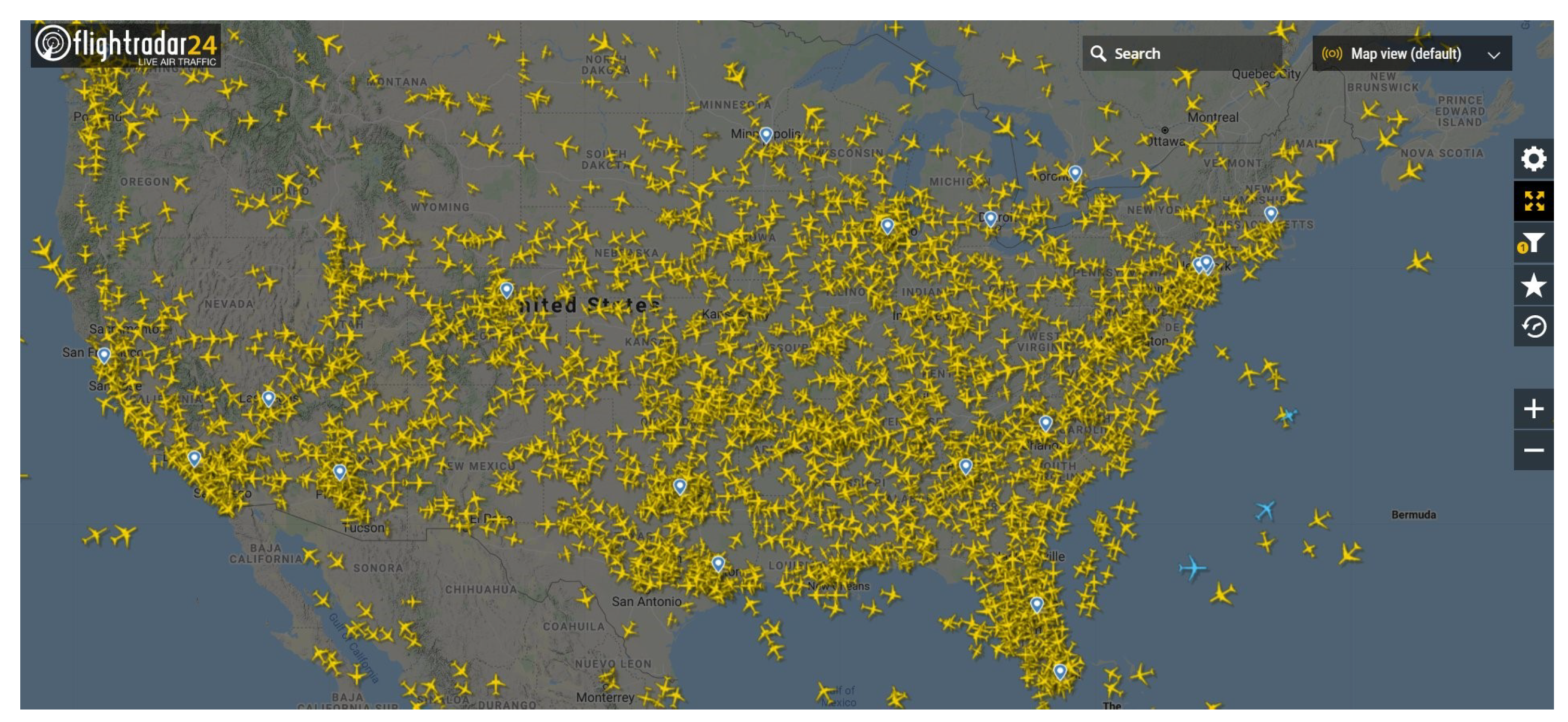
This epidemic has shocked the world and generated a significant amount of uncertainty to everyday life. Figure 1 shows a nearly empty subway station in New York City (NYC) that is typically bustling with people in normal circumstances. It also impacted the economy in an unprecedented way especially the aviation industry. Figure 2 and Figure 3 show a comparison between the skies over the US before and after the epidemic respectively and it shows an approximate 30 percent reduction in flights since the beginning of this virus and is expected to reduce even further. With this outbreak still ongoing, it has dire consequences on global public health and economics [4,5].

The number of confirmed COVID-19 cases worldwide as of 31 March 2020 is shown in Figure 4 which is collected from the WHO website. It is clear that the cases originated from China where they reached the peak at the end of February 2020 and plateaued thereafter indicating a possible control over the spread. While the US has clearly shown a dramatic increase in the number of cases recently reaching around 200,000 cases. If we track the cases day-by-day as shown in Figure 5 we cannot make any conclusion on a trend but its clear that there is an exponential increase overall worldwide. We can safely assume that given the lack of available testing kits the number could very well be much larger emphasizing the importance of resolving this manner quickly.

However, what about those people that have been infected and recovered? Those data are summarized in Figure 6 and show that people do recover from their illness and survive while others die as shown in Figure 7. The trends indicate that the number of survivals surpass the number of deaths but there are not enough data yet to make any final conclusive remarks as to the demographics of those that survive and die.

Since the outbreak is very recent there has not been many articles published on predicting the impact of variables that can reduce the total number of people infected using mathematical models. Lin et al. [8] adopted a simplified model and considered several variables including governmental actions, essential elements and others and estimated the parameters using a mechanistic model utilizing data from the 1918 influenza pandemic in England. It is not clear the variables considered have a direct relation to the outbreak nor if the trends hold true. We propose the use of a dynamical model coupled with a Kalman Filter to perform estimation of variables we considered that have recently shown to minimize the spread of the virus.

For the purpose of this article, we will utilize the data collected thus far on the pandemic to support some of the modeling calibration as will be discussed in the next sections.

2. COVID-19 Mathematical Modeling

This section presents two modeling methods to predict the spread rate of the coronavirus globally and by country. The first model utilizes the data collected thus far to build a classical power series curve fitting model. The second approach develops a dynamical model based on Lotka-Voltera equation.

2.1. Statistical Power Series Model

By incorporating all statistical data available, which were presented in Section 1, a mathematical model is developed using power series polynomials. This is a classical function approximation which can be used to extrapolate the prediction of the coronavirus spread rate. More about different sets of these classical function approximations are in [9]. We curve-fit the data as

$$y_j=\sum _{n=0}^N{a}_n{t}^n;j=0,1,\cdots ,M$$

(1)

where t is the time in days, $a_n$ are the polynomial coefficients, N is the order of the polynomial, M is the number of spread rate data points, and y is the spread rate data (given). The polynomial coefficients are evaluated using least square approximation.

The model is developed based on the considered global spread rate data in the period from 22 January to 31 March. For demonstration purposes, two data sets are modeled; (1) the global (total) confirmed cases per day, and (2) the confirmed cases per day for the USA given that it has the highest infection rate. The data sets are shown in Figure 8. The two models are used to estimate the elevation in the total number of cases per day in the next two week time frame (1–14 April). The two models can be described as

$$\begin{array}{ccc}{Y}_{\mathrm{global}}\hfill & =\hfill & t^3-78t^2+1600t-5300\hfill \\ Y_{\mathrm{USA}}\hfill & =\hfill & 0.0097t^4-t^3+33t^2-3700t+9900\hfill \end{array}$$

(2)

where t is the number of days since 22 January. If no serious control action is imposed to reduce the number of cases per day, about 171,436 confirmed cases per day is predicted in the whole world by 14 April. This number is significant and demands serious actions by leaders in order to bring this number down and flatten the curve.

This approximation model presents a good prediction to view the progressing of the cases with time. However, it does not reveal the influence of following the proper actions in the overall process. Thus, a dynamical model is needed to study how a resolution of this problem can potentially bring an end to this pandemic. The order of the polynomial is selected based on the lowest R-squared ($R^2$) value, which is a statistical measure of how close the data are to the fitted regression line. For the global case, a cubic polynomial is selected with $R^2=0.9689$. For the USA model, a 4th order polynomial is selected with $R^2=0.9816$. While the statistical models are commonly used for curve fitting applications, we believe that those two curve-fitting models would fail extrapolation beyond a period of a few days. Therefore, we are motivated to develop a dynamical model that measures most of the contributing variables in the spread rate of the virus. COVID-19 modeling and control reveals interesting challenges, not least because the data are so unreliable.

2.2. Lotka-Volterra Dynamic Model

It is well-known that dynamic models play important roles in describing the interactions among specific behaviours. We propose a new dynamic model inspired from the generalized Lotka-Volterra (gLV) model [10,11,12,13] for simulating predator-prey dynamics. The classic model has been suitably modified to build the healthy-infected individual population dynamics model. The gLV model is a first order nonlinear system of differential equations. In its discrete form, the gLV is represented as a group of first order nonlinear difference equations that relate the dissimilarity between the abundance levels of species at time t with respect to time $t-1$.

Let $\{x_i\left(t\right);i=1,\cdots ,N\}$ be the relative abundance level of the ith species at time t whose intrinsic growth rate is $g_i$. Moreover, let $c_{ij}$ represent the strength of the influence of species i onto species j (a.k.a., the ‘interaction coefficient’). Thus, the gLV model is given by:

$$\frac{\mathrm{d}}{\mathrm{d}t}{x}_i\left(t\right)=g_i{x}_i\left(t\right)+x_i\left(t\right)\sum _{j=1}^N{c}_{ij}{x}_j\left(t\right)i=1,\cdots ,N.$$

(3)

The above framework was extended to model the effects of external perturbations (e.g., antibiotics, diets) onto the microbial community structure [12,13]. This was obtained by adding another term to (3) which modulates the influence of each stimulating source into each member of the ecosystem. Mathematically, let ${ϵ}_{il}$ represent the ‘sensitivity’ of the ith species in response to lth behaviour or control action with signal strength $u_l$. The resulting gLV model is given by [13]:

$$\frac{\mathrm{d}}{\mathrm{d}t}{x}_i\left(t\right)=g_i{x}_i\left(t\right)+x_i\left(t\right)\sum _{j=1}^N{c}_{ij}{x}_j\left(t\right)+x_i\left(t\right)\sum _{l=1}^L{ϵ}_{il}{u}_l\left(t\right).$$

(4)

The proposed COVID-19 dynamical model adopts the formulation in Equation (4) where two species are considered; (1) $X_H\left(t\right)$ which is the healthy individual population at time t, (2) $X_I\left(t\right)$ is the infected individual population at time t. The population dynamics are dictated by the following differential equations:

$$\begin{array}{ccc}\frac{\mathrm{d}}{\mathrm{d}t}{X}_H\left(t\right)\hfill & =\hfill & \stackrel{\mathrm{Immigration}}{\overbrace{{\alpha }^H{X}_H}}-\stackrel{\mathrm{Infection}}{\overbrace{\beta X_H{X}_I}}+\stackrel{\mathrm{Recovery}}{\overbrace{\gamma X_I}}+\stackrel{\mathrm{Control}}{\overbrace{X_H{\displaystyle \sum _{i=1}^N}{ϵ}_i^H{U}_i}}\hfill \\ \frac{\mathrm{d}}{\mathrm{d}t}{X}_I\left(t\right)\hfill & =\hfill & \underset{\mathrm{Immigration}}{\underbrace{{\alpha }^I{X}_I}}+\underset{\mathrm{Infection}}{\underbrace{\beta X_H{X}_I}}-\underset{\mathrm{Recovery}}{\underbrace{\gamma X_I}}-\underset{\mathrm{Control}}{\underbrace{X_I{\displaystyle \sum _{i=1}^N}{ϵ}_i^I{U}_i}}-\underset{\mathrm{Death}}{\underbrace{\delta X_I}}\hfill \end{array}$$

(5)

The population dynamics represent five different states of interaction as follows:

• Immigration: This due to the individual travels between different zones. When people move from a destination to another destination (of interest), the size of the population in the destination will increase linearly. ${\alpha }^H⩾0$ and ${\alpha }^I⩾0$ are the immigration rates of healthy individuals and infected individuals, respectively. For example, the travel bans between different destinations means that the values of immigration rates are zero. It is obvious that ${\alpha }^H⩽0$ and ${\alpha }^I⩽0$ when the individuals travel out of the destination. This implies that the size of the population will decrease.
• Infection: This due to the direct interactions between the healthy individuals and infected individuals. $\beta ⩾0$ is the infection rate. The negative sign in the healthy population term indicates that the infection will reduce the number of healthy individuals which are, in turn, added to the infected population. The infection rate can be managed by reducing the interactions between healthy and infected individuals. Which in a perfect world when we have everyone adhere to social distancing, $\beta$ can be simply zero.
• Recovery: This indicates the infected individuals who got recovered and cured based on their self immunization; no medication was used. This population will be added to the healthy population. $\gamma ⩾0$ is the cure rate. We have no control cure rate since no medication or vaccine is available thus far. Figure 9 represents the global percentage of death (and recovered) cases relative to the total confirmed cases per day. The data represent the cases from 22 January until 31 March. These data can help quantify the value of $\gamma$ that can be considered in this model. The global mean value is $25.5\%$.
• Control: This indicates any possible control that can by imposed by governments. The control actions can be categorized into two aspects. First, the effectiveness of any potential vaccine to avoid infection of COVID-19 or potential medication to treat infected cases. The vaccine control is measured by ${ϵ}^H⩾0$, which will lead to an increase in the size of the healthy population. Whereas, the medication treatment is measured by ${ϵ}^I⩾0$. Thus, the control term can be modified as $X_H{\sum }_{i=1}^N{ϵ}_i^H{U}_i-X_I{\sum }_{i=1}^N{ϵ}_i^I{U}_i$ for the healthy population, and $X_I{\sum }_{i=1}^N{ϵ}_i^I{U}_i-X_H{\sum }_{i=1}^N{ϵ}_i^H{U}_i$ for the infected population. Since, no vaccine or medication is available to treat the COVID-19 cases, we can consider ${ϵ}^H={ϵ}^I=0$. Second, the control actions can be represented in terms of guidelines provided by the World Health Organization to reduce the spread of the coronavirus. Currently, there are five guidelines recommended by the World Health Organization to stop the spread of the coronavirus, see Figure 10.
  Thus the control actions can be given by

  $$U_i\left(t\right)={\left[\begin{array}{ccccc}{U}_{\mathrm{HANDS}}& U_{\mathrm{ELBOW}}& U_{\mathrm{FACE}}& U_{\mathrm{SPACE}}& U_{\mathrm{HOME}}\end{array}\right]}^{T}i=1,\cdots ,5.$$

  (6)
  For demonstration purposes and due to the lack of data available to model these control behaviours, we consider a single normalized control action that is a contribution of all the above five guidelines in our model. Therefore, we can define:

  $$U=\sqrt{U_{HANDS}^2+U_{ELBOW}^2+U_{FACE}^2+U_{SPACE}^2+U_{HOME}^2}$$

  (7)

  and $ϵ=\sqrt{{\sum }_{i=1}^{N=5}{ϵ}_i^2}$. We suggest the normalization because there are no adequate data to analysis for each variable. We keep the main terms for future reference, when more reliable data become available. The normalization is only for demonstration purposes and is not practical without having sufficient and reliable data.
• Death: This indicates the infected individuals who died. $\delta ⩾0$ is the death rate. Figure 9 represents global percentage of recovered (and death) cases relative to the total confirmed cases per day. This data will help quantify the values of $\delta$ that can be considered in this model. The global mean value is $3.22\%$.

The population dynamic model in Equation (5) is not a unique representation of the COVID-19 healthy/infected populations. Some terms can be modified or added depending on the study and prospective for the problem. We present this model as a good candidate to overview the dynamic behaviour of the coronavirus spread rate. By utilizing the dynamic model in Equation (5), one can get an understanding of how to reduce the infected populations. In the dynamic model, the values of $\gamma$ and $\delta$ are uncontrollable and can be estimated using the statistical data in Figure 9. However, the values of ${\alpha }^H$, ${\alpha }^I$, $\beta$, ${ϵ}^H$, and ${ϵ}^I$ are controllable. Working to minimize the values of ${\alpha }^H$, ${\alpha }^I$, $\beta$ as well as maximizing the values of ${ϵ}^H$, and ${ϵ}^I$ will improve the situation and result in less number of infected people. The optimum case is ${\alpha }^H={\alpha }^I=\beta =0$, ${ϵ}^H={ϵ}_{\max }^H$, and ${ϵ}^I={ϵ}_{\max }^I$.

We observe that the dynamic model in Equation (5) has missed the growth rate of the overall population. In other words, the model needs to be augmented to account for the fertility rate and (normal or non COVID-19) death rate. Thus, the augmented model is given by

$$\begin{array}{ccc}\frac{\mathrm{d}}{\mathrm{d}t}{X}_H\left(t\right)\hfill & =\hfill & \stackrel{\mathrm{Immigration}}{\overbrace{{\alpha }^H{X}_H}}-\stackrel{\mathrm{Infection}}{\overbrace{\beta X_H{X}_I}}+\stackrel{\mathrm{Recovery}}{\overbrace{\gamma X_I}}+\stackrel{\mathrm{Birth}}{\overbrace{{\eta }^H{X}_H}}-\stackrel{\mathrm{Death}}{\overbrace{{\delta }^H{X}_H}}+\stackrel{\mathrm{Control}}{\overbrace{X_H{\displaystyle \sum _{i=1}^N}{ϵ}_i^H{U}_i}}\hfill \\ \frac{\mathrm{d}}{\mathrm{d}t}{X}_I\left(t\right)\hfill & =\hfill & \underset{\mathrm{Immigration}}{\underbrace{{\alpha }^I{X}_I}}+\underset{\mathrm{Infection}}{\underbrace{\beta X_H{X}_I}}-\underset{\mathrm{Recovery}}{\underbrace{\gamma X_I}}+\underset{\mathrm{Birth}}{\underbrace{{\eta }^I{X}_I}}-\underset{\mathrm{Death}}{\underbrace{{\delta }^I{X}_I}}-\underset{\mathrm{Control}}{\underbrace{X_I{\displaystyle \sum _{i=1}^N}{ϵ}_i^I{U}_i}}\hfill \end{array}$$

(8)

where ${\eta }^H$ and ${\eta }^I$ are the fertility rate in the healthy and infected individuals. ${\delta }^H$ and ${\delta }^I$ are the death rate in the healthy and infected individuals. Note that these parameters are uncontrollable and can be estimated from statistical data. Perhaps, finding an effective medicines, vaccines or anti viral, and adequate ventilators would control the death rate ${\delta }^I$ of the infected population and lead to less death cases.

The state-space dynamic population model is defined by

$$\dot{\mathit{x}}\left(t\right)=A\mathit{x}+{\mathit{f}}_1\left(\mathit{x}\right)+{\mathit{f}}_2\left(\mathit{x}\right)\mathit{u}$$

(9)

where $\mathit{x}\left(t\right)=\left[\begin{array}{c}{X}_H\left(t\right)\\ X_I\left(t\right)\end{array}\right]$, $A=\left[\begin{array}{cc}{\alpha }^H+{\eta }^H-{\delta }^H& \gamma \\ 0& {\alpha }^I-\gamma +{\eta }^I-{\delta }^I\end{array}\right]$, ${\mathit{f}}_1\left(\mathit{x}\right)=\left[\begin{array}{c}-\beta x_1{x}_2\\ \beta x_1{x}_2\end{array}\right]$, ${\mathit{f}}_2\left(\mathit{x}\right)=\left[\begin{array}{c}{x}_1{\left[{ϵ}^H\right]}^T\\ x_1{\left[{ϵ}^I\right]}^T\end{array}\right]$, $\mathit{u}\left(t\right)=\left[\begin{array}{c}{U}_1\\ U_2\\ ⋮\\ U_N\end{array}\right]$, and ${ϵ}^T=[{ϵ}_1{ϵ}_2\cdots {ϵ}_N]$.

3. Extended Kalman Filter

The main drawbacks of this model include the fact that the model can only consider the measurement noise without taking into consideration uncertainties in the underlying dynamics. Therefore, we develop a stochastic gLV model with Extended Kalman Filter (EKF) algorithm to model COVID-19 spread dynamics.

The nonlinear dynamic stochastic model that captures the COVID-19 spread rate along with the measurement model is defined as:

$$\begin{array}{ccc}\hfill \frac{\mathrm{d}}{\mathrm{d}t}{x}_i\left(t\right)\equiv \dot{\mathit{x}}& =& \mathit{f}\left(\mathit{x}\right(t),\mathit{u}(t\left)\right)+G\left(t\right)\mathit{w}\left(t\right)\hfill \\ \hfill y_i\left(t\right)\equiv \mathit{y}& =& \mathit{h}\left(\mathit{x}\right(t),t)+\mathit{v}\left(t\right)\hfill \\ \hfill i& =& 1,2,\cdots ,N\hfill \end{array},$$

(10)

where N denotes the number of state variables (i.e., $N=2$ in the model), $\mathit{x}\left(t\right)\in {\Re }^N$ is the system state vector, $\mathit{y}\left(t\right)\in {\Re }^N$ stands for the observation vector. The nonlinear state model is defined by $\mathit{f}:{\Re }^N\to {\Re }^N$, which is the discrete-time form of Equation (9). The nonlinear observation model is defined by $\mathit{h}:{\Re }^N\to {\Re }^R$. $G\left(t\right)$ is a coefficient matrix associated with the process noise. $\mathit{w}\left(t\right)\sim \mathcal{N}(0,Q(t\left)\right)$ and $\mathit{v}\left(t\right)\sim \mathcal{N}(0,R(t\left)\right)$ represent the zero-mean Gaussian uncorrelated white-noise process and measurements, respectively, with covariance matrices given by

$$\begin{array}{ccc}\hfill E\left\{\mathit{w}\left(t_2\right){\mathit{w}}^T\left(t_1\right)\right\}& =& Q\left(t_2\right)\delta \left(t_2-t_1\right)\hfill \\ \hfill E\left\{\mathit{v}\left(t_2\right){\mathit{v}}^T\left(t_1\right)\right\}& =& R\left(t_2\right)\delta \left(t_2-t_1\right)\hfill \\ \hfill E\left\{\mathit{w}\left(t_2\right){\mathit{v}}^T\left(t_1\right)\right\}& =& 0\hfill \\ \hfill \delta (t_i,t_j)& =& \left\{\begin{array}{cc}0\hfill & \mathit{if}i\ne j\hfill \\ 1\hfill & \mathit{if}i=j\hfill \end{array}\right.\hfill \end{array}$$

(11)

where $E\{.\}$ is the expectation operator. The EKF structure for the state estimate $\widehat{\mathit{x}}$, in the absence of the control input, is given by

$$\dot{\widehat{\mathit{x}}}\left(t\right)=\mathit{f}(\widehat{\mathit{x}}\left(t\right),t)+K\left(t\right)[\mathit{y}\left(t\right)-\mathit{h}\left(t\right)\left(\widehat{\mathit{x}}\left(t\right)\right)]$$

(12)

where $K\left(t\right)$ represents the Kalman gain. [14] provides detailed derivations of the EKF. The state vector is augmented to estimate both the dynamic states and the unknown parameters. We consider the following augmented state vector $\mathit{z}\left(t\right)$ to estimate both the model states $\mathit{x}\left(t\right)$ and parameters $\mathit{p}\left(t\right)$

$$\mathit{z}\left(t\right)=\left[\begin{array}{c}\mathit{x}\left(t\right)\\ \mathit{p}\end{array}\right].$$

(13)

Therefore, the augmented system becomes

$$\begin{array}{ccc}\hfill \dot{\mathit{z}}\left(t\right)& =& \mathit{F}\left(\mathit{z}\right(t\left)\right)+\mathit{\zeta }\left(t\right)\hfill \\ \hfill \mathit{y}\left(k\right)& =& \mathit{h}\left(\mathit{z}\right(t\left)\right)+\mathit{v}\left(t\right)\hfill \end{array},$$

(14)

where $\mathit{\zeta }\left(t\right)$ denotes the zero-mean Gaussian white-noise for the augmented dynamic, and

$$\begin{array}{ccc}\hfill \mathit{F}\left(\mathit{z}\right(t),\mathit{p})& =& \left[\begin{array}{c}\mathit{f}\left(\mathit{x}\right(t),\mathit{p})\\ 0\end{array}\right]\hfill \\ \hfill \mathit{h}\left(\mathit{z}\right(t\left)\right)& =& \mathit{h}\left(\mathit{x}\right(t),\mathit{p})\hfill \end{array}.$$

(15)

For our gLV dynamic model, the observation model is defined as

$$\mathit{y}=\mathit{x}\left(t\right)+\mathit{v}\left(t\right).$$

(16)

The system parameters are given by

$$\mathit{p}={\left[{\alpha }^H,{\alpha }^I,\beta ,\gamma ,\delta \right]}^T.$$

(17)

The EKF is implemented following sequentially the steps below:

• Initialization: at $k=0$ and for given initial states ${\mathit{z}}_0={[{\mathit{x}}_0,{\mathit{p}}_0]}^T$, the initial value of the covariance matrix is given by:

  $$P_0=\left[\begin{array}{cc}{P}_{x_0{x}_0}& P_{x_0{p}_0}\\ P_{p_0{x}_0}& P_{p_0{p}_0}\end{array}\right]$$

  (18)

  and

  $$\begin{array}{ccc}\hfill {\widehat{\mathit{z}}}^{-}\left(0\right)& =& E\left\{\mathit{z}\left(0\right)\right\}={\mathit{z}}_0\hfill \\ \hfill P^{-}\left(0\right)& =& E\left\{(\mathit{z}\left(0\right)-{\mathit{z}}_0){(\mathit{z}\left(0\right)-{\mathit{z}}_0)}^T\right\}=P_0\hfill \end{array}$$

  (19)

  where the superscript (−) denotes a priori value. The initial covariance matrices are given by

  $$\begin{array}{ccc}\hfill P_{x_0{x}_0}& =& E\left\{(\mathit{x}\left(0\right)-{\mathit{x}}_0){(\mathit{x}\left(0\right)-{\mathit{x}}_0)}^T\right\}\hfill \\ \hfill P_{x_0{p}_0}& =& E\left\{(\mathit{x}\left(0\right)-{\mathit{x}}_0){(\mathit{p}\left(0\right)-{\mathit{p}}_0)}^T\right\}\hfill \\ \hfill P_{p_0{x}_0}& =& E\left\{(\mathit{p}\left(0\right)-{\mathit{p}}_0){(\mathit{x}\left(0\right)-{\mathit{x}}_0)}^T\right\}\hfill \\ \hfill P_{p_0{p}_0}& =& E\left\{(\mathit{p}\left(0\right)-{\mathit{p}}_0){(\mathit{p}\left(0\right)-{\mathit{p}}_0)}^T\right\}\hfill \end{array}.$$

  (20)
  Assume that $\mathit{z}\left(0\right)\sim \mathcal{N}(0,P(0\left)\right)$.
• Gain: compute the Kalman gain matrix

  $$\begin{array}{cc}\hfill K\left(k\right)=& P^{-}\left(k\right)H^T\left({\widehat{\mathit{z}}}^{-}\left(k\right)\right)\hfill \\ \hfill & [H\left({\widehat{\mathit{z}}}^{-}\left(k\right)\right)P^{-}\left(k\right)H^T{({\widehat{\mathit{z}}}^{-}\left(k\right)+R\left(k\right)]}^{-1},\hfill \end{array}$$

  (21)

  where $H\left({\widehat{\mathit{z}}}^{-}\left(k\right)\right)\equiv \frac{\partial \mathit{h}}{\partial \mathit{z}}{|}_{{\widehat{\mathit{z}}}^{-}\left(k\right)}$.
• Update: update the state estimate ${\widehat{\mathit{z}}}^{+}\left(k\right)$ and covariance $P^{+}\left(k\right)$ at each measurement

  $$\begin{array}{ccc}\hfill {\widehat{\mathit{z}}}^{+}\left(k\right)& =& {\widehat{\mathit{z}}}^{-}\left(k\right)+K\left(k\right)[\mathit{y}\left(k\right)-h\left({\widehat{\mathit{z}}}^{-}\left(k\right)\right)]\hfill \\ \hfill P^{+}\left(k\right)& =& [I-K\left(k\right)H\left({\widehat{\mathit{z}}}^{-}\left(k\right)\right)]P^{-}\left(k\right)\hfill \end{array},$$

  (22)

  where the superscript (+) denotes posteriori value.
• Propagation: propagate both the state estimate $\widehat{\mathit{z}}\left(k\right)$ and covariance $P\left(k\right)$ using the posteriori estimate ${\widehat{\mathit{z}}}^{+}\left(k\right)$ and posteriori covariance $P^{+}\left(k\right)$

  $$\begin{array}{ccc}\hfill {\widehat{\mathit{z}}}^{-}(k+1)& =& F({\widehat{\mathit{z}}}^{+}\left(k\right),u\left(k\right))\hfill \\ \hfill P^{-}(k+1)& =& \mathsf{\Phi }\left({\widehat{\mathit{z}}}^{+}\left(k\right)\right)P^{+}\left(k\right){\mathsf{\Phi }}^T\left({\widehat{\mathit{z}}}^{+}\left(k\right)\right)+Q\left(k\right)\hfill \end{array}.$$

  (23)

  where $\mathsf{\Phi }\left({\widehat{\mathit{z}}}^{+}\left(k\right)\right)\equiv \frac{\partial \mathit{F}\left(\mathit{z}\right)}{\partial \mathit{z}}{|}_{{\widehat{\mathit{z}}}^{+}\left(k\right)}$.

The implementation of the above algorithm is conducted on a set of generated data to demonstrate the convergence and how the model parameters are computed. The stochastic data are generated based on nominal values of case 1 in

Table 1. Test cases used to evaluate the model.

Case	${\mathit{\alpha }}^{\mathit{H}}$	${\mathit{\alpha }}^{\mathit{I}}$	$\mathit{\beta }$	$\mathit{\gamma }$	${\mathit{\eta }}^{\mathit{H}}$	${\mathit{\eta }}^{\mathit{I}}$	${\mathit{\delta }}^{\mathit{H}}$	${\mathit{\delta }}^{\mathit{I}}$
1	0	0	0	0.25	0.01	0	0.001	0.05
2	0.001	0.001	0.005	0.25	0.01	0	0.010	0.05
3	0.001	0.001	0.050	0.25	0.01	0	0.010	0.05
4	0	0	vary	0.25	0.05	0.025	0.010	0.05
5	0	0.100	control	0.25	0.01	0.010	0.010	0.05

. Figure 11 exhibits how the system parameters converge to the estimated values. Thus, the dynamic model can now predict the dynamic behaviour of the infection in a particular area or country. Next section, takes this model and introduces control strategies to resolve the inflation in the infection population of COVID-19.

4. Control Authority and Regulation

This section discusses how to apply control strategies to the mathematical model, in Equation (8), and predict the best actions and their influence to slow down the spread rate of the coronavirus.

There are two control schemes that are proposed to interact with the population model and provide system stability by reducing the number of infected cases per day, as shown in Figure 12. First, the high level control represents the effectiveness of any potential vaccine to avoid infection of COVID-19 or potential medication to treat infected cases. Both control inputs are tuned to decrease the size of the infected population to the desired reference, zero infection. Second, the low level control represents the actions that individuals should follow to reach to the same desired reference.

Since there is no vaccine nor medication that has been proven to protect or treat individuals from this disease, let us discuss how other model parameters provide control on the spread rate. In the dynamic model, the values of $\gamma$, $\eta$, and $\delta$ are uncontrollable and are normally estimated using the statistical data. However, the values of ${\alpha }^H$, ${\alpha }^I$, and $\beta$ are controllable. Working to minimize the values of ${\alpha }^H$, ${\alpha }^I$, and $\beta$ improves the situation and results in less number of infected population. Optimum case is ${\alpha }^H={\alpha }^I=\beta =0$. Let us simulate the dynamics by tuning these variables and investigate the effect in the healthy and infected populations. Based on the statistical data available, we ran experimental simulation for five test cases described below and shown in Table 1 and Figure 13. We assume that country (A) has 100 people total population with $50\%$ infected with COVID-19.

Case 1 investigates the impact of the infection rate $\beta$ on the population (e.g., the country imposes a travel ban and no immigration allowed). As shown in Figure 13a, country (A) could reach to zero infected cases in less than two weeks if it controlled the infection rate ($\beta =0$); e.g., social distancing. However in case 2, the country might need about three months to reach a steady state zero infection if it allowed infection rate and immigration to continue as is, as shown in Figure 13b. Case (3) shows the extreme condition when higher infection rate is allowed. Thus, the majority of the population got infected in the first week before the entire population dropped to small numbers due to the death rate, as shown in Figure 13c. Note that we assumed that any recovered case could still get the infection if it was exposed to infected individuals. Case 4 investigates the infected population changes to different values of the infection rate. It is clear in Figure 13d that the infected population increased with the increase of the infection rate. The elevation reached the peak at earlier week, when the entire community got infected. Then, the population started dropping down due to the increase in death rate.

It is very clear that ($\beta$) plays a significant role in controlling the spread rate and the infected population system. $\beta$ embodies all parameters that relate to guidelines recommended by the world health organization, most importantly social distancing. The value of $\beta$ may vary from country to country, region to region, and culture to culture. However, the best practice is driving this value to a minimum with time. This is the low level control scheme that assumes the infection rate as a function of the infected population. In control theory, it is called closed-loop feedback control law. Now, $\beta$ is treated as a control input that directly depends on the infected population. It is given as

$${\beta }^{*}=-K{X}^I$$

(24)

where K is the control gain that can be tuned based on the country capability to implement the WHO guidelines; control authority. Figure 14 exhibits Case 5 (in Table 1) that shows the response of the population dynamical system to the feedback control with different value of control gains. It is clear that imposing strict control authority in the infection rate would lead to a quick elimination of the disease. On the contrary, lean control practices of isolation and social distancing will delay the process and may lead to instability as shown in case 3.

5. Conclusions

The paper presented a dynamical model utilizing both the Lotka–Volterra model coupled with an extended Kalman Filter in order to evaluate the spread of COVID-19 and ways to control that spread. Initially, data were collected to understand the scope of the spread worldwide in order to aid in calibrating the model to ensure accuracy. Five distinct state variables were considered that were shown to be crucial in spreading the virus that include the immigration of people from country to country, infection rate at any specific location, number of recoveries from the virus, control measures imposed by governments to limit the spread, and death rates. It was shown that without imposing any control measures the spread grows exponentially while the spread can be controlled within several weeks if a complete travel ban was implemented to prevent the spread. The impact of social distancing was the most prominent among all other variables and has proven to reduce the spread when comparing to actual data from states nationwide. While a simplified statistical model utilizing a power series is capable of making predictions based on historical data, studying the impact of control measures is not adequate and a dynamical model offers the ability to perform such evaluations which should be considered for future prediction models during such pandemics. The model can be further expanded to add other state variables that can impact the virus spread and evaluate its effectiveness in real time.

References

1. Rismanbaf, A. Potential Treatments for COVID-19; a Narrative Literature Review. Arch. Acad. Emerg. Med. 2020, 8, e29. [Google Scholar] [PubMed]
2. Coronavirus Disease (COVID-19) Pandemic. 2020. Available online: https://www.who.int/emergencies/diseases/novel-coronavirus-2019 (accessed on 29 March 2020).
3. Available online: https://twitter.com/WHOWPRO/status/1219478547644813312?s=20 (accessed on 27 March 2020).
4. Bogoch, I.I.; Watts, A.; Thomas-Bachli, A.; Huber, C.; Kraemer, M.U.G.; Khan, K. Pneumonia of unknown aetiology in Wuhan, China: Potential for international spread via commercial air travel. J. Travel Med. 2020, 27, taaa008. [Google Scholar] [CrossRef]
5. Wu, J.; Leung, K.; Leung, G. Nowcasting and forecasting the potential domestic and international spread of the 2019-nCoV outbreak originating in Wuhan, China: A modelling study. Lancet 2020, 395, 689–697. [Google Scholar] [CrossRef] [Green Version]
6. 13 Photos of New York City Looking Deserted as the City Tries to Limit the Spread of the Coronavirus. 2020. Available online: https://www.businessinsider.com/coronavirus-pictures-of-new-york-city-empty-streets-2020-3#empty-street-is-seen-in-manhattan-borough-following-the-outbreak-of-coronavirus-disease-covid-19-in-new-york-city-us-mar-15-2020-13 (accessed on 29 March 2020).
7. Flight Tracking Statistics. 2020. Available online: https://www.flightradar24.com/data/statistics (accessed on 27 March 2020).
8. Lin, Q.; Zhao, S.; Gao, D.; Lou, Y.; Yang, S.; Musa, S.; Wang, M.; Cai, Y. A conceptual model for the coronavirus disease 2019 (COVID-19) outbreak in Wuhan, China with individual reaction and governmental action. Int. J. Infect. Dis. 2020, 93, 211–216. [Google Scholar] [CrossRef] [PubMed]
9. Bani-Younes, A. Orthogal Polynomial Approximation in Higher Dimensions: Applications in Astrodynamics. Ph.D. Thesis, Texas A&M University, College Station, TX, USA, 2013. [Google Scholar]
10. Lotka, A.J. Contribution to the Theory of Periodic Reactions. J. Phys. Chem. 1910, 14, 271–274. [Google Scholar] [CrossRef] [Green Version]
11. Goel, N.S.; Maitra, S.C.; Montroll, E.W. On the Volterra and Other Nonlinear Models of Interacting Populations. Rev. Mod. Phys. 1971, 43, 231–276. [Google Scholar] [CrossRef]
12. Alshawaqfeh, M.; Serpedin, E.; Bani Younes, A. Inferring microbial interaction networks from metagenomic data using SgLV-EKF algorithm. BMC Genom. 2017, 18, 228. [Google Scholar] [CrossRef] [PubMed] [Green Version]
13. Stein, R.R.; Bucci, V.; Toussaint, N.C.; Buffie, C.G.; Rätsch, G.; Pamer, E.G.; Sander, C.; Xavier, J.B. Ecological modeling from time-series inference: Insight into dynamics and stability of intestinal microbiota. PLoS Comput. Biol. 2013, 9, e1003388. [Google Scholar] [CrossRef] [PubMed]
14. Crassidis, J.; Junkins, J. Optimal Estimation of Dynamic Systems; Chapman & Hall/CRC Applied Mathematics & Nonlinear Science; CRC Press: Boca Raton, FL, USA, 2011. [Google Scholar]
Figure 1. People enter a nearly empty Fulton subway station during the evening rush, as people react to coronavirus disease in New York City, U.S., 18 March 2020 [6].
Applsci 10 03666 g001
Figure 2. Commercial flight traffic above the US pre COVID-19 outbreak, 1 March 2020 [7].
Applsci 10 03666 g002
Figure 3. Commercial flight traffic above the US post COVID-19 outbreak showing a 30 percent reduction, 29 March 2020 [7].
Applsci 10 03666 g003
Figure 4. Time series of global confirmed cases of COVID-19 from 22 January to 31 March.
Applsci 10 03666 g004
Figure 5. Number of daily confirmed cases by country of COVID-19 from 22 January to 31 March.
Applsci 10 03666 g005
Figure 6. Time series of global recovered cases of COVID-19 from 22 January to 31 March.
Applsci 10 03666 g006
Figure 7. Time series of global death cases of COVID-19 from 22 January to 31 March.
Applsci 10 03666 g007
Figure 8. Number of daily confirmed cases of COVID-19 from 22 January to 31 March and the prediction based on the statistical power series model in the following projected two weeks (until 14 April).
Applsci 10 03666 g008
Figure 9. The global death (and recovered) to confirmed ratio of COVID-19 from 22 January to 31 March.
Applsci 10 03666 g009
Figure 10. The general five guidelines recommended by the World Health Organization to stop the spread of the coronavirus.
Applsci 10 03666 g010
Figure 11. The Extended Kalman Filter (EKF) estimated parameters used for the predictions.
Applsci 10 03666 g011
Figure 12. Low level and high level control structure considered in this paper.
Applsci 10 03666 g012
Figure 13. Experimental results based on the assumed 100 subjects evaluated for this study.
Applsci 10 03666 g013
Figure 14. Tuning the control gain.
Applsci 10 03666 g014