Article

Quality Assessment by Region and Land Cover of Sharpening Approaches Applied to GF-2 Imagery

1
State Key Laboratory of Resources and Environmental Information System, Institute of Geographic Sciences and Natural Resources Research, Chinese Academy of Sciences, Beijing 100101, China
2
Jiangsu Center for Collaborative Innovation in Geographical Information Resource Development and Application, Nanjing 210023, China
*
Author to whom correspondence should be addressed.
Appl. Sci. 2020, 10(11), 3673; https://doi.org/10.3390/app10113673
Submission received: 7 May 2020 / Revised: 22 May 2020 / Accepted: 22 May 2020 / Published: 26 May 2020
(This article belongs to the Section Earth Sciences)

Abstract

:
The existing pansharpening methods applied to recently obtained satellite data can produce spectral distortion. Therefore, quality assessments should be performed to address this. However, quality assessment of the whole image may not be sufficient, because major differences in a given region or land cover can be minimized by small differences in another region or land cover in the image. Thus, it is necessary to evaluate the performance of the pansharpening process for different regions and land covers. In this study, the widely used modified intensity-hue-saturation (mIHS), Gram–Schmidt spectral sharpening (GS), color spectral sharpening (CN), and principal component analysis (PCA) pansharpening methods were applied to Gaofen 2 (GF-2) imagery and evaluated according to region and land-cover type, which was determined via an object-oriented image analysis technique with a support vector machine-supervised method based on several reliable quality indices at the native spatial scale without reference. Both visual and quantitative analyses based on region and land cover indicated that all four approaches satisfied the demands for improving the spatial resolution of the original GF-2 multispectral (MS) image, and mIHS produced results superior to those of the GS, CN, and PC methods by preserving image colors. The results indicated differences in the pansharpening quality among different land covers. Generally, for most land-cover types, the mIHS method better preserved the spectral information and spatial autocorrelation compared with the other methods.

1. Introduction

Different types of features and land covers in remotely sensed imagery can be detected by comparing their responses over spectral bands [1]. Most optical Earth observation satellites, such as Landsat, Sentinel-2, SPOT 5, QuickBird, IKONOS, GeoEye-1, WorldView-2, China-Brazil Earth Resource Satellite (CBERS) 4, Gaofen 1 (GF-1), and Gaofen 2 (GF-2), image the Earth’s surface with two types of sensors having different spatial resolutions, e.g., high-spatial resolution panchromatic (PAN) and low-spatial resolution multispectral (MS) sensors, with consideration of sensor hardware limitations, satellite data transmission, satellite life, image processing time, and space costs [2,3,4]. However, many remote-sensing applications require a single image with high spatial and spectral resolutions for the effective classification of features, land covers, etc. [2,5]. To address this challenge, merging remote-sensing images with different spatial resolutions is a key process [6]. This process is known as pansharpening in the field of remote sensing and can be performed at the pixel, feature, or decision level [7]. The details of popular and state-of-the-art pansharpening methods in these three levels were reviewed and explained by Ghassemian [7]. Pansharpening methods at the pixel level are the mainstream approaches and are popularly applied in practice. Some have been embedded in commercial remote-sensing image processing systems such as ENVI, ERDAS Imagine, and PCI Geomatica. The representational methods are the modified intensity-hue-saturation (mIHS), principal component analysis (PCA), color spectral sharpening (CN), and Gram–Schmidt spectral sharpening (GS) approaches [8,9,10,11,12,13]. However, numerous problems make pansharpening challenging, and no single pansharpening method can deal with all of them [14,15].
The widespread application of many different pansharpening approaches has increased the importance of evaluating the quality of pansharpened images [7,16]. Existing pansharpened image quality assessment methods employ many different quality metrics for both qualitative (visual analysis) and quantitative (objective analysis with and without a reference image) evaluations [7,17]. The available quality metrics were reviewed in previous studies [2,7,16,18,19]. Of course, the classification accuracy can also be used to compare the quality of the pansharpened images derived from the various pansharpening methods [6,20,21,22,23]. However, this quality assessment method is seldom used, because it cannot provide the spectral, spatial, and radiometric quality of the pansharpened image separately. Quantitatively assessing image pansharpening is challenging because of the different application demands and the absence of a clearly defined ideal reference image [7,24,25]. There are two main approaches for evaluating the quality of the pansharpened image without a reference image. The first approach considers the original MS image as a reference and evaluates the quality of the pansharpened image by calculating the differences between the original MS image and the downsampled pansharpened MS image using the proposed spatial and spectral quality indices. This approach operates on an image at the downsampled scale, but the quality of the pansharpened images derived from the different pansharpening methods depends on the spatial scale and the imaging sensor, and the performance of the assessment at the downsampled scale may not be the same as that at the full scale [26]. Quality assessment of pansharpened image through downsampling of the original PAN and MS images is not suitable for high-resolution images; quality assessment should be performed in full resolution [27]. The second approach focuses on the relationships among the original and pansharpened images. This approach directly operates on the image at the native scale, but the quality metrics may affect the assessment results [7]. Despite the questionable assumption of scale invariance for pansharpening performance [26], several reliable quality indices can be used, including global statistics such as the mean, standard deviation (STDEV), entropy (EN), and average gradient (AG) [18,19,22].
Quality assessment of the different image pansharpening methods is traditionally performed for the whole scene through quality metrics calculated pixel-by-pixel or region-by-region. However, this method is not only tedious and slow but also unsuitable for the assessment of regions that contain complementary information in PAN and MS images [28]. Additionally, it cannot evaluate the similarities of features and land covers between the original and pansharpened MS images. Hence, quality assessment by land cover is a promising approach that facilitates the analysis of the effects of pansharpening methods across different features and land covers [15]. However, to date, research has only focused on a few types of land covers, such as soil, water, and crops [15], and the responses of different land covers to pansharpening methods require further study. Therefore, it is necessary to evaluate the performance of the pansharpening process for more land covers.
Spectral distortion is a significant issue when existing pansharpening methods are used with imagery captured by new satellites [29]. This may be due to the different spectral ranges, different spectral resolutions of the MS bands, and the difference in the spectral ranges between the PAN and MS bands. Hence, quality assessment of existing pansharpening methods applied to images recently captured by new satellites should also be performed. Many researchers have evaluated the performance of pansharpening methods on Landsat, Sentinel-2, SPOT 5, QuickBird, IKONOS, WordView-2, and Geoeye-1 images [12,13,15,30,31], but few studies have been performed for Gaofen 2 (GF-2) imagery. The GF-2 satellite, which was launched in August 2014, is equipped with two MS scanners with a PAN band that has a spatial resolution of 1 m and four MS bands with a spatial resolution of 4 m (Table 1). There is an urgent need for high-quality pansharpened GF-2 images to satisfy different application purposes such as tree species classification, aquaculture area mapping, urban water body monitoring, and urban planning. Similar to other high-resolution satellites such as IKONOS, QuickBird, and WorldView-2, the spectral range of the PAN band of the GF-2 satellite is wider than that of MS bands (Table 1), and except for the fact that the blue and red band of GF-2 is similar to that of QuickBird, and WorldView-2, and its PAN band is similar to that of Quickbird and IKONOS, and its near infra-red band is similar to that of WorldView-2, they are slightly different in other bands; hence, the commonly used pansharpening methods easily produce color distortion [32]. Thus, the objective of this study was to evaluate several widely used pansharpening approaches applied to GF-2 imagery by region (14 regions) and land cover (11 types of land cover) with several reliable quality indices, (1) to determine the impact of pansharpening methods in different land covers and (2) to identify the optimum method for pansharpening GF-2 imagery. The quality of the pansharpened image is inconsistent among the different regions and different land covers because they have the different spectral and spatial information. This paper is attempted to assess the difference of fusion quality over different regions and land covers, and find out which pansharpening method is more effective for which land cover.

2. Materials and Methods

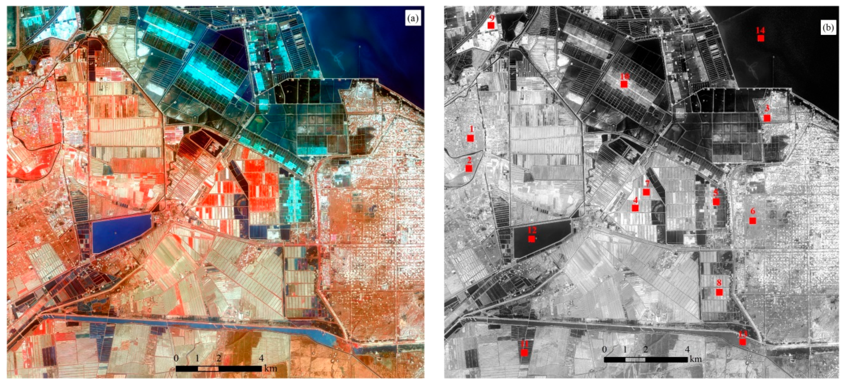
2.1. Study Area and Data
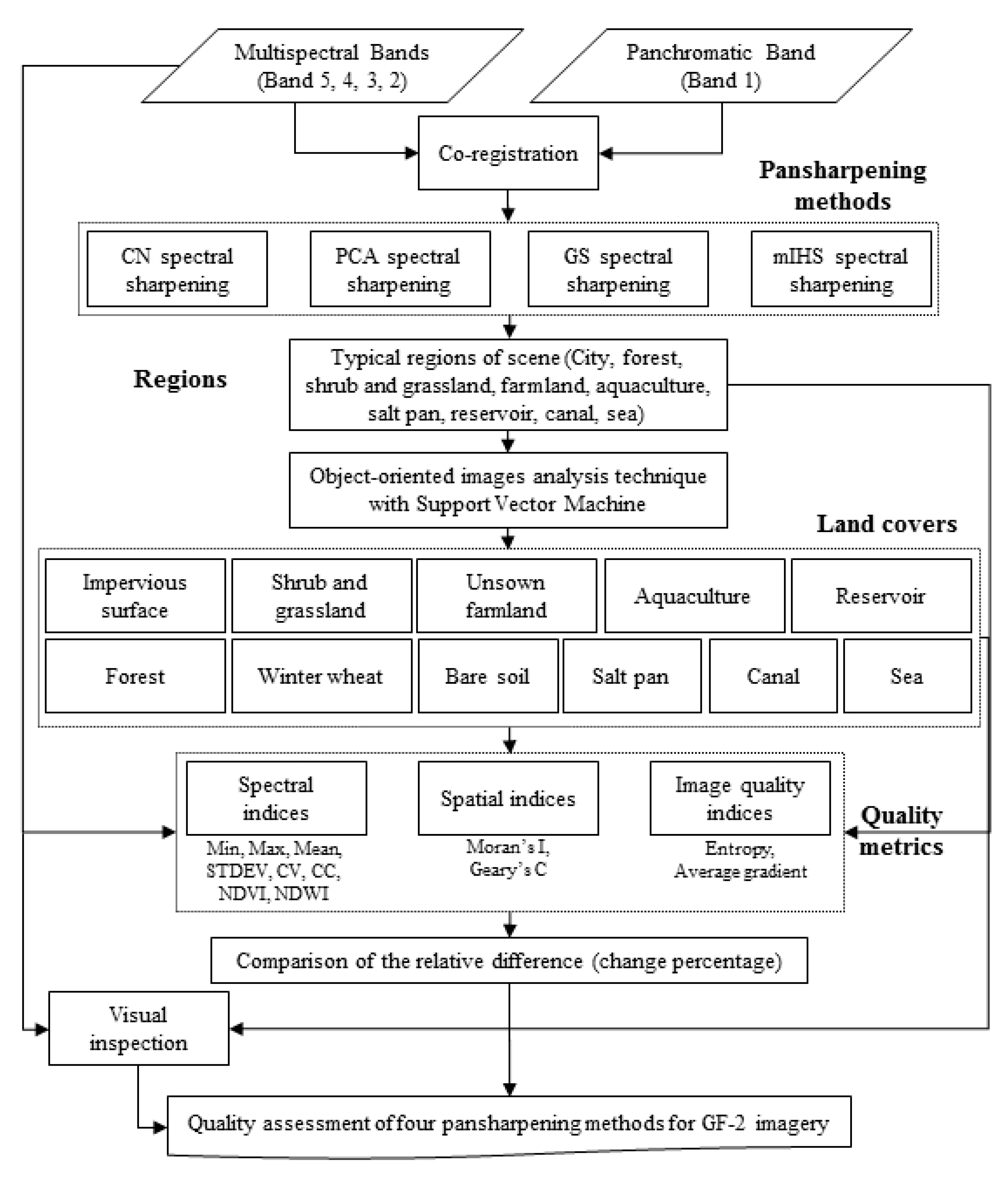
A cloudless GF-2 image downloaded from the China Center for Resources Satellite Data and Application (CRESDA, http://www.cresda.com) was used for a quality assessment of the pansharpened image. The image, which was acquired on 30 April 2016 over the city of Dongying, Shandong Province, China, includes various types of land cover, such as impervious areas, a Robinia pseudoacacia plantation, shrubs and grasslands, winter wheat fields, unsown farmlands, bare soil, salt pans, aquaculture areas, rivers and canals, reservoirs, and the sea. Due to the flat terrain and the difficulty in obtaining fine resolution digital elevation model data for the research area, topographic correction was not used in this study. The PAN and MS images are displayed in Figure 1.
Performing a quantitative quality assessment on the whole pansharpened image is time-consuming, and the redundant regions and the complementary or conflicting regions in the images often make the results of the quantitative assessment inconsistent with those of the visual analysis [28]. Moreover, some pansharpening approaches, such as the Ehlers spatial enhancement method embedded in the ERDAS Imagine Software, require large amounts of storage space and computer memory. Thus, quantitative assessments are often performed for some regions such as urban regions, rural regions, and vegetated regions, and pansharpened images are easier to display in the visualization mode. In this study, 14 regions (showed as the red square areas (400 × 400 pixels) in Figure 1) were selected for the quantitative assessment: Region 1 (urban region (the red square area labeled 1 in Figure 1b), shown in Figure 2); Region 2 (forest region, shown in Figure A1 from Appendix A); Regions 3 and 6 (shrub and grassland regions, Region 3 shown in Figure A2 from Appendix A); Regions 4, 7, and 8 (farmland regions, Regions shown in Figure A3 from Appendix A); Regions 5, 9, and 10 (salt pan regions, Region 5 shown in Figure A4 from Appendix A), Region 11 (aquaculture region), Region 12 (reservoir area), Region 13 (canal area), and Region 14 (sea area). The quantitative assessments for the regions may be disturbed owing to the different proportions of land covers in the regions, because major differences in a land cover can be minimized by small differences in another land cover [15]. Therefore, we further analyzed the quality of the pansharpened images with regard to 11 types of land cover such as impervious surface, forest, shrub and grassland, bare soil, winter wheat, unsown farmland, canal area, salt water in the salt pan, aquaculture water, reservoir water, and sea water. The land-cover percentages for each region are presented in Table 2.

2.2. Method

In the present study, four pansharpening approaches (CN, PCA, GS, and mIHS) were used for sharpening the GF-2 image. The CN spectral sharpening method is an extension of the color normalization algorithm, which uses the PAN band to enhance the MS bands and can be used to simultaneously sharpen any number of bands and maintain the data type and dynamic range of the original image. The PCA spectral sharpening method applies the principal component transformation to convert the MS bands into principal components, and then an inverse principal component transformation is performed on the principal components, where the first principal component is displaced by the matched PAN band. The GS spectral method has a similar procedure to the PCA spectral sharpening method. The difference is that the first component of the GS transformation is replaced by the adjusted PAN band. Compared with the PCA method, the GS method is more accurate because it uses the spectral response function of a given sensor to simulate the PAN band. In this study, the average of the MS bands was used to simulate the low-spatial resolution PAN band. The mIHS sharpening method is an extension of the intensity-hue-saturation transformation and can sharpen four MS bands by iteratively repeating the sharpened process, each for three different MS bands. In this study, two iterations using red/green/blue and near-infrared (NIR)/red/green bands were selected to produce a sharpened image with all four bands. Additional details regarding these pansharpening approaches can be found in the literature [8,9,10,11,12,13,33], and the procedures are described in the ENVI v5.1 (Boulder, CO, USA) software (for the CN, PCA, and GS spectral sharpening methods) and ERDAS imagine v9.2 (Madison, AL, USA) software (for the mIHS method) manuals.
A visual analysis of the pansharpened images, i.e., the conventional method, is necessary [1,34,35,36], as the results and method ranking from the quantitative evaluation were typically inconsistent with those of remote-sensing experts [36]. Moreover, until now, no promising quantitative indices have been reported for the effective assessment of pansharpened images [2]. Although no standardization or universal adoption of the visual evaluation process has been devised until now [22], qualitative quality assessment is often performed according to the different band false-color combinations associated with color preservation and spectral consistency [34].
This is typically time-consuming and expensive, depends significantly on the experience of the interpreter, and cannot yet be automated by a computer system [16,17,28,34,35,37]. Therefore, quantitative quality assessment is usually employed for measuring the spectral and spatial fidelity of pansharpened images [16,35]. Several quantitative quality assessment indices have been reported. Thomas and Wald (2006) divided 39 different indices into seven categories according to a mathematical analysis [18], and Ma et al. (2016) categorized the existing quantitative quality assessment indices into three types [27]. In general, these indices should be objective, reproducible, and of a quantitative nature [34]. Because the quantitative analysis was checked on the native level of the images in this study, the following indices were selected to directly evaluate the spectral and spatial fidelity of the pansharpened images compared with the original MS images: 1) spectral assessment—the minimum (Min), maximum (Max), mean, the STDEV, coefficient of variance (CV), correlation coefficient (CC) between the four bands (the blue (B), green (G), red (R), and near-infrared band (NIR)), normalized difference vegetation index (NDVI, (NIR − Red)/(NIR + Red)), and normalized difference water index (NDWI, (Green − NIR)/(Green + NIR)) were used, which emphasize the spectral preservation; 2) spatial evaluation—the global spatial statistical indices such as the Moran’s I (MoranI) and Geary’s C (GearyC) were applied, which measure the spatial information; and 3) image quality—the EN and AG indices were used, which emphasize the quality of the pansharpened images. The NDVI is sensitive to green vegetation even for areas with low vegetation cover and was first used in 1973 by Rouse et al. [38]. The NDWI is sensitive to water features and eliminates the effects of soil and vegetation features [39]. Both indices have been widely used for studying global vegetation dynamics and monitoring plant canopy and soil moisture. In this study, the differences in the NDVI and NDWI between the pansharpened and original MS images were considered as the spectral quality indices. The MoranI index measures the local homogeneity by comparing the differences between neighboring pixels and the mean. The value range is +1 to −1; +1, 0, and −1 represent strong positive spatial autocorrelation, spatially uncorrelated data, and strong negative spatial autocorrelation, respectively. The GearyC index provides a measure of the dissimilarity within a dataset by comparing the differences between neighboring pixels and the standard deviation. The value range is 0 to 2; 0, 1, and 2 represent strong positive spatial autocorrelation, spatially uncorrelated data, and strong negative spatial autocorrelation, respectively. The EN surveys the amount of information in a pansharpened image. A larger EN corresponds to better performance of the pansharpening method but possibly a larger amount of noise in the pansharpened image. Thus, the EN is often used as a supplemental index [19,40]. The AG measures the detail and texture of a pansharpened image. A larger AG corresponds to better performance of a given pansharpening method [19]. With the exception of the EN and AG indices, which were programmed in the IDL v8.2 software (Boulder, CO, USA), the other 10 indices were calculated in the ENVI v5.1 software. The mathematical expression and the ideal values were in accordance with previous studies [8,9,10,11,12,13,33] and the ENVI v5.1 software manual. The quality assessment was justified by the relative difference (change percentage = (the difference between the metric value of the original and pansharpened MS image/the metric value of the original MS image) × 100%) between the metric values of the original MS image and the pansharpened data, rather than a statistical comparison, because only one scene of the GF-2 image was used. However, some studies indicated that it is necessary to perform a statistical comparison for image pansharpening research [41,42].
For analyzing the effects of the pansharpening methods on different land covers, the first step was to segment the pansharpened and original MS images. Because the pansharpened images had more details than the original MS images, the segmentation results for the GS pansharpened images were used for 11 regions. Region 12 (reservoir region), Region 13 (canal region), and Region 14 (sea region) had only one type of land cover; thus, segmentation was not performed. The segmentation and classification processes were described in our previous work [43], which indicated that this approach provided high classification accuracy with GF-2 imagery. The approach involved identifying the objects via an object-oriented image analysis technique based on the edge algorithm at the scale level (50) and merge level (90) which were determined by repeated experiments. Then, the obtained segments were classified via a support vector machine-supervised method. In order to facilitate comparison with previous research results, and reveal the difference of pansharpened quality over regions and land covers, quality assessment was carried out by regions and land covers. Figure 3 shows a flowchart of this study.

3. Results

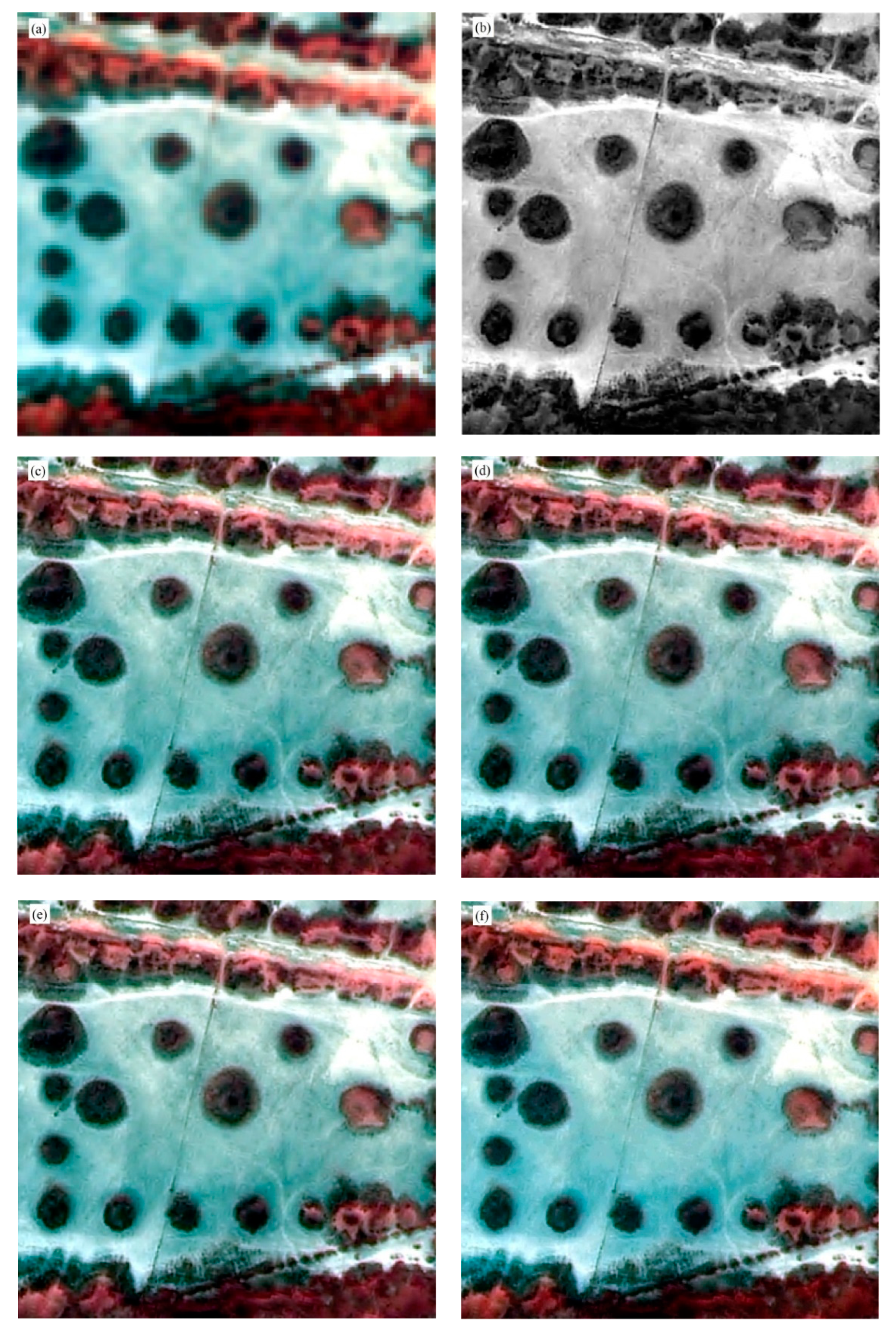
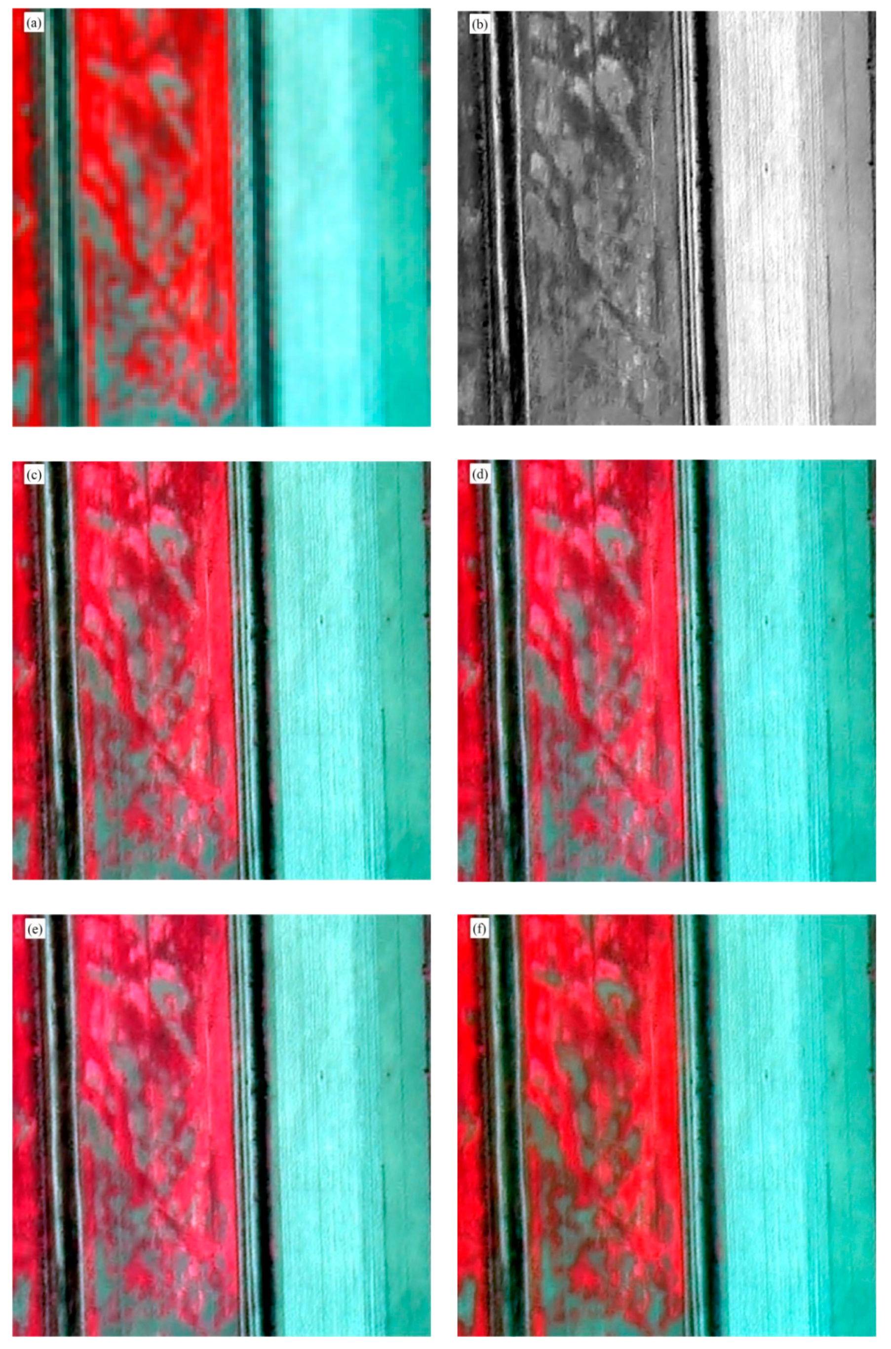
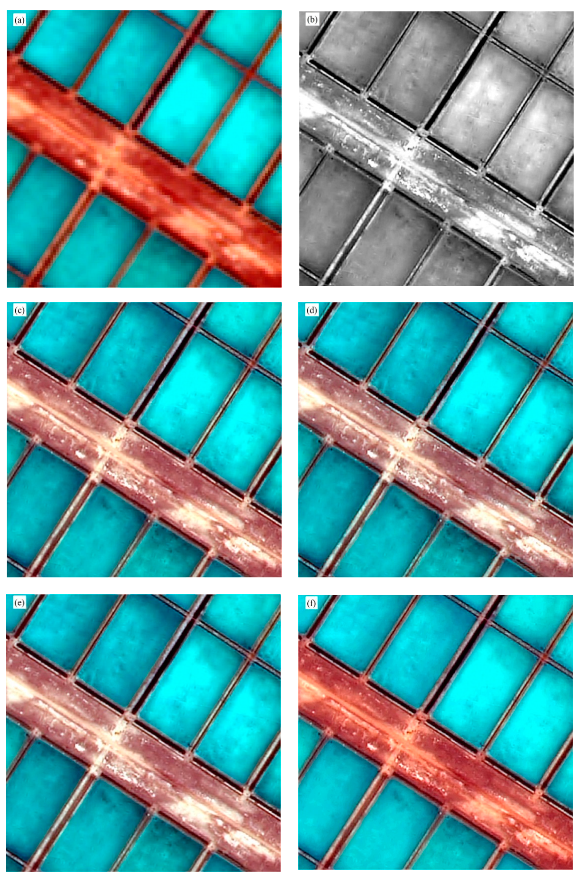
3.1. Visual Analysis

Compared with the original MS image, the pansharpened images exhibit an obvious improvement in spatial quality shown in Figure 2, and Figure A1 to Figure A4 from Appendix A. The original MS images were shown in Figure 2a, Figure A1a, Figure A2a, Figure A3a, and Figure A4a, and the original PAN images were Figure 2b, Figure A1b, Figure A2b, Figure A3b, and Figure A4b. Slight variations are observed between the pansharpened images (Figure 2c to Figure 2f, Figure A1c to Figure A1f, Figure A2c to Figure A2f, Figure A3c to Figure A3f, and Figure A4c to Figure A4f), but in general, all the approaches satisfy the criteria for improving the spatial resolution of the original MS image. A visual evaluation of the spectral quality was performed using the false-color image. When the spectral information is preserved perfectly, the land covers in the pansharpened images have a similar tone to those in the original MS images. Comparing the images resulting from the different pansharpening methods revealed that the pansharpened images had color distortions, as evidenced by the tone changes of the land covers in these images. In the cases of the forest region (Figure A1), and shrub and grassland region (Figure A2), it was difficult to visually detect color differences among the pansharpened images (Figure A1c to Figure A1f, and Figure A2c to Figure A2f). Figure 2, Figure A3 and Figure A4 showed that, visually, the best color-preserving results were obtained with the mIHS pansharpening method, particularly for trees in the urban region (Figure 2f), winter wheat (Figure A3f), bare salt-affected soil and salt water (Figure A4f). The PCA pansharpening method exhibited the worst color-preserving results (Figure 2e, Figure A3e, and Figure A4e).

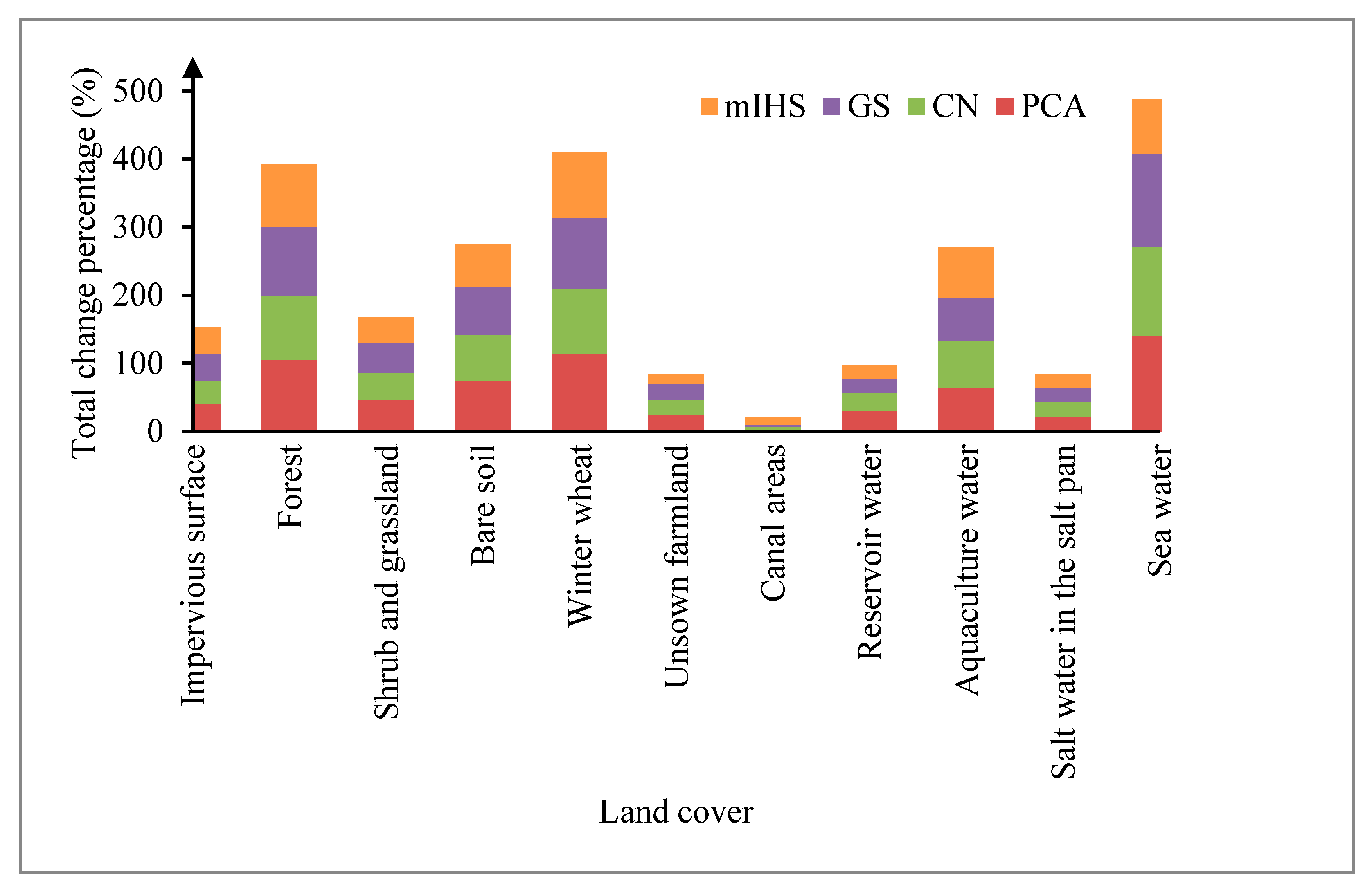
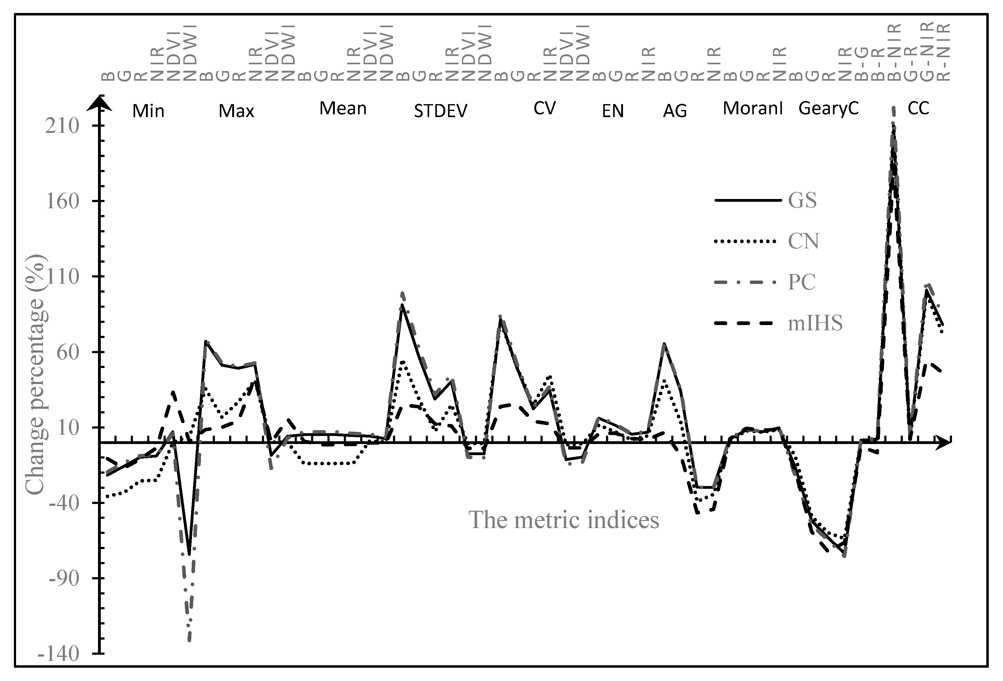
3.2. Quantitative Quality Assessment by Region

In this study, 14 regions were employed for the quantitative assessment. Owing to length limitations, only quality assessment results of the urban region (Region 1) are displayed in Figure 4.
All four pansharpening methods reduced the Min values of the employed regions compared with the original MS bands (see Figure 4), with only one exception: the farmland (Region 4), for which the PCA method increased the Min values of the blue, green, and red band, and the GS method increased the Min value of the red band. In contrast to the Min values, the GS, PCA, and mIHS pansharpening methods increased the Max values in all four bands of the regions compared with the original MS bands (see Figure 4). The CN method reduced the Max values in all four bands of the regions compared with the original MS bands, with only one exception (the urban region, i.e., Region 1, shown in Figure 4). This means that the pansharpening expands the range of spectral values of four bands. In general, the four pansharpening methods changed the Min value less than the Max value of the regions. The CN method obtained the biggest difference in Min values of all four bands in the urban, forest, shrub and grassland, farmland, and salt pan regions, and the PCA method obtained the biggest difference in Max value of the regions. The mIHS method exhibited the smallest difference in the Min NDVI values in the forest (0.3%), shrub and grassland (0.1%), and farmland region (−0.3%), and the smallest difference in the Max NDVI values in the forest (−10.6%), shrub and grassland (−0.5%), and farmland (−0.2%) regions, followed by the CN, GS, and PCA method. For the NDWI, the CN and mIHS methods exhibited the smaller difference in the Min and Max values compared with the original NDWI values.
For the Mean value, compared with the GS, CN, and PCA methods, the mIHS pansharpening method exhibited the smallest difference for all four bands in all regions, followed by the GS, PCA, and the CN method (see Figure 4). Compared with the mIHS and CN methods, the GS and PCA methods produced the bigger difference in the Mean NDVI value in the forest, and farmland regions, which indicated that the NDVI values from the GS and PCA pansharpened images should be calibrated before use. For the STDEV value, the mIHS pansharpening method exhibited the smallest difference for all four bans for the regions (see Figure 4), with one exception: the farmland region. For the CV value, the mIHS pansharpening method exhibited the smallest difference for all four bands in all regions (see Figure 4), with one exception: the farmland region. For preserving the CV value of all four bands, the mIHS method was best, followed by the GS, CN, and the PCA method. However, for preserving the CV values in NDVI and NDWI indices, the CN method was best in the shrub and grassland, farmland, and urban regions, followed by the mIHS, GS, and the PCA method.
For the EN, the mIHS method exhibited the smallest difference in the NIR band for all regions (−0.9% in salt pan region), the smallest difference in the blue band for the city, forest, shrub and grassland, and farmland regions (−1.8% in farmland region), the smallest difference in the green band for the urban, forest, shrub and grassland, and salt pan regions (0.3% in salt pan region), and the smallest difference in the red band for the forest, shrub and grassland, and salt pan regions (0.0% in shrub and grassland region). For preserving the EN value of all four bands, the mIHS method was best, followed by the CN method (see Figure 4). The PCA method was worst. In general, the change of EN values of the shrub and grassland, farmland, and salt pan regions by all pansharpening methods was less than that of the urban, and forest regions. For preserving the AG value (see Figure 4), the GS method was best, followed by the mIHS method. The PCA method was worst.
For the spatial indices (MoranI and GearyC), the CN method was best for urban, shrub and grassland, and farmland regions, followed by the mIHS method. In general, the change of MoranI values of shrub and grassland, farmland, and salt pan regions by all pansharpening methods was less than that of urban, and forest regions. For preserving the Moran I and GearyC indices (see Figure 4), the CN method was best, followed by the mIHS method. The GS method was worst.
For preserving the CC values between the four bands, the mIHS method was best, followed by the CN method (see Figure 4). The PCA method was worst. In general, the change of CC values of shrub and grassland, and forest regions by all pansharpening methods was less than that of urban, salt pan, and farmland regions.
The foregoing quantitative assessment results were consistent with the results of the visual analysis; i.e., the mIHS method exhibited the best performance. However, the quantitative assessment captured statistical features that the visual analysis could not perceive because of a weak color difference among the pansharpened images. The results indicated that the mIHS method was the best for maintaining the spectral information of the pansharpened images, and the CN method was the best for maintaining the spatial information of the pansharpened images.

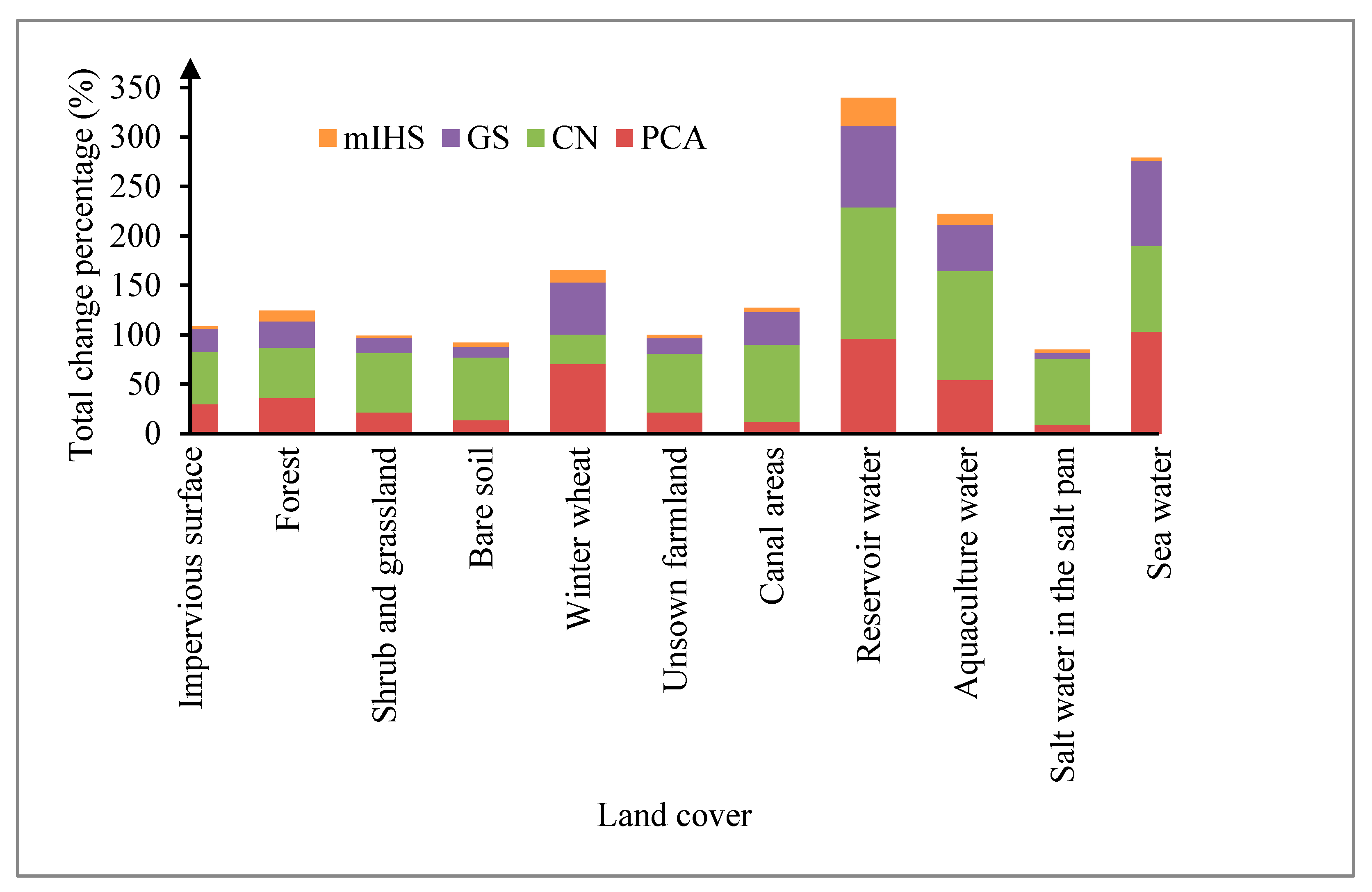
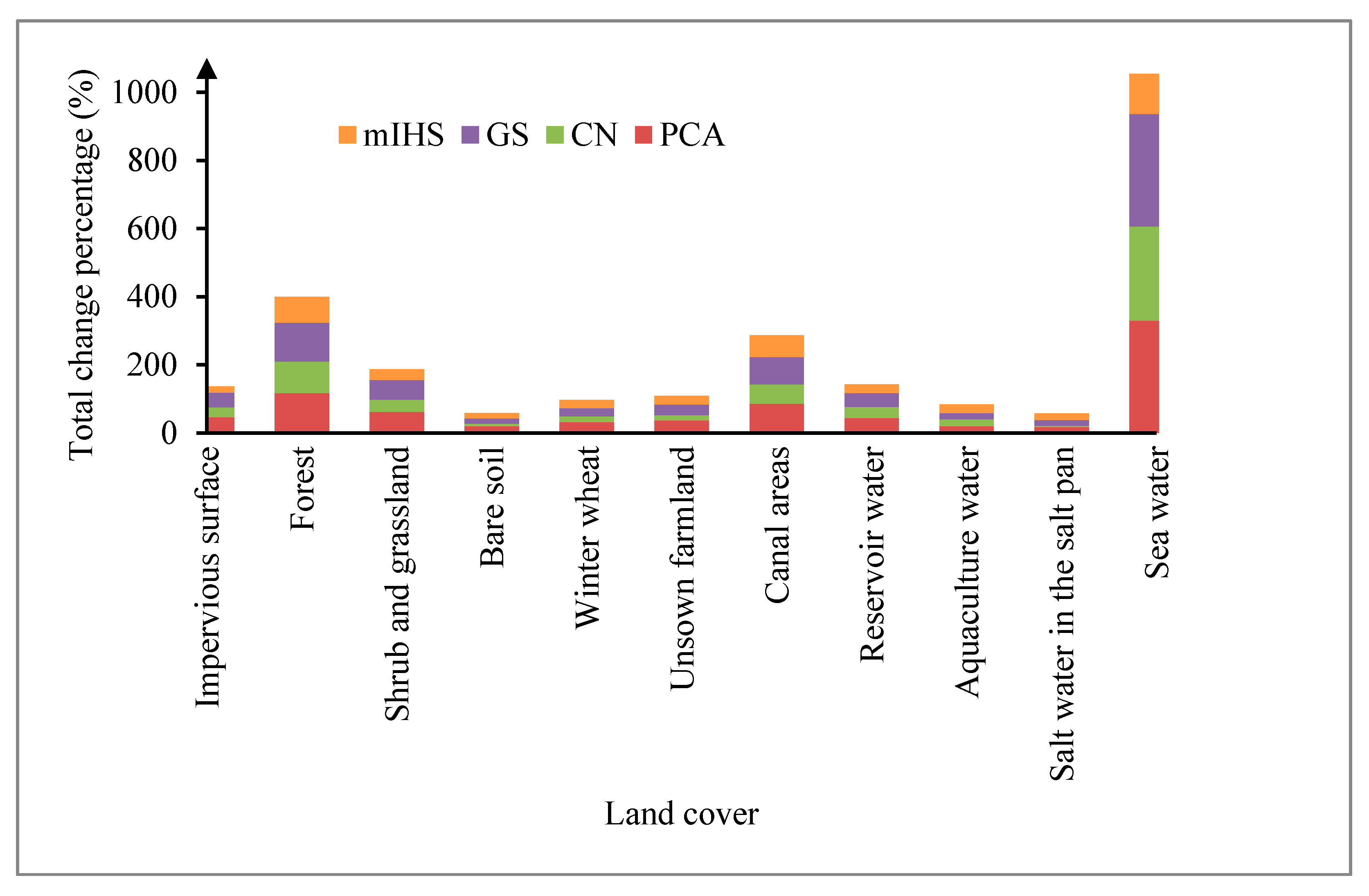
3.3. Quantitative Quality Assessment by Land Covers

The segmented image and land covers from the GS pansharpened images are shown in Figure 5. The quality indices were applied only to pixels associated with a certain land cover. To evaluate the degree of quality-index preservation, the sum of the absolute change values of the quality index was calculated. A smaller sum indicated a better capability of the pansharpening method to preserve the quality index. The following analysis focuses on comparisons of the Mean, EN, MoranI, and CC values between the pansharpened images.
For preserving the Mean values (spectral analysis) of the original MS image (with regard to the percentage change), the mIHS method achieved the best result for the shrub and grassland (the sum of all four band variations was 2.0%), followed by the impervious surfaces (2.2%), sea water (2.9%), unsown farmland (3.4%), salt water in the salt pan (3.7%), bare soil (4.1%), canal areas (4.2%), aquaculture water (10.7%), forest (11.1%), winter wheat (12.6%), and reservoir water (28.6%). The PCA method achieved the best result for the salt water in the salt pan (8.8%), followed by the canal area (11.8%), bare soil (13.6%), unsown farmland (21.5%), shrub and grassland (21.6%), impervious surface (29.9%), forest (35.9%), aquaculture water (54.4%), winter wheat (70.4%), reservoir water (96.4%), and sea water (103.2%). The CN method achieved the best result for the winter wheat (30.1%), followed by the forest (51.1%), impervious surface (52.7%), unsown farmland (59.2%), shrub and grassland (60.0%), bare soil (63.6%), salt water in the salt pan (66.8%), canal area (78.3%), sea water (87.0%), aquaculture water (110.1%), and reservoir water (132.8%). The GS method exhibited the best result for the salt water in the salt pan (5.9%), followed by the bare soil (10.7%), shrub and grassland (15.5%), unsown farmland (15.9%), impervious surface (23.7%), forest (26.5%), canal areas (33.0%), aquaculture water (47.1%), winter wheat (52.4%), reservoir water (81.7%), and sea water (85.9%). Therefore, with regard to the Mean values (spectral analysis), the mIHS was typically the best pansharpening method for all land covers, followed by the GS, PCA, and CN methods (see Figure A5 from Appendix B).
For preserving the EN values, the mIHS method achieved the best result for the bare soil (the sum of all four band variations was 14.9%), followed by the impervious surface (18.3%), salt water in the salt pan (19.8%), winter wheat (24.1%), reservoir water (25.1%), aquaculture water (26.0%), unsown farmland (26.3%), shrub and grassland (31.2%), canal area (62.8%), forest (74.9%), and sea water (118.6%). The PCA method achieved the best result for the salt water in the salt pan (18.4%), followed by the aquaculture water (20.6%), bare soil (20.9%), winter wheat (32.6%), unsown farmland (37.0%), reservoir water (44.3%), impervious surface (46.8%), shrub and grassland (62.0%), canal areas (87.2%), forest (117.8%), and sea water (330.2%). The CN method achieved the best result for the salt water in the salt pan (3.4%), followed by the bare soil (6.4%), unsown farmland (16.1%), winter wheat (16.9%), aquaculture water (20.0%), impervious surface (28.6%), reservoir water (32.4%), shrub and grassland (36.3%), canal areas (56.4%), forest (92.4%), and sea water (275.9%). The GS method achieved the best result for the bare soil (16.4%), followed by the salt water in the salt pan (16.5%), aquaculture water (18.1%), winter wheat (24.1%), unsown farmland (30.6%), reservoir water (41.2%), impervious surface (43.7%), shrub and grassland (57.9%), canal areas (80.0%), forest (114.0%), and sea water (330.3%). Therefore, with regard to preserving the EN values, for impervious surface, forest, shrub and grassland, reservoir water, and sea water, the mIHS method can achieve the best pansharpened result, and for bare soil, winter wheat, unsown farmland, canal area, and salt water in the salt pan, the CN method can achieve the best pansharpened result, and for aquaculture water, the GS method can achieve the best pansharpened result (see Figure A6 from Appendix B). Because these results could be affected by noise, they should be interpreted with caution.
For preserving (with regard to the percentage change) the MoranI values (global spatial analysis) of the original MS image, the mIHS method achieved the best result for the canal areas (the sum of all four band variations was 11.0%), followed by the unsown farmland (15.4%), reservoir water (19.2%), salt water in the salt pan (19.8%), shrub and grassland (38.6%), impervious surface (38.9%), bare soil (62.3%), aquaculture water (74.3%), sea water (80.7%), forest (92.2%), and winter wheat (95.0%). The PCA method achieved the best result for the canal areas (the sum of all four band variations was 2.4%), followed by the salt water in the salt pan (22.2%), unsown farmland (24.8%), reservoir water (29.7%), impervious surface (40.3%), shrub and grassland (46.7%), aquaculture water (63.9%), bare soil (73.9%), forest (104.8%), winter wheat (113.3%), and sea water (139.9%). The CN method achieved the best result for the canal areas (the sum of all four band variations was 3.9%), followed by the salt water in the salt pan (20.6%), the unsown farmland (21.5%), reservoir water (26.9%), impervious surface (34.8%), shrub and grassland (39.1%), bare soil (67.8%), aquaculture water (68.4%), forest (94.7%), winter wheat (96.0%), and sea water (131.2%). The GS method achieved the best result for the canal areas (the sum of all four band variations was 2.8%), followed by the reservoir water (20.4%), salt water in the salt pan (21.6%), unsown farmland (23.0%), impervious surface (38.3%), shrub and grassland (43.5%), aquaculture water (63.2%), bare soil (70.9%), forest (100.5%), winter wheat (104.9%), and sea water (136.9%). Therefore, with regard to the MoranI and GearyI values, for impervious surface, the CN method can achieve the best pansharpened result, and for forest, shrub and grassland, bare soil, winter wheat, unsown farmland, reservoir water, sea water, and salt water in the salt pan, the mIHS method can achieve the best pansharpened result, and for canal area, the PCA method can achieve the best pansharpened result, and for aquaculture water, the GS method can achieve the best pansharpened result (see Figure A7 from Appendix B).
For preserving the CC values between the four bands, for unsown farmland, the four pansharpening methods exhibited similar potential. The mIHS method achieved the best result for the salt water in the salt pan (the sum of the variation of the six CC values was 3.6%), followed by the unsown farmland (12.8%), bare soil (28.7%), impervious surface (128.6%), shrub and grassland (155.2%), reservoir water (207.7%), aquaculture water (220.7%), winter wheat (316.1%), canal areas (537,1%), sea water (583.1%), and forest (868.6%). The PCA method achieved the best result for the unsown farmland (12.4%), followed by the salt water in the salt pan (25.8%), bare soil (101.9%), aquaculture water (120.4%), reservoir water (189.1%), impervious surface (198.1%), shrub and grassland (216.8%), winter wheat (577.0%), canal areas (642.2%), sea water (881.3%), and forest (1022.1%). The CN method achieved the best result for the unsown farmland (11.2%), followed by the salt water in the salt pan (21.1%), bare soil (88.7%), aquaculture water (105.7%), impervious surface (177.9%), reservoir water (204.0%), shrub and grassland (204.5%), winter wheat (425.9%), canal areas (621.9%), sea water (839.8%), and forest (990.2%). The GS method achieved the best result for the unsown farmland (11.7%), followed by the salt water in the salt pan (21.9%), aquaculture water (84.3%), bare soil (89.1%), impervious surface (187.6%), shrub and grassland (193.5%), reservoir water (204.0%), winter wheat (504.6%), canal areas (598.7%), sea water (878.9%), and forest (979.1%). Generally, reducing the CC value between bands was helpful for reducing the amount of redundant information between the bands, although it could change the relationship between them, thereby affecting various indices, such as the NDVI and NDWI. Therefore, with regard to preserving the CC values between the four bands, for impervious surface, forest, shrub and grassland, bare soil, winter wheat, canal area, sea water, and salt water in the salt pan, the mIHS method can achieve the best pansharpened result, and for unsown farmland, the CN method can achieve the best pansharpened result, and for reservoir water, the PCA method can achieve the best pansharpened result, for aquaculture water, the GS method can achieve the best pansharpened result (see Figure A8 from Appendix B). Generally, for most land covers, the mIHS method was the best, and the PCA method was the worst.

4. Discussion

The quality of the pansharpened image was inconsistent among the different regions and different land covers; thus, most of the quantitative quality assessment strategies that involve assigning a single value to the whole image could not efficiently evaluate the effectiveness of the pansharpening methods [44]. An object-level or land-cover-based pansharpening quality assessment strategy could overcome the limitations of the traditional quantitative quality assessment strategies, evaluate the performance of the pansharpening process for different land covers, and quantify the quality of different land covers, thus improving our understanding of the influence of pansharpening methods across different land covers [15,44]. However, relevant research has only focused on a few types of land covers [15,44], and it is necessary to evaluate the performance of the pansharpening process for more land covers. The objective of the present study was to elucidate the effects of commonly used pansharpening methods when they are applied to GF-2 imagery by performing quality assessments based on the region and land cover. The GS, CN, PCA, and mIHS pansharpening techniques were applied and evaluated using a series of quality metrics.
Visual inspections were performed only for the regions composed of different proportions of the different land covers. Generally, all four approaches satisfied the requirements for improving the spatial resolution of the original MS image. The mIHS pansharpening method produced better results than the GS, CN, and PCA pansharpening methods. The previous studies also indicated that the colors of PCA pansharpened images were lighter than those of the original MS images [27,45]. It was difficult to compare the color fidelity of the GS and CN methods through visual analysis. Our results are consistent with those of Nikolakopoulos and Oikonomidis (2015) and Su et al. (2012) and partly consistent with those of Witharana et al. (2013) and Vivone et al. (2015) [12,32,37,46], who reported that the behavior of the pansharpening method was related to the context of the images. However, our results are inconsistent with those of Yuhendra et al., who reported that the false-color composite of the GS pansharpened WorldView-2 bands 3 (green band), 5 (red band), and 7 (blue) was closer to the colors in the original low-resolution MS image than that of an mIHS pansharpened image [47]. Our results are consistent with those of Kang et al., who reported that a mIHS pansharpened image had little change in the colors of water and rock, whereas the color distortion for a PCA pansharpened image was significant [48]. The previous studies indicated that the mIHS, GS, CN, and PCA pansharpening methods performed well for some images but not for others [31,49]. In fact, visual analysis was not sufficient to evaluate the quality of the pansharpening methods; the results should always be confirmed via quantitative quality assessment [12,37].

4.1. Impact of Pansharpening Methods in Different Regions and Imagries Acquired with Various Satellites

Generally, the preservation of the statistical parameters of the image was necessary when the scholars wished to calculate the vegetation indices and perform classification according to the spectral-curve similarity among land covers [45]. Regarding spectral analysis (Min, Max, Mean, STDEV, CV, CC, NDVI, NDWI), the mIHS method resulted in minor changes to the statistical indices compared with the CN, GS, and PCA methods. However, for the vegetation-dominated regions, the PCA method resulted in minor changes to the Min values in the green and red bands for the forest area; in the blue, green, and NIR bands for the farmland area; and in the green, red, and NIR bands for the shrub and grassland area. For the vegetation-dominated and salt pan regions, the CN pansharpening method resulted in minor changes to the Max values in the blue and NIR bands and the NDVI for forest area; the blue and NIR bands for the farmland area; the blue, green, red, and NIR bands for the shrub and grassland area; and the blue band and the NDVI for the salt pan area. Except for an increase in the Min value in the red band for the GS pansharpening method and in the blue, green, and red bands for the PCA pansharpening method in the winter wheat and farmland area (Region 4), all four pansharpening methods reduced the Min values of all four bands, and the mIHS, GS, and PCA methods increased the Max values of all four bands in Regions 1–5. This is partly consistent with the results reported by Nikolakopoulos (2008) for the effects of the PCA and mIHS methods on the Min and Max values [45]. Regarding only urban areas, the results of this study differed from those of Nikolakopoulos (2008), who reported that the mIHS method reduced the correlation values of all the bands of a QuickBird urban image, and the PCA method increased them [45]. Overall, the foregoing results for the spectral indices indicate the superiority of the mIHS pansharpening method to the GS, CN, and PCA methods. This is consistent with the results of previous studies [7,12], as well as previous results for the GS and PCA pansharpening methods [23,30,32,36,46,50,51]. It is also consistent with previous results for the mIHS and PCA pansharpening methods [48,52] and the mIHS, GS, and PCA pansharpening methods [53]. However, it is inconsistent with the findings of Sarp, who reported that the PCA method produced better results than the GS pansharpening method for the difference in the correlation coefficient and root mean square error (RMSE) values between the images before and after fusion in both IKONOS and QuickBird in Istanbul [30]. Additionally, it is inconsistent with the result of Jawak and Luis, who reported that the GS pansharpening method performed better for WorldView-2 images than the mIHS method with regard to the mean bias, median bias, mode bias, RMSE, and structure similarity index (SSIM) [54]. Sometimes, the quality assessment results for the different quality indices were contradictory; for example, the PC pansharpened IKONOS and QuickBird images were evaluated as the worst according to the spectral angle mapper index but the best according to the RMSE index, and overall, they were evaluated as the worst via a mean opinion score test [55]. The results of pansharpening the SPOT 4 or SPOT 5 MS images with the PAN IKONOS image indicated that the best results were achieved by the CN method, followed by the GS and PCA methods, with regard to the correlation coefficient index (CCI), deviation per pixel index, and SSIM and the GS, PCA, and CN methods with regard to the RMSE [34]. For a WorldView-2 image, the GS method was worse than the mIHS method with regard to the CCI and SSIM, whereas it was better than the mIHS method with regard to the RMSE and signal-to-noise ratio [47].
With regard to preserving the MoranI and GearyI values (global spatial analysis), the best result for urban regions was achieved by the CN method, followed by the GS, mIHS, and PCA methods. For forest region, the best result was achieved by the PCA pansharpening method. The CN method exhibited the best performance for shrub and grassland regions, farmland regions, and salt pan regions. For aquaculture, and sea regions, the best result was achieved by the mIHS method. The GS method was the most effective for reservoir, and canal regions. These results are consistent with those of Witharana et al., who reported that for GeoEye-1 urban images, the CN method exhibited the highest scores for spatial metrics, followed by the mIHS, GS, and PCA methods, although different spatial metrics, such as the canny edge detection filter, the high-pass correlation coefficient, and the RMSE of a Sobel-filtered edge image, were used [37]. The results are also consistent with previous studies in which the mIHS method achieved better scores for spatial information than the PC method [32,52].
Regarding the EN and AG values (image quality analysis), for urban regions, the mIHS method resulted in the smallest changes to the EN and AG values, followed by the PCA, CN, and GS pansharpening methods. This is partly consistent with previous results indicating that the mIHS method resulted in the smallest changes to the EN values, followed by the GS, PCA, and CN methods, for the town of Killinochchi, Sri Lanka, and for the city of Rome, Italy [12]. The inconsistency may be due to the imagery from different sensors and urban regions composed of different land covers. With regard to the increasing EN and AG values, the PCA method was superior to the mIHS method, which is consistent with the results of Kang et al. (2008) [48]. Generally, a larger EN value corresponds to a larger amount of information in the image, and a larger AG value corresponds to higher clarity of the image. However, these values are affected by the noise in a pansharpened image. Therefore, the results for the increase in the EN and AG values should be interpreted with caution.
Overall, the quantitative assessment by regions demonstrated that independent of regions, the mIHS method produced better results than the GS, PCA, and the CN method by preserving the colors of the original MS image. The mIHS, GS, and PC methods produced all the smallest spectral variations in the shrub and grassland region, and the CN method produced the smallest spectral variations in the farmland region, which indicated that the different pansharpening methods had different effects in the different regions.

4.2. Impact of Pansharpening Methods in Different Land Covers

According to the results of the foregoing assessment based on regions, the behaviors of the pansharpening methods differed among the regions. The main reason for this may be that the different regions had varying proportions of land covers. Thus, it was necessary to analyze the effects of pansharpening methods in the different land covers. In cases where land cover accounted for >50% of a given region, the mIHS method resulted in minor changes to the Mean and STDEV values, and the CN and PCA methods resulted in major changes to them. In cases where shrub and grassland, bare soil, and canals accounted for only small areas in a given region, the behavior of the four pansharpening methods changed and sometimes exhibited contrary results. Additional experiments must be performed for more regions to further investigate this. The impervious surface of Region 1 had higher STDEV values in the original MS image than that of Region 2. The mIHS, GS, and PCA methods resulted in minor changes to the Mean value and major changes to the STDEV value for the impervious surface from Region 1 compared with the impervious surface from Region 2. This indicates that the higher values of the STDEV of the impervious surface in the original MS images resulted in higher-quality pansharpened images, which is consistent with the results of DadrasJavan and Samadzadegan (2014) [44]. However, the CN method produced opposite results. For the forest, Region 1 had higher STDEV values than Region 2 for all four bands in the original MS image. Only the GS and PCA methods resulted in minor changes to the Mean value for Region 1, and the mIHS and CN methods produced opposite results. All four pansharpening methods resulted in major changes to the STDEV values for Region 2 compared with those of Region 1. Compared with the impervious surface, the forest had smaller STDEV, CV, EN, and AG values, and the mIHS pansharpened image of the forest had the bigger difference in the Mean and STDEV values compared with the original MS bands than that of the impervious surface, which was consistent with the results at region scale. Therefore, the result that higher STDEV values of the land cover in the original MS images resulted in higher-quality pansharpened images was conditional for the pansharpening methods. This indicates differences in the pansharpened-image quality for different land covers [44]. However, in contrast to other land covers, the same number of spectral distortions in the canal and reservoir regions observed in a previous study was not observed in this study [15]. This should be further investigated. Nevertheless, it could be concluded that the proportion of different land-cover types and the change degree of pansharpening methods to different land covers in different regions could be used to roughly explain the impacts of pansharpening methods in different regions.
With regard to preserving the MoranI and GearyI values (global spatial analysis), the mIHS method best preserved the spatial autocorrelation of most land covers, followed by the CN, GS, and PCA methods. However, for the aquaculture in Region 11 and the salt pan in Region 9, the results were the opposite, and for the impervious surface the CN method was the best and the PCA method was the worst. All four pansharpening methods increased the positive spatial autocorrelation of the impervious surface, forest, shrub and grassland, and bare soil in Region 3 and the winter wheat, unsown farmland, canal, and salt pan in Regions 5 and 10, to varying degrees. For preserving the MoranI value (image spatial autocorrelation preservation), all four pansharpening methods achieved the best result for the canal. For all four methods, the spatial autocorrelation of the forest, winter wheat, and sea water was altered by >90.0% after fusion. The reasons for this large increase should be investigated in the future.
Regarding the EN and AG values (image quality analysis), from the viewpoint of increasing the image information and the texture of the pansharpened image, the PCA method added the largest amount of information and detail to the pansharpened images for most land covers, with the exception of the salt pan. The mIHS pansharpening method added the smallest amount of information and detail to the pansharpened images, except for the salt pan (where the CN method added the smallest amount). For all four pansharpening methods, compared with the other land covers, more information and detail were injected into the pansharpened images for the canal, forest, and sea water. The reasons for this large increase should be investigated in the future.
Overall, it is evident that the behavior of the pansharpening methods was different among the regions, indicating differences in the pansharpening quality over different land covers. For most land covers, the mIHS pansharpening method produced better results than the GS, CN, and PCA methods by preserving the colors of the original MS image. This may be due to the different performances of the four pansharpening methods. In this study, the CN and GS methods essentially used the average values of all four bands to simulate the PAN band, which may have increased the correlation of the pansharpened images. The PCA method replaced the first component with the matched PAN band before the inverse principal component transformation, which may have resulted in the loss of spectral information, including from the original image. However, the mIHS method sharpened the four MS bands by iteratively repeating the sharpening process using the different band combinations and the spectral responses of a given sensor, which made the pansharpened images close to the original bands. For all four pansharpening methods, after pansharpening, the spatial autocorrelation of the forest, winter wheat, and sea water changed by >90.0%, and more information and detail were injected into the canal, forest, and sea water areas of the pansharpened images. This requires further study.

5. Conclusions

Most traditional image pansharpening quality assessment approaches have been performed for the whole image or regions such as urban or agricultural areas. However, major differences in a given region or land cover can be minimized by small differences in another region or land cover. Thus, it is necessary to evaluate the performance of the pansharpening process for different land covers and quantify the quality of the process for different land covers. This enhances our understanding of the effects of pansharpening methods for different land covers. Many quality metrics have been used to evaluate the quality of the pansharpened image at the downsampled scale, but the quality of the pansharpened images obtained using the different pansharpening methods depends on the spatial scale and the imaging sensor. Additionally, the performance of the assessment at the downsampled scale may not be the same as that at the full scale. Moreover, when the existing pansharpening methods are used with imagery captured by new satellites, spectral distortion is a significant issue. Hence, quality assessment of the existing pansharpening methods for images captured by new satellites should be performed. In this study, we evaluated the widely used mIHS, GS, CN, and PCA pansharpening methods for GF-2 imagery with regard to land cover, using several reliable quality indices at the native spatial scale without reference.
Both visual and quantitative analysis by region indicated that all four approaches satisfied the demands for improving the spatial resolution of the original GF-2 MS image, and the mIHS pansharpening method produced better results than the GS, CN, and PCA methods by preserving the colors of the original MS image. The mIHS, GS, CN, and PCA methods performed well for some regions, such as urban, and agricultural regions, but not for others, such as forest, and shrub and grassland regions.
The inconsistency in the quality of the pansharpening methods across various land covers was highlighted in this study. With regard to the Mean and STDEV values (spectral analysis), the mIHS method typically performed the best for most land covers, followed by the GS, PCA, and CN methods. With regard to the MoranI and GearyI values (global spatial analysis), the mIHS method best preserved the spatial autocorrelation for most land covers, followed by the CN, GS, and PCA methods. With regard to the EN and AG values (image quality analysis), from the viewpoint of increasing the image information and texture of the pansharpened image, the PC method added the largest amount of information and detail to the pansharpened images for most land covers (with the exception of the salt pan), and the mIHS method added the smallest amount of information and detail to the pansharpened images. For all four pansharpening methods, after pansharpening, the spatial autocorrelation of the forest, winter wheat, and sea water was altered by >90.0%, and more information and detail was injected into the pansharpened images for the canal, forest, and sea water. This needs to be studied further. Overall, the mIHS method is recommended for pansharpening GF-2 imagery.
In this study, the quality of pansharpening methods was evaluated with regard to the land cover, by calculating the quality indices pixel-by-pixel. In the future, assessments should be performed through a statistical comparison of the individual image object of each land cover using more pansharpening approaches with more image-quality metrics across a larger number of regions with fragmented land cover and terrain. Moreover, effects of atmospheric and topographic correction on the pansharpened images should be considered.

Author Contributions

Conceptualization, Q.L.; Data curation, C.H.; funding acquisition, Q.L.; methodology, Q.L. and C.H.; validation, H.L.; writing—original draft, Q.L.; writing—review and editing, Q.L., C.H. and H.L. All authors have read and agreed to the published version of the manuscript.

Funding

This research was jointly financially supported by the National Natural Science Foundation of China (Project Nos. 4151144012, 41671422, 41661144030), the Strategic Priority Research Program of Chinese Academy of Sciences (Project No. XDA20030302), the National Key Research and Development Program of China (Project No. 2016YFC1402701), the Innovation Project of LREIS (Project Nos. 088RA20CYA, 08R8A010YA), and the National Mountain Flood Disaster Investigation Project (Project No. SHZH-IWHR-57).

Acknowledgments

Thanks to China Center of Resources Satellite Data and Application for providing the GF-2 data products.

Conflicts of Interest

The authors declare no conflict of interest.

Appendix A. The Original Multispectral (MS), Panchromatic (PAN), and Pansharpened Images in Several Regions

Figure A1. Image Region 2—Forest area: (a) multispectral image (100 × 100 pixels, false color NIR, red and green composition); (b) panchromatic image (400 × 400 pixels); (c) Gram–Schmidt pansharpened image (400 × 400 pixels); (d) color normalized algorithm pansharpened image (400 × 400 pixels); (e) principal component analysis pansharpened image (400 × 400 pixels); (f) modified intensity-hue-saturation pansharpened image (400 × 400 pixels). The upper left corner of the image is placed at 662792 E and 4198507 N (UTM geographic coordinates, zone 50, WGS-84).
Applsci 10 03673 g0a1
Figure A2. Image Region 3–Shrub and grassland area: (a) multispectral image (100 × 100 pixels, false color NIR, red and green composition); (b) panchromatic image (400 × 400 pixels); (c) Gram–Schmidt pansharpened image (400 × 400 pixels); (d) color normalized algorithm pansharpened image (400 × 400 pixels); (e) principal component analysis pansharpened image (400 × 400 pixels); (f) modified intensity-hue-saturation pansharpened image (400 × 400 pixels). The upper left corner of the image is placed at 677163 E and 4200929 N (UTM geographic coordinates, zone 50, WGS-84).
Applsci 10 03673 g0a2
Figure A3. Image Region 4–Farmland area: (a) multispectral image (100 × 100 pixels, false color NIR, red and green composition); (b) panchromatic image (400 × 400 pixels); (c) Gram–Schmidt pansharpened image (400 × 400 pixels); (d) color normalized algorithm pansharpened image (400 × 400 pixels); (e) principal component analysis pansharpened image (400 × 400 pixels); (f) modified intensity-hue-saturation pansharpened image (400 × 400 pixels). The upper left corner of the image is placed at 670814 E and 4196593 N (UTM geographic coordinates, zone 50, WGS-84).
Applsci 10 03673 g0a3
Figure A4. Image Region 5—Salt pan area: (a) multispectral image (100 × 100 pixels, false color NIR, red and green composition); (b) panchromatic image (400 × 400 pixels); (c) Gram–Schmidt pansharpened image (400 × 400 pixels); (d) color normalized algorithm pansharpened image (400 × 400 pixels); (e) principal component analysis pansharpened image (400 × 400 pixels); (f) modified intensity-hue-saturation pansharpened image (400 × 400 pixels). The upper left corner of the image is placed at 670280 E and 4202564 N (UTM geographic coordinates, zone 50, WGS-84).
Applsci 10 03673 g0a4

Appendix B. Sum of the Relative Differences of Each Quality Metric Index (Mean, Entropy (EN), MoranI, and Correlation Coefficient (CC) Value) of the Blue, Green, Red, and Near Infrared Bands for Each Pansharpening Method

Figure A5. Sum of the relative differences of the mean values of the blue, green, red, and near-infrared bands for the modified intensity-hue-saturation (mIHS), Gram–Schmidt (GS), color normalized algorithm (CN), and principal component analysis (PCA) pansharpening methods, respectively.
Applsci 10 03673 g0a5
Figure A6. Sum of the relative differences of the entropy (EN) values of the blue, green, red, and near-infrared bands for the modified intensity-hue-saturation (mIHS), Gram–Schmidt (GS), color normalized algorithm (CN), and principal component analysis (PCA) pansharpening methods, respectively.
Applsci 10 03673 g0a6
Figure A7. Sum of the relative differences of the MoranI values of the blue, green, red, and near-infrared bands for the modified intensity-hue-saturation (mIHS), Gram–Schmidt (GS), color normalized algorithm (CN), and principal component analysis (PCA) pansharpening methods, respectively.
Applsci 10 03673 g0a7
Figure A8. Sum of the relative differences of the correlation coefficient (CC) values of the blue, green, red, and near-infrared bands for the modified intensity-hue-saturation (mIHS), Gram–Schmidt (GS), color normalized algorithm (CN), and principal component analysis (PCA) pansharpening methods, respectively.
Applsci 10 03673 g0a8

References

  1. Liu, Q. Sharpening the WBSI imagery of Tiangong-II: Gram-Schmidt and principal components transform in comparison. In Proceedings of the 14th International Conference on Natural Computation, Fuzzy Systems and Knowledge Discovery (ICNC-FSKD 2018), Huangshan, China, 28–30 July 2018; pp. 524–531. [Google Scholar]
  2. Jagalingam, P.; Arkal, V.H. A review of quality metrics for fused image. Aquat. Procedia 2015, 4, 133–142. [Google Scholar] [CrossRef]
  3. Lanaras, C.; Bioucas-Dias, J.; Baltsavias, E.; Schindler, K. Super-resolution of multispectral multiresolution images from a single sensor. In Proceedings of the IEEE conference on Computer Vision and Pattern Recognition Workshop, Honolulu, HI, USA, 21 July 2017; pp. 20–28. [Google Scholar]
  4. Zhang, L.; Peng, M.; Sun, X.; Cen, Y.; Tong, Q. Progress and bibliometric analysis of remote sensing data fusion methods (1992–2018). J. Remote Sens. 2019, 23, 603–619, (In Chinese with English abstract). [Google Scholar]
  5. Ranchin, T.; Aiazzi, B.; Alparone, L.; Baronti, S.; Wald, L. Image fusion-the ARSIS concept and some successful implementation schemes. ISPRS J. Photog. Remote Sens. 2003, 58, 4–18. [Google Scholar] [CrossRef] [Green Version]
  6. Das, A.; Revathy, K. A comparative analysis of image fusion techniques for remote sensed images. In Proceedings of the World Congress on Engineering 2007, London, UK, 2–4 July 2007. [Google Scholar]
  7. Ghassemian, H. A review of remote sensing image fusion methods. Inf. Fusion 2016, 32, 75–89. [Google Scholar] [CrossRef]
  8. Welch, R.; Ehlers, W. Merging multiresolution SPOT HRV and Landsat TM data. Photogramm. Eng. Remote Sens. 1987, 53, 301–303. [Google Scholar]
  9. Laben, C.A.; Brower, B.V. Process for Enhancing the Spatial Resolution of Multispectral Imagery Using Pan-Sharpening. U.S. Patent 6,011,875, 4 January 2000. [Google Scholar]
  10. Vrabel, J.; Doraiswamy, P.; McMurtrey, J.; Stern, A. Demonstration of the accuracy of improved resolution hyperspectral imagery. In Proceedings of the SPIE 4725, Algorithms and Technologies for Multispectral, Hyperspectral, and Ultraspectral Imagery VIII, Orlando, FL, USA, 2 August 2002; pp. 556–567. [Google Scholar]
  11. Siddiqui, Y. The modified IHS method for fusing satellite imagery. In Proceedings of the ASPRS 2003 Annual Conference, Anchorage, AK, USA, 5–9 May 2003. [Google Scholar]
  12. Nikolakopoulos, K.; Oikonomidis, D. Quality assessment of ten fusion techniques applied on Worldview-2. Eur. J. Remote Sens. 2015, 48, 141–167. [Google Scholar] [CrossRef]
  13. Li, H.; Jing, L.; Tang, Y. Assessment of pansharpening methods applied to WorldView-2 imagery fusion. Sensors 2017, 17, 89. [Google Scholar] [CrossRef]
  14. Khaleghi, B.; Khamis, A.; Karray, F.O.; Razavi, S.N. Mutisensor data fusion: A review of the state-of-the-art. Inf. Fusion 2013, 14, 28–44. [Google Scholar] [CrossRef]
  15. Renza, D.; Martinez, E.; Arquero, A. Quality assessment by region in spot images fused by means dual-tree complex wavelet transform. Adv. Space Res. 2011, 48, 1377–1391. [Google Scholar] [CrossRef] [Green Version]
  16. Haghighat, M.B.A.; Aghagolzadeh, A.; Seyedarabi, H. A non-reference image fusion metric based on mutual information of image features. Comput. Electr. Eng. 2011, 37, 744–756. [Google Scholar] [CrossRef]
  17. Zheng, Y.; Qin, Z. Objective image fusion quality evaluation using structural similarity. Tsinghua Sci. Technol. 2009, 14, 703–709. [Google Scholar] [CrossRef]
  18. Thomas, C.; Wald, L. Comparing distances for quality assessment of fused images. In Proceedings of the 26th EARSeL Symposium, Varsovie, Poland, 29 May–2 June 2006; pp. 101–111. [Google Scholar]
  19. Ma, J.; Ma, Y.; Li, C. Infrared and visible image fusion methods and applications: A survey. Inf. Fusion 2019, 45, 153–178. [Google Scholar] [CrossRef]
  20. Simone, G.; Farina, A.; Morabito, F.C.; Serpico, S.B.; Bruzzone, L. Image fusion techniques for remote sensing applications. Inf. Fusion 2002, 3, 3–15. [Google Scholar] [CrossRef] [Green Version]
  21. Kumar, G.R.H.; Singh, D. Quality assessment of fused image of MODIS and PALSAR. Prog. Electromagn. Res. B 2010, 24, 191–221. [Google Scholar] [CrossRef] [Green Version]
  22. Kotwal, K.; Chaudhuri, S. A novel approach to quantitative evaluation of hyperspectral image fusion techniques. Inf. Fusion 2013, 4, 5–18. [Google Scholar] [CrossRef]
  23. Md Reba, M.; Cuang, O. Image quality assessment for fused remote sensing imageries. J. Teknol. (Sci. Eng.) 2014, 71, 175–180. [Google Scholar] [CrossRef] [Green Version]
  24. Blasch, E.; Li, X.; Chen, G.; Li, W. Image quality assessment for performance evaluation of image fusion. In Proceedings of the 2008 11th International Conference on Information Fusion, Cologne, Germany, 30 June–3 July 2008; pp. 583–588. [Google Scholar]
  25. Han, Y.; Zhang, J.; Chang, B.; Yuan, Y.; Xu, H. Novel fused image quality measures based on structural similarity. J. Comput. 2012, 7, 636–644. [Google Scholar] [CrossRef]
  26. Alparone, L.; Alazzl, B.; Barontl, S.; Garzelll, A.; Nenclnl, F.; Selva, M. Multispectral and panchromatic data fusion assessment without reference. Photogramm. Eng. Remote Sens. 2008, 74, 193–200. [Google Scholar] [CrossRef] [Green Version]
  27. Ma, D.; Liu, J.; Chen, K.; Li, H.; Liu, P.; Chen, H.; Qian, J. Quality assessment of remote sensing image fusion using feature-based fourth-order correlation coefficient. J. Appl. Remote Sens. 2016, 10, 026005. [Google Scholar] [CrossRef]
  28. Yang, C.; Zhang, J.; Wang, R.; Liu, X. A novel similarity based quality metric for image fusion. Inf. Fusion 2008, 9, 156–160. [Google Scholar] [CrossRef]
  29. Pandit, V.R.; Bhiwani, R.J. Image fusion in remote sensing applications: A review. Int. J. Comput. Appl. 2015, 120, 22–32. [Google Scholar]
  30. Sarp, G. Spectral and spatial quality analysis of pan-sharpening algorithms: A case study in Istanbul. Eur. J. Remote Sens. 2014, 47, 19–28. [Google Scholar] [CrossRef] [Green Version]
  31. Wang, Q.; Shi, W.; Li, Z.; Atkinson, P.M. Fusion of Sentinel-2 images. Remote Sens. Environ. 2016, 187, 241–252. [Google Scholar] [CrossRef] [Green Version]
  32. Su, Y.; Li, Y.; Zhou, Z. Remote sensing image fusion methods and their quality evaluation. Geotech. Investig. Surv. 2012, 12, 70–74, (In Chinese with English abstract). [Google Scholar]
  33. Zhang, Y.; Mishra, R.K. A review and comparison of commercially available pan-sharpening techniques for high resolution satellite image fusion. In Proceedings of the 2012 IEEE International Geoscience and Remote Sensing Symposium, Munich, Germany, 22–27 July 2012; pp. 182–185. [Google Scholar]
  34. Ehlers, M.; Klonus, S.; Astrand, P.J.; Rosso, P. Muti-sensor image fusion for pansharpening in remote sensing. Int. J. Image Data Fusion 2010, 1, 25–45. [Google Scholar] [CrossRef]
  35. Han, Y.; Cai, Y.; Cao, Y.; Xu, X. A new image fusion performance metric based on visual information fidelity. Inf. Fusion 2013, 14, 127–135. [Google Scholar] [CrossRef]
  36. Vaiopoulos, A.D.; Karantzalos, K. Pansharpening on the narrow WNIR and SWIR spectral bands of Sentinel-2. In Proceedings of the International Archives of the Photogrammetry, Remote Sensing and Spatial Information Sciences, XXIII ISPRS Congress, Prague, Czech Republic, 12–19 July 2016; Volume XLI-B7, pp. 723–730. [Google Scholar]
  37. Witharana, C.; Civco, D.L.; Meyer, T.H. Evaluation of pansharpening algorithms in support of earth observation based rapid-mapping workflows. Appl. Geogr. 2013, 37, 63–87. [Google Scholar] [CrossRef]
  38. Rouse, J.W.; Haas, R.H.; Schell, J.A.; Deering, D.W. Monitoring vegetation systems in the Great Plains with Erts. In Proceedings of the Third Earth Resources Technology Satellite-1 Symposium, NASA SP-3511, Washington, DC, USA, 10–14 December 1974; Volume 1, pp. 309–317. [Google Scholar]
  39. McFeeters, S.K. The use of the normalized difference water index (NDWI) in the delineation of open water features. Int. J. Remote Sens. 1996, 17, 1425–1432. [Google Scholar] [CrossRef]
  40. Kekre, H.B.; Mishra, D.; Saboo, R. Review on image fusion techniques and performance evaluation parameters. Int. J. Eng. Sci. Technol. 2013, 5, 880–889. [Google Scholar]
  41. Liu, Z.; Blasch, E.; John, V. Statistical comparison of image fusion algorithms: Recommendations. Inf. Fusion 2017, 36, 251–260. [Google Scholar] [CrossRef]
  42. Liu, Q. Sharpening the pan-multispectral GF-1 camera imagery using the Gram-Schmidt approach: The different select methods for low resolution pan in comparison. In Proceedings of the 15th International conference on Natural Computation, Fuzzy Systems and Knowledge Discovery, Kunming, China, 20–22 July 2019. [Google Scholar]
  43. Liu, Q.; Huang, C.; Liu, G.; Yu, B. Comparison of CBERS-04, GF-1, and GF-2 satellite panchromatic images for mapping quasi-circular vegetation patches in the Yellow River Delta, China. Sensors 2018, 18, 2733. [Google Scholar] [CrossRef] [Green Version]
  44. DadrasJavan, F.; Samadzadegan, F. An object-level strategy for pan-sharpening quality assessment of high-resolution satellite imagery. Adv. Space Res. 2014, 54, 2286–2295. [Google Scholar] [CrossRef]
  45. Nikolakopoulos, K.G. Comparison of nine fusion techniques for very high resolution data. Photogramm. Eng. Remote Sens. 2008, 74, 647–659. [Google Scholar] [CrossRef] [Green Version]
  46. Vivone, G.; Alparone, L.; Chanussot, J.; Mura, M.D.; Garzelli, A.; Licciardi, G.A.; Restaino, R.; Wald, L. A critical comparsion among pansharpening algorithms. IEEE Trans. Geosci. Remote Sens. 2015, 53, 2565–2586. [Google Scholar] [CrossRef]
  47. Alimuddin, I.; Sumantyo, J.T.S.; Kuze, H. Spectral quality evaluation of pixel-fused data for improved classification of remote sensing images. In Proceedings of the 2011 IEEE International Geoscience and Remote Sensing Symposium, Vancouver, BC, Canada, 24–29 July 2011; pp. 483–486. [Google Scholar]
  48. Kang, T.; Zhang, X.; Wang, H. Assessment of the fused image of multispectral and panchromatic images of SPOT5 in the investigation of geological hazards. Sci. China Ser. E Technol. Sci. 2008, 51, 144–153. [Google Scholar] [CrossRef]
  49. Wang, W.; Jiao, L.; Yang, S. Fusion of multispectral and panchromatic images via sparse representation and local autoregressive model. Inf. Fusion 2014, 20, 73–87. [Google Scholar] [CrossRef]
  50. Padwick, C.; Deskevich, M.; Pacifici, F.; Smallwood, S. WorldView-2 pan-sharpening. In Proceedings of the ASPRS 2010 Annual Conference, San Diego, CA, USA, 26–30 April 2010. [Google Scholar]
  51. Belfiore, P.R.; Meneghini, C.; Parente, C.; Santamaria, R. Application of different pan-sharpening methods on WorldView-3 images. APRN J. Eng. Appl. Sci. 2016, 11, 490–496. [Google Scholar]
  52. Pohl, C.; Moellmann, J.; Fries, K. Standardizing quality assessment of fused remotely sensed images. In Proceedings of the International Archives of the Photogrammetry, Remote Sensing and Spatial Information Sciences, ISPRS Geospatial Week 2017, Wuhan, China, 18–22 September 2017; Volume XLII-2/W7, pp. 863–869. [Google Scholar]
  53. Hasanlou, M.; Saradjian, M.R. Quality assessment of pan-sharpening methods in high-resolution satellite images using radiometric and geometric index. Arab J. Geosci 2016, 8, 45. [Google Scholar] [CrossRef]
  54. Rodriguez-Esparragon, D.; Marcello, J.; Gonzalo-Martin, C.; Garcia-Pedrero, A.; Eugenio, F. Assessment of the spectral quality of fused images using the CIEDE2000 distance. Computing 2018, 100, 1175–1188. [Google Scholar] [CrossRef]
  55. Jawak, S.D.; Luis, A.J. A comprehensive evaluation of pan-sharpening algorithms coupled with resampling methods for image synthesis of very high resolution remotely sensed satellite data. Adv. Remote Sens. 2013, 2, 332–344. [Google Scholar] [CrossRef] [Green Version]
Figure 1. (a) Multispectral image 6112 × 5453 pixels false color near infra-red, red and green composition); (b) panchromatic image (24,448 × 21,812 pixels), and the red square areas are the employed regions.
Applsci 10 03673 g001
Figure 2. Image Region 1-Urban area. (a) Multispectral image 100 × 100 pixels false color NIR, red and green composition); (b) panchromatic image (400 × 400 pixels); (c) Gram–Schmidt pansharpened image (400 × 400 pixels); (d) color normalized algorithm pansharpened image (400 × 400 pixels); (e) principal component analysis pansharpened image (400 × 400 pixels); (f) modified intensity-hue-saturation pansharpened image (400 × 400 pixels). The upper left corner of the image is placed at 662868 E and 4199959 N (UTM geographic coordinates, zone 50, WGS-84).
Applsci 10 03673 g002
Figure 3. Flowchart of this study.
Applsci 10 03673 g003
Figure 4. The relative difference (change percentage) compared to the original multispectral (MS) image) of quantitative quality indexes for four pansharpened images in Region 1.
Applsci 10 03673 g004
Figure 5. The segmented image and land covers. (a) Region 1—Urban area; (b) Region 2—Forest area; (c) Region 3—Shrub and grassland area; (d) Region 4—Farmland area; (e) Region 5—Salt pan area; (f) Region 6—Shrub and grassland area; (g) Region 7—Farmland area; (h) Region 8—Farmland area; (k) Region 9—Salt pan area; (m) Region 10—Salt pan area; (n) Region 11—Aquaculture area.
Applsci 10 03673 g005aApplsci 10 03673 g005b
Table 1. The spectrum of the Gaofen 2 (GF-2) bands.
Band NameSpectral Ranges (nm)Spatial Resolution (m)
Panchromatic450–9001
Blue450–5204
Green520–5904
Red630–6904
Near-infrared (NIR)770–8904
Table 2. The land-cover percentages for each region.
RegionLand CoverArea Percentage (%)
Region 1Impervious surface65.2
vegetation28.6
Region 2Impervious surface28.3
forest71.7
Region 3Shrub and grassland47.8
Bare soil52.2
Region 4Unsown farmland57.1
Winter wheat30.5
Region 5Salt water57.1
Salt-affected soil35.6
Region 6Shrub and grassland7.1
Bare soil92.9
Region 7Unsown farmland80.7
Canal water17.6
Region 8Unsown farmland23.5
Winter wheat71.3
Canal water5.2
Region 9Salt water85.3
Salt-affected soil24.7
Region 10Salt water62.9
Salt-affected soil12.3
Region 11Aquaculture water79.3
Ridge18.5
Region 12Reservoir water100.0
Region 13Canal water100.0
Region 14Sea water100.0

