Article

Anti-Disturbance Control for Quadrotor UAV Manipulator Attitude System Based on Fuzzy Adaptive Saturation Super-Twisting Sliding Mode Observer

1
School of Mechanical Engineering and Automation, Beihang University, Beijing 100191, China
2
The State Key Laboratory of Virtual Reality Technology and Systems, Beihang University, Beijing 100191, China
3
School of Mechanical Engineering and Applied Electronics Technology, Beijing University of Technology, Beijing 100124, China
*
Author to whom correspondence should be addressed.
Appl. Sci. 2020, 10(11), 3719; https://doi.org/10.3390/app10113719
Submission received: 24 April 2020 / Revised: 19 May 2020 / Accepted: 20 May 2020 / Published: 27 May 2020
(This article belongs to the Special Issue Modelling and Control of Mechatronic and Robotic Systems)

Abstract

:
Aerial operation with unmanned aerial vehicle (UAV) manipulator is a promising field for future applications. However, the quadrotor UAV manipulator usually suffers from several disturbances, such as external wind and model uncertainties, when conducting aerial tasks, which will seriously influence the stability of the whole system. In this paper, we address the problem of high-precision attitude control for quadrotor manipulator which is equipped with a 2-degree-of-freedom (DOF) robotic arm under disturbances. We propose a new sliding-mode extended state observer (SMESO) to estimate the lumped disturbance and build a backstepping attitude controller to attenuate its influence. First, we use the saturation function to replace discontinuous sign function of traditional SMESO to alleviate the estimation chattering problem. Second, by innovatively introducing super-twisting algorithm and fuzzy logic rules used for adaptively updating the observer switching gains, the fuzzy adaptive saturation super-twisting extended state observer (FASTESO) is constructed. Finally, in order to further reduce the impact of sensor noise, we invite a tracking differentiator (TD) incorporated into FASTESO. The proposed control approach is validated with effectiveness in several simulations and experiments in which we try to fly UAV under varied external disturbances.

1. Introduction

Unmanned aerial vehicles (UAVs) have become a popular and active research topic among scholars worldwide [1,2]. It could work at locations where entry is difficult and humans cannot access [3]. Recently, they are not only used in traditional scenes, such as monitoring, aerial photography, surveying, and patrol, but are also employed in new application scenarios requiring physically interacting with external environment. Then, to conduct physical interaction, aerial robots are either equipped with a rigid tool [4] or an n-degree-of-freedom (DoF) robotic arm [5,6,7,8], which are called UAV manipulators. As for the UAV equipped with a robotic arm, several disturbances cannot be avoided, such as wind gust and model uncertainties, during task execution. Therefore, to meet the aerial operation task requirements with high reliability, disturbance rejection control problem should be investigated.
Many controllers have been proposed for disturbance rejection. The Robust Model Predictive Control (MPC) method is used for multirotor UAV to provide robust performance under an unknown but bounded disturbance [9]. Meanwhile, the adaptive control structure is built to obtain coefficients of system with uncertainty online. A controller based on Model Reference Adaptive Control is proposed in [10], which performs better on disturbance rejection compared with non-adaptive controllers. However, as what we know, one of the biggest drawbacks of adaptive controllers is that they perform little robust under the bursting phenomenon.
Adopting the disturbance and uncertainty estimation and attenuation (DUEA) strategy, such as Disturbance observer (DOB) [11], unknown input observer (UIO) [12], and extended state observer (ESO) [13], would be a potential solution for disturbance rejection. Meanwhile, there are several types of DOBs applied to UAVs. Work [14] proposes an inner-loop control structure to recover the dynamics of a multirotor combined with additional objects similar to the bare multirotor using DOB-based method. A linear dual DOB is built in [15] to reject modeling error and external disturbance when designing the control system. The authors of [16] propose a DOB-based tracking flight control method for a quadrotor to reject disturbance, which is supposed to be composed of some harmonic elements, and applies it to flight control of the UAV Quanser Qball 2. A disturbance observer with finite time convergence (FTDO), which could conduct online estimation of the unknown uncertainties and disturbances, is incorporated into an hierarchical controller to solve the problem of path tracking of a small coaxial rotor-type UAV [17]. The authors of [18] introduce a robust DOB for an aircraft to compensate the uncertain rotational dynamics into a nominal plant and proposes a nonlinear feedback controller implemented for desired tracking performance.
As for ESO, it was first proposed by Han [19] and has been introduced in many control methods [20]. Traditionally, ESO methods mainly focus on coping with disturbances which slowly change [21]. Nevertheless, it is evident that the disturbance caused by the wind gust sometimes performs drastic change so that it can not be estimated by traditional ESO thoroughly. Thus, an enhanced ESO that could quickly estimate the disturbance is necessary in this field. A high order sliding mode observer is built to estimate unmodeled dynamics and external disturbances for an aerial vehicle to track the trajectory [22]. Moreover, a sliding mode observer is proposed for equivalent-input-disturbance approach to control the under-actuated subsystem of a quadrotor UAV [23]. However, chattering phenomenon is normal in traditional sliding mode observer (SMO) because of the discontinuous sign function. In order to reduce the chattering problem, the super-twisting algorithm is introduced in a ESO to mitigate estimation chattering [24], but there is still a little chattering. In order to solve it, the authors of [25] proposed a new SMO control strategy to reduce the estimated speed chattering of the motor, in which the switching function is replaced by a sigmoid function. The sigmoid function has also been used in SMO for UAV in [26]; however, it is conducted without experiment.
The main contributions of this study are given as follows.
(1)
In order to alleviate the estimation chattering problem of traditional SMESO, a new observer named fuzzy adaptive saturation super-twisting extended state observer (FASTESO) is proposed, in which a saturation function is invited to replace the discontinued sign function, meanwhile a super-twisting algorithm is introduced to prevent excessively high observer gain and TD [19] and is incorporated for avoiding directly using acceleration information, which is full of noise.
(2)
To stay robustness under disturbances with unknown bounds, fuzzy logic rules are introduced as an adaptive algorithm to adaptively adjust the observer switching gains. Furthermore, it also contributes to the chattering attenuation under high switching gain with low estimation value and observer performance improvement under low switching gain with high estimation value.
(3)
The proposed method is verified with effectiveness on a quadrotor UAV manipulator prototype in several simulations and experiments.
The rest of this article is organized as follows. Section 2 introduces some preliminaries of this work. Section 3 describes the kinematic and dynamic models of the quadrotor UAV manipulator. The construction of proposed FASTESO and attitude controller are given in Section 4. Additionally, several simulations are conducted in Section 5. Moreover, Section 6 shows the experiment. Finally, Section 7 presents the conclusion.

2. Preliminaries

In this section, some mathematical preliminaries are provided for understanding the whole paper more easily.

2.1. Notation

The 2-norm of a vector or a matrix is provided by · . λ max ( Z ) and λ min ( Z ) represent the maximal and minimum eigenvalue of the matrix Z , respectively. Moreover, the operator S ( · ) denotes a vector κ = κ 1 κ 2 κ 3 T to a skew symmetric matrix as
S ( κ ) = 0 κ 3 κ 2 κ 3 0 κ 1 κ 2 κ 1 0
The sign function is given as
sign ( κ ) = κ κ , κ 0 0 , κ = 0

2.2. Quaternion Operations
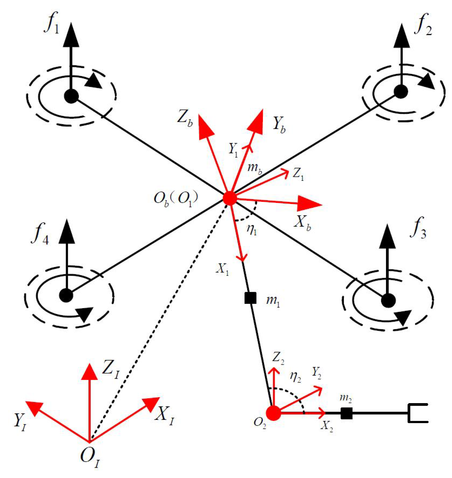
The unit quaternion q = q 0 q v T R 4 , q = 1 , is used to represent the rotation of the quadrotor in this paper. Several corresponding operations are given as follows.
The quaternion multiplication:
q σ = q 0 σ 0 q v T σ v q 0 σ v + σ 0 q v S ( σ v ) q v
The relationship between rotation matrix C A B and unit quaternion q is represented by:
C A B = ( q 0 2 q v T q v ) I 3 + 2 q v q v T + 2 q 0 S ( q v )
Take the time derivative of Equation (4), we could obtain
C A B ˙ = S ω C A B
The derivative of a quaternion and the quaternion error q e are provided, respectively, as
q ˙ = q ˙ 0 q ˙ v = 1 2 q 0 ω = 1 2 q v T S ( q v ) + q 0 I 3 ω
q e = q d * q
where q d represents the desired quaternion whose conjugate is q d * = q d 0 q dv T . Moreover, ω denotes the angular rate of the system.
ω e = ω C d b ω d
q ˙ e = 1 2 q e 0 ω e = 1 2 q ev T S ( q ev ) + q e 0 I 3 ω e

3. Models of UAV

In this section, we present a mathematical description of the quadrotor UAV manipulator system model. The abstract graph is shown in Figure 1, in which the robotic arm is fixed at the geometric center of the UAV.

3.1. Kinematic Model

Figure 1 shows several coordinates in UAV that we consider.
O I : the world-fixed inertial reference frame. O b : the body-fixed reference frame centered in the quadrotor Center of Gravity (CoG). O i : the coordinate of robotic arm i, where ( i = 1 , 2 ) denotes the link number.
Moreover, several parameters definition are given as follows.
p I = [ x , y , z ] T : the absolute position of O b with respect to O I . Ψ = [ φ , θ , ψ ] T : Euler angles used for representing the UAV attitude angle. η = [ η 1 , η 2 ] T : the joint angles of the robotic arm relative to the zero position. H = [ ( p I ) T , Ψ T , η T ] T R 8 × 1 : a vector used for including all the generalized variables. p ˙ I : the absolute linear velocity of UAV described in O I . p ˙ b : the linear velocity of UAV with respect to O b . ω I = [ ω x I , ω y I , ω z I ] T : UAV’s absolute rotational velocity described in O I . ω b = [ ω x b , ω y b , ω z b ] T : the rotational velocity of UAV relative to O b . Then we could get:
p ˙ I = R b p ˙ b ω I = R t Ψ ˙ ω b = ( R b ) T ω I = ( R b ) T R t Ψ ˙ = R r Ψ ˙
where R t R 3 × 3 represents the transformation matrix for converting Euler angle rates Ψ ˙ into ω I . R b R 3 × 3 denotes the rotation matrix representing the orientation of O b relative to O I , and R r = ( R b ) T R t R 3 × 3 is used to map the derivative of Ψ into UAV angular rate expressed in O b .
Where
R b = c θ c ψ s φ s θ c ψ c φ s ψ c φ s θ c ψ + s φ s ψ c θ s ψ s φ s θ s ψ + c φ c ψ c φ s θ s ψ s φ c ψ s θ s φ c θ c φ c θ R r = 1 0 s θ 0 c φ s φ c θ 0 s φ c φ c θ
c ( · ) and s ( · ) denote cos ( · ) and sin ( · ) , respectively.
Moreover, the position and angular rate of the frame O i , which is fixed to the robotic arm, with respect to O I are provided by
p i I = p I + R b p i b ω i I = ω I + R b ω i b
where i = ( x , y , z ) . The vectors p i b , ω i b , which are expressed in O b , represent the position of O i and the angular rate of the i-th robotic arm frame with respect to O b , respectively. Additionally, more relationships are provided,
p ˙ i b = J pi η ˙ ω i b = J ri η ˙
where J pi R 2 × 2 and J ri R 2 × 2 are Jacobian matrices representing the translational and angular velocities of each robotic arm link to the η ˙ , respectively. According to Equations (12) and (13), we could get the translational and angular velocity of O i with respect to O I as
p ˙ i I = p ˙ + S ( ω I ) R b p i b + R b J pi η ˙ ω i I = ω I + R b J ri η ˙
where S ( · ) represents the skew-symmetric matrix.

3.2. Dynamic Model

In order to obtain the dynamic model of the quadrotor UAV manipulator system, the Euler-Lagrange equation is introduced.
d d t L H k L H k = u k + d k , L = K U
where k = ( 1 , , 8 ) . L: the Lagrangian with kinetic energy K and potential energy U of the integrated system. u k : the generalized driving force. d k : external disturbance applied to the system. Additionally, K could be given in detail as
K = K b + i = 1 2 K i K b = 1 2 m b ( p ˙ I ) T p ˙ I + 1 2 ( ω I ) T R b I b R b T ω I K i = 1 2 m i ( p ˙ i I ) T p ˙ i I + 1 2 ( ω i I ) T R b R i b I i R b i R b T ω i I
where m b is the quadrotor base mass, m i is the i-th robotic arm mass ( i = ( 1 , 2 ) ), I is the inertia matrix, and R i b the rotation matrix between the frame fixed to the center of mass of the i-th link and O b . Then, the total potential is provided as
U = U b + i = 1 2 U i U b = m b g e 3 T p I U i = m i g e 3 T p i I
where e 3 denotes unit vector [ 0 , 0 , 1 ] T and g represents the gravity constant. By substituting Equations (16) and (17) into Equation (15), the dynamic model of the quadrotor UAV manipulator system could be obtained as
M ( H ) H ¨ + C ( H , H ˙ ) + G ( H ) = u + d
Moreover, the total kinetic energy can be expressed:
K = 1 2 H ˙ T M ( H ) H ˙
where
M ( H ) = M 11 M 12 M 13 M 21 M 22 M 23 M 31 M 32 M 33
Details of the inertia matrix M ( H ) and Coriolis matrix C ( H , H ˙ ) can be found in [27]. The G ( H ) could be obtained via partial derivative Equation (21):
G ( H ) = U H
Express Equation (18) in detail as
M 11 M 12 M 13 M 21 M 22 M 23 M 31 M 32 M 33 p ¨ I Ψ ¨ η ¨ + G 1 G 2 G 3 + C 11 C 12 C 13 C 21 C 22 C 23 C 31 C 32 C 33 p ˙ I Ψ ˙ η ˙ = u t u r u l + d t d r d l
where u t , u r , u l represent the generalized control inputs corresponding to p I , Ψ , η . u l is not used, as we do not consider a dynamic robotic arm in this work. Vector d = [ d t , d l , d r ] T are the lumped external disturbance. As for the quadrotor attitude loop subsystem, we would transform u r to the quadrotor inputs f v = [ ω 1 2 , ω 2 2 , ω 3 2 , ω 4 2 ] T , which is a positive correlation vector with forces produced from the quadrotor propellers. Moreover, ω i represents rotor rate of quadrotor propeller ( i = 1 , 2 , 3 , 4 ) . Then, convert the generalized control inputs to the propeller rate:
u r = R r T Ξ f v
Ξ = 2 l 2 Λ T 2 l 2 Λ T 2 l 2 Λ T 2 l 2 Λ T 2 l 2 Λ T 2 l 2 Λ T 2 l 2 Λ T 2 l 2 Λ T l Λ C l Λ C l Λ C l Λ C
where Λ T and Λ C are the thrust and drag coefficients, respectively. Additionally, l denotes the distance from each motor to the quadrotor CoG.
According to Equation (22), we could obtain in detail the dynamics of the attitude loop subsystem which is the base of next section:
M 21 p ¨ I + M 22 Ψ ¨ + M 23 η ¨ + C 21 p ˙ I + C 22 Ψ ˙ + C 23 η ˙ + G 2 = u r + d r

4. Method

Based on the UAV model, the proposed control strategy is described in detail in this section. As shown in Figure 2, quadrotor attitude control problem could be briefly divided into two components: FASTESO, used for estimating and compensating the disturbance, plays a role of the feedforward loop, and Backstepping controller, built for regulating the orientation to track the desired attitude timely, plays a role of the feedback loop. Meanwhile, TD, saturation function, and fuzzy logic methods are incorporated into the whole control method.

4.1. FASTESO

UAVs with robotic arms have more model uncertainty than traditional UAVs. Additionally, UAVs usually face some other disturbances such as external wind when flying outside. Moreover, the control performance of closed loop system will be largely determined by the observation performance. Therefore, in this part, in order to enhance the performance of feedback controller, a new SMO named FASTESO is built to estimate the lumped disturbance exerted on quadrotor UAV manipulator in finite time.
As for the traditional SMO, the sign function is generally adopted as the control function, and owing to switch time and space lag the SMO performs serious chattering problem [28,29]. In order to alleviate the chattering phenomenon, the sign function is replaced by a saturation function in this work. Moreover, the chattering phenomenon would also be invited by large switching gain because when the control signal crosses the sliding surface, larger switching gain would produce faster and bigger switching control parts and perform terrible chattering phenomenon. Additionally, the invited saturation function has a slower performance than the sign function on arithmetical speed, so there would be a time delay relatively. To further settle the problems of chattering and time delay mentioned before, fuzzy logic rules are employed in FASTESO to adjust the switching gains according to the states of the sliding surface.

4.1.1. Construction of Traditional Super-Twisting Extended State Observer (STESO)

In this part, according to our previous work [30], a traditional SMESO named STESO for quadrotor UAV manipulator is constructed. In this work, the situation, in which the robotic arm keeps constant while the UAV faces external disturbances during the flight, is mainly considered: ( η ˙ = η ¨ = 0 ). That is a general scenario that the quadrotor UAV manipulator often encounters when conducting aerial tasks. Nevertheless, usually there is unwanted vibration of the equipped robotic arm caused by the high-speed motors and propellers. To consider all mentioned disturbances, the model (25) could be reconstructed as
( M 21 + Δ M 21 ) p ¨ I + ( M 22 + Δ M 22 ) Ψ ¨ + C 21 p ˙ I + ( M 23 + Δ M 23 ) Δ η ¨ + C 22 Ψ ˙ + C 23 Δ η ˙ + G 2 = u r + d r
where Δ M 21 , Δ M 22 , Δ M 23 represent model uncertainties. Δ η ˙ and Δ η ¨ , considered as a portion of model uncertainty, denote the residuals from the temporary variation of the robotic arm parameters η ˙ , η ¨ .
In order to build the observer, reconstruct the attitude dynamic Equation (26) as
M 22 Ψ ¨ = u r + d r M 21 p ¨ I Δ M 21 p ¨ I Δ M 22 Ψ ¨ ( M 23 + Δ M 23 ) Δ η ¨ C 23 Δ η ˙ C 21 p ˙ I C 22 Ψ ˙ G 2
Introduce the lumped disturbance as
d r * = d r Δ M 21 p ¨ I Δ M 22 Ψ ¨ ( M 23 + Δ M 23 ) Δ η ¨ C 23 Δ η ˙
Combining Equations (27) and (28), we get
M 22 Ψ ¨ = u r + d r * M 21 p ¨ I C 21 p ˙ I C 22 Ψ ˙ G 2
where the variable p ¨ I is measured directly from the sensors or velocity differential is too noisy to use, so TD is introduced here to estimate the system acceleration for noise alleviation. Additionally, p ˙ I and Ψ ˙ measured from the sensors are also a little noisy, in that case, TD would be used to reduce noise, too. Moreover, the items M 21 , C 21 and G 2 could be obtained in advance according to the presented UAV model. As for dynamics model (29), considering the feedback linearization method, we could reformulate the control input as
u r = u r * + M 21 p ¨ I + C 21 p ˙ I + C 22 Ψ ˙ + G 2
Combining Equations (29) and (30), we get
M 22 Ψ ¨ = u r * + d r *
When building the STESO, it is supposed that every channel is independent from each other. Therefore, only one channel will be presented here and the other two are completely identical. As for model Equation (31), the one-dimensional model for STESO design is provided as
J i Ψ ¨ i = u ri * + d ri *
Introduce a new extended state vector ζ = [ ζ 1 ζ 2 ] T , where ζ 1 = J i Ψ ˙ i and ζ 2 = d r i * , ( i = φ , θ , ψ ) . Reconstruct the model (32) as
ζ ˙ 1 = u ri * + ζ 2 ζ ˙ 2 = χ
where χ denotes the derivative of d ri * , supposed by χ < f + . It means that the differentiation of lumped disturbance is bounded.
Then, according to the work in [30], build STESO for the observable system (33) as
z ˙ 1 = z 2 + u ri * + α 1 e 1 1 2 sign ( e 1 ) z ˙ 2 = α 2 sign ( e 1 )
where z 1 and z 2 are estimations of ζ 1 and ζ 2 , respectively. e 1 = ζ 1 ζ ^ 1 and e 2 = ζ 2 ζ ^ 2 denote estimation errors. We could obtain that the system estimation errors e 1 and e 2 would converge to zero within finite time under suitable observer gains α 1 , α 2 . Moreover, the details of the convergence analysis and parameter selection rules could be found in [30].

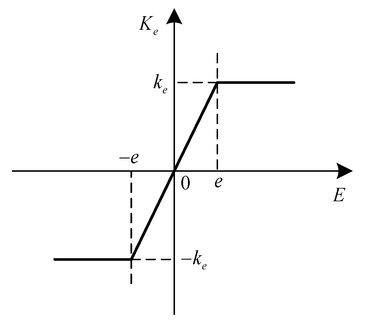
4.1.2. Saturation Function

To mitigate the chattering problem, we replace the sign function, usually expressing the discontinuous control in the observer, with a saturation function. The traditional STESO Equation (34) could be rewritten as
z ˙ 1 = z 2 + u ri * + α 1 e 1 1 2 sign ( e 1 ) z ˙ 2 = k f α 2 sat ( e 1 )
where k f is the adaptive proportional factor of switching gain generated from fuzzy logic rules which will be introduced in next part. sat ( ) represents the saturation function whose curve is shown in Figure 3, where particularly e is the difference between the real system and the estimated one. k e is the output of the saturation function. We could adjust the sliding mode effect by regulating values of e and k e . Obviously the chattering would be reduced via increasing e and decreasing k e . If e is big enough and k e is small enough, the high-frequency chattering could be avoided. However, meanwhile the robustness of the sliding mode method would also be reduced. Therefore the tuning of these parameters is a tradeoff between the chattering alleviation performance and the system robustness. Therefore, e and k e should be considered overall according to real applications.

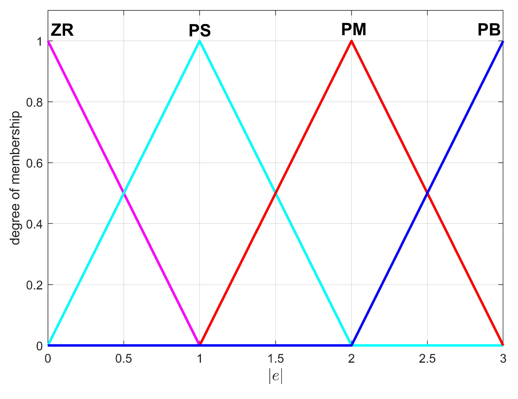
4.1.3. Adaptive Switching Gains with Fuzzy Logic Rules

The fuzzy logic controller was proposed many years ago [31]. In this part, the fuzzy rules are designed according to the fuzzy control theory for effectively optimizing the switching gain based on the states of the sliding-mode surface.
Normally, for purpose of enhancing the ability of observer on anti-disturbance and undertaking the generation of sliding mode, the sliding mode switching gain is often chosen to be too large, but this would further enhance the chattering noise in the disturbance estimation. Therefore, it is feasible to introduce the intelligent method to effectively estimate the switching gain according to the sliding mode arrival condition to alleviate the system chattering problem. For example, as the system state is far from the sliding surface, it means that the absolute value of difference e is relatively large, the proportional factor k f should be enlarged to drive the system state back. Similarly, as the system state is close to the sliding surface, proportional factor k f should be smaller.
The proposed fuzzy logic system in this work consists of one input variable and one output variable which would be quantized first. The input and output variables are divided into four fuzzy subsets. Let e = ZR PS PM PB denote the input variable and k f = ZR PS PM PB represent the output variable, respectively. Each rank is depicted by a membership function of trigonometric function, as shown in Figure 4 and Figure 5, where the fuzzy language is defined as ZR (zero), PS (positive small), PM (positive middle), and PB (positive big).
Then define the fuzzy rules as
Rule 1: If e is PB, then k f is PB.
Rule 2: If e is PM, then k f is PM.
Rule 3: If e is PS, then k f is PS.
Rule 4: If e is ZR, then k f is ZR.
Finally, as for the fuzzy outputs, according to the work in [32], the center of gravity algorithm is adopted as the defuzzification method to convert the fuzzy subset duty cycle changes to real numbers, which is given as
k f = 0 3 k f · μ out · d k f 0 3 μ out · d k f
where μ out represents the resulting output membership function. It takes every rule into account performing the union of the resulting output membership function μ out , i of each Rule i ( i = 1 , , 4 ) , which means the maximum operation between them.

4.2. Attitude Controller

In order to achieve high-precision attitude stabilization in the presence of external wind and model uncertainties, a backstepping controller is built here combined with FASTESO for UAV attitude system. The main objective of this part is to guarantee that the state of attitude q and angular rate w converge to the reference values q d and w d in real time. As this part is identical to our previous work [30] except the UAV model, which would not impact the controller design. Therefore we are not going to describe it in detail.
According to the authors of [30], the control signal vector u r is designed as
u r = M 22 ( S ( ω e ) C d b ω d C d b ω ˙ d ) + M 21 p ¨ I + M 23 η ¨ + C 21 p ˙ I + C 22 Ψ ˙ + C 23 η ˙ + G 2 M 22 K b 1 q ˙ ev q ev K b 2 ω ˜ e d r ^
where d ^ r is the estimated result of disturbance from FASTESO. Additionally, like what we did at FASTESO, TD will also be adopted here to process several variables in Equation (37) to reduce noise. Moreover, K b 1 , K b 2 are controller gains to be designed, and ω e , ω ˜ e , and q ev are defined in Equation (38), details of which can be found in [30].
ω e = ω C d b ω d ω ˜ e = ω e + K b 1 q ev q e = q 0 q ev T q e = q d * q

5. Simulation

In this section, the performance of proposed FASTESO-based control method is validated on the PX4/Gazebo platform [33], which provides simulations of physics close to the real world. A manually designed scalable disturbance, which includes a sudden change in some special points, is defined in Equation (39) and adopted in the simulations. Moreover, its amplitude could be adjusted by a. The main nominal coefficients of the quadrotor base are generated by the online toolbox of Quan and Dai [34] given in Table 1.
d e = a ( 0.25 ( 0.02 sin ( 0.1 π t ) ) + 0.015 sin ( 0.3 π t 5 ) 0.02 )

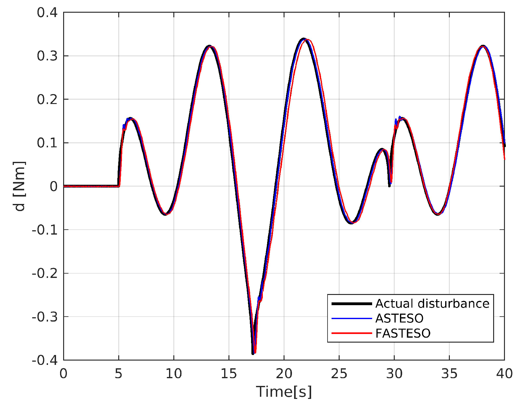
5.1. CASE 1 (Observers Performance Comparison)

In this section, several comparison simulations on observer performance of disturbance estimation are conducted.

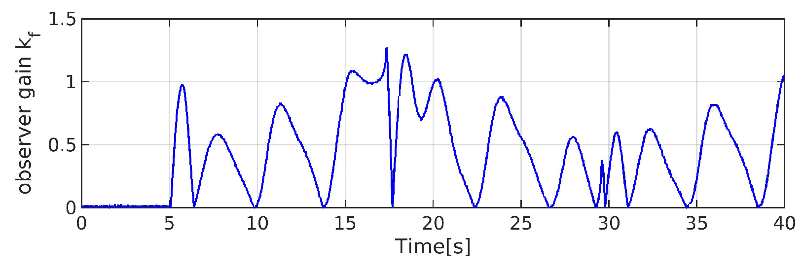
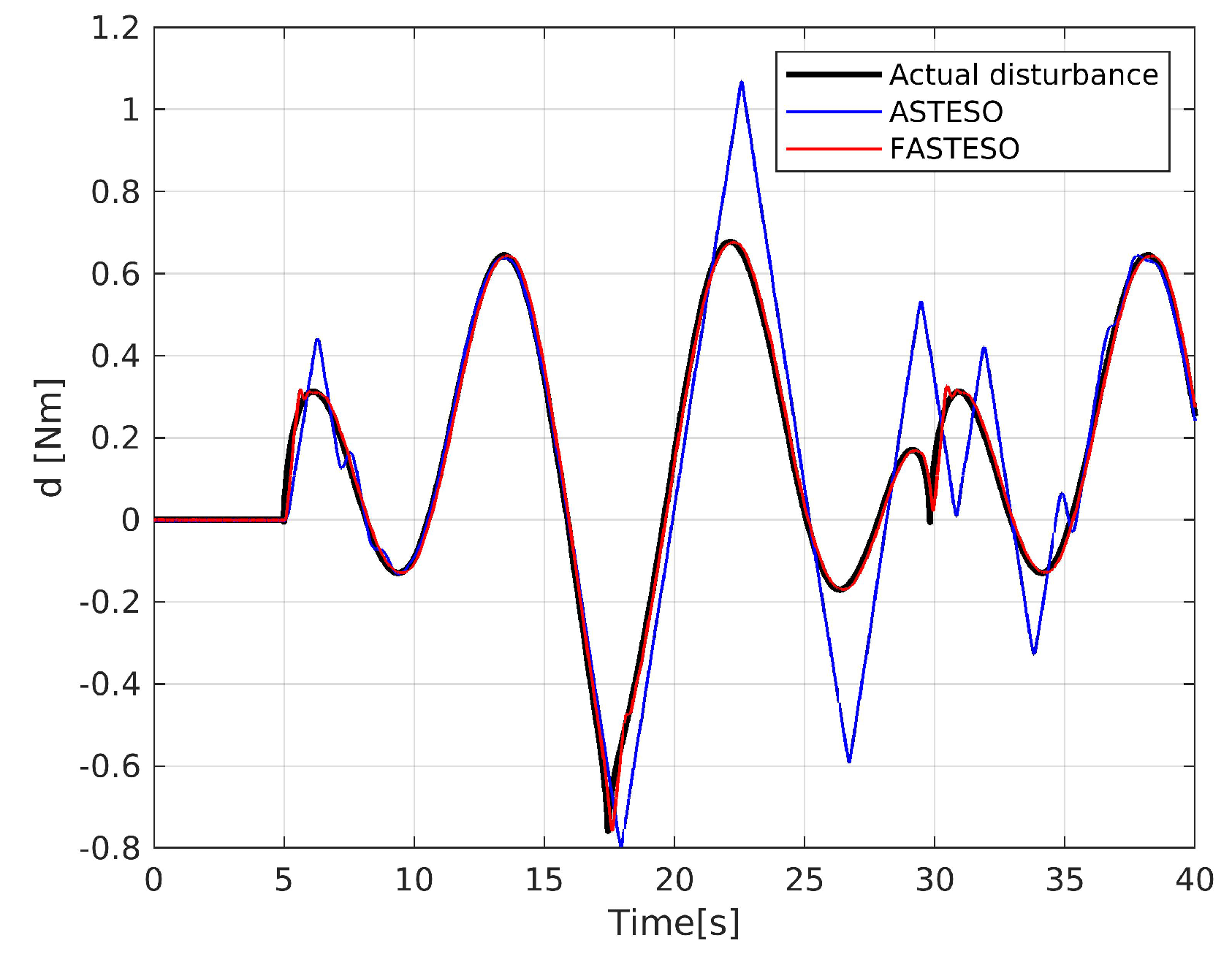
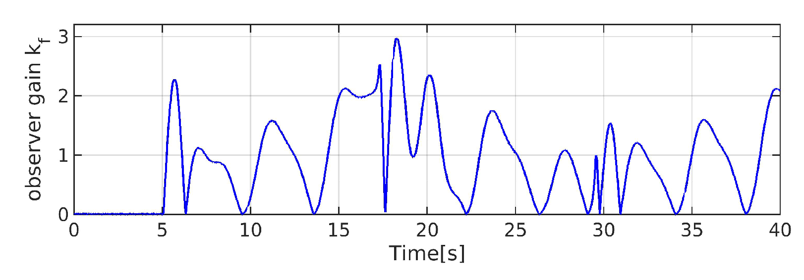
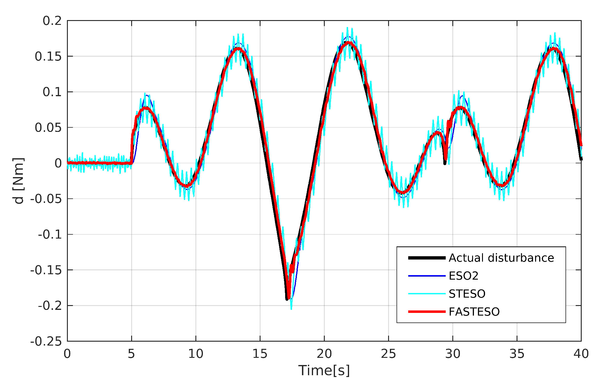
5.1.1. Domestic Observers Comparison

To verify the effectiveness of the proposed fuzzy logic rules for adaptively adjusting the observer gain to cope with disturbances with different amplitudes, comparative simulations are conducted for a quadrotor UAV manipulator performing a hovering flight with the manually designed scalable disturbance (39) between FASTESO and ASTESO combined with a backstepping controller (BAC). The ASTESO is defined as a simplified version of FASTESO, which is not equipped with adaptive gain under fuzzy logic rules. Their coefficients are given as FASTESO: α 1 = diag (0.4,0.4,0.5); α 2 = diag ( 0.7 , 0.7 , 0.9 ) ; e = 0.0001 ; k e = 0.05 . ASTESO: α 1 = diag (0.4,0.4,0.5); α 2 = diag ( 0.7 , 0.7 , 0.9 ) . BAC: K b 1 = diag ( 5 , 5 , 8 ) ; K b 2 = diag ( 3 , 3 , 4 ) . The simulations are divided into two groups classified by different scalars of disturbances, a = 10 , 20 . The corresponding results could be found in Figure 6, Figure 7, Figure 8 and Figure 9.
As shown in Figure 6, both FASTESO and ASTESO have good estimation performance under scalar a = 10 . The resultant observer gain of FASTESO is described in Figure 7. Nevertheless, the ASTESO starts to break down when the disturbance is larger, which could be found in Figure 8. Under a = 20 , the ASTESO fails to follow the larger disturbance, but the proposed FASTESO still performs well. This is because the fixed parameter of ASTESO is not big enough to estimate the disturbance with the amplitude in Figure 8. As shown in Figure 9, the adaptive gain of FASTESO also shows why it is effective under disturbances with different amplitudes. To summarize, this part shows that the proposed FASTESO could estimate a wider range of disturbance thanks to the fuzzy logic rules for adaptive observer gain.

5.1.2. Various Observers Comparison

To demonstrate the effectiveness of the introduction of the saturation function into SMO, a simulation similar with last part is conducted under FASTESO with an applied disturbance under a = 5 shown in Figure 10. Meanwhile the 2nd-order linear ESO (ESO2) and STESO are also invited for comparison. The parameters of the mentioned observers are listed. FASTESO: α 1 = diag (0.4,0.4,0.5); α 2 = diag ( 0.7 , 0.7 , 0.9 ) ; e = 0.0001 ; k e = 0.05 . ESO2: k 1 = diag (4.5,4.5,6.5); k 2 = diag (22,22,28); k 3 = diag (5,5,8); STESO: α 1 = diag (0.2,0.2,0.3); α 2 = diag ( 0.3 , 0.3 , 0.4 ) ; BAC: K b 1 = diag ( 5 , 5 , 8 ) ; K b 2 = diag ( 3 , 3 , 4 ) .
From the response results in Figure 10, we could find that FASTESO has a perfect performance on estimation even at the special point with a sudden change. Although the curve under ESO2 could usually follow the actual value, it performs an overestimation near the peak. As for STESO, it could follow the fast variation of disturbance; however, it has a terrible chattering problem which is also the main reason for the introduction of saturation function in this work. To summarize, the FASTESO performs well at all range of disturbance ( a = 5 , 10 , 20 ). Meanwhile, it follows better than other traditional observers under varied disturbance.

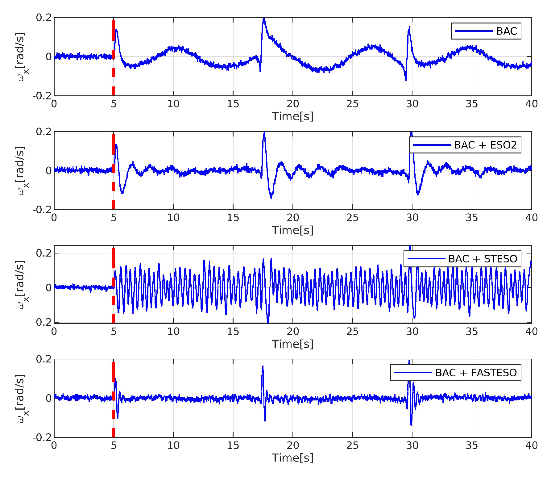
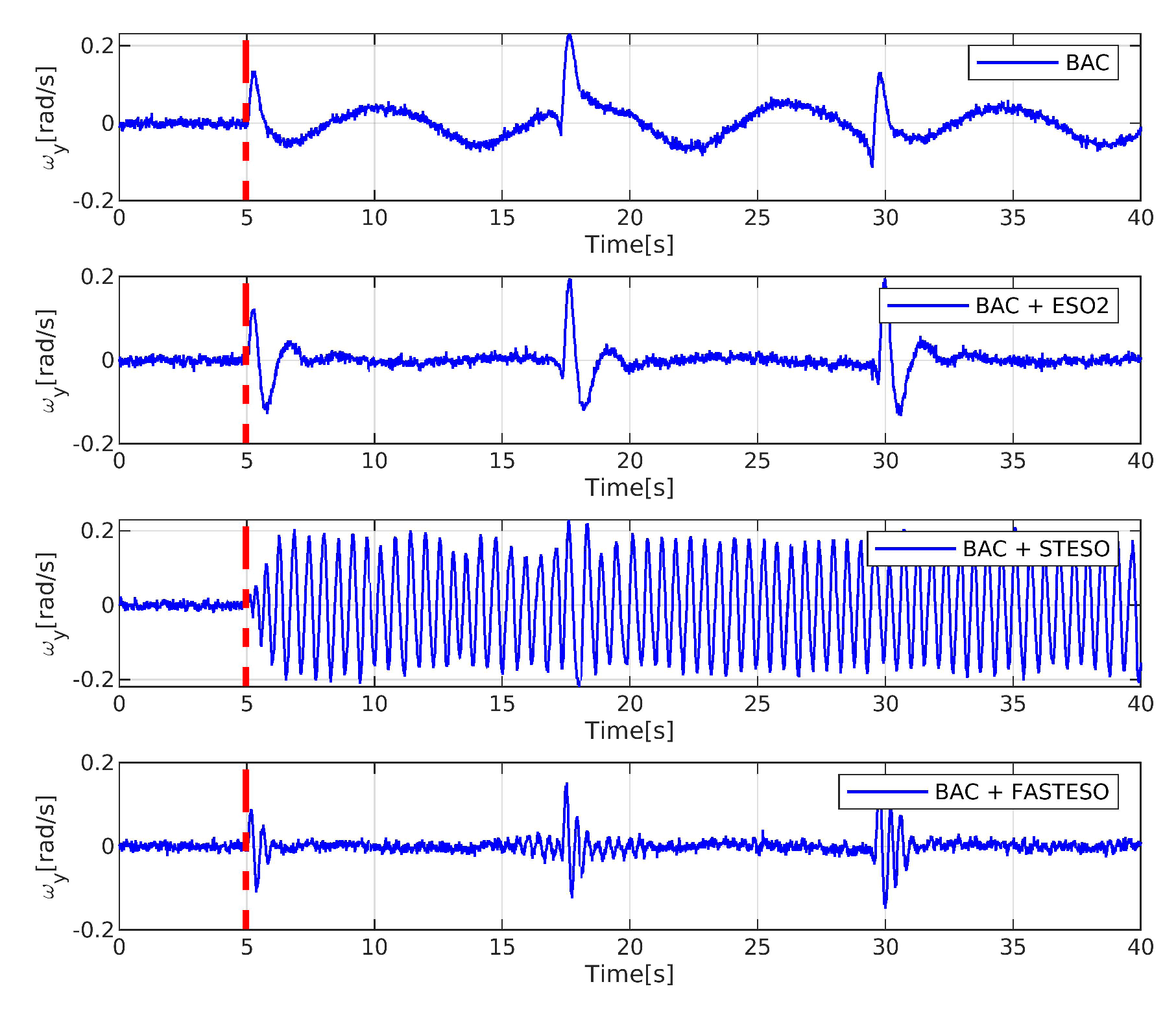
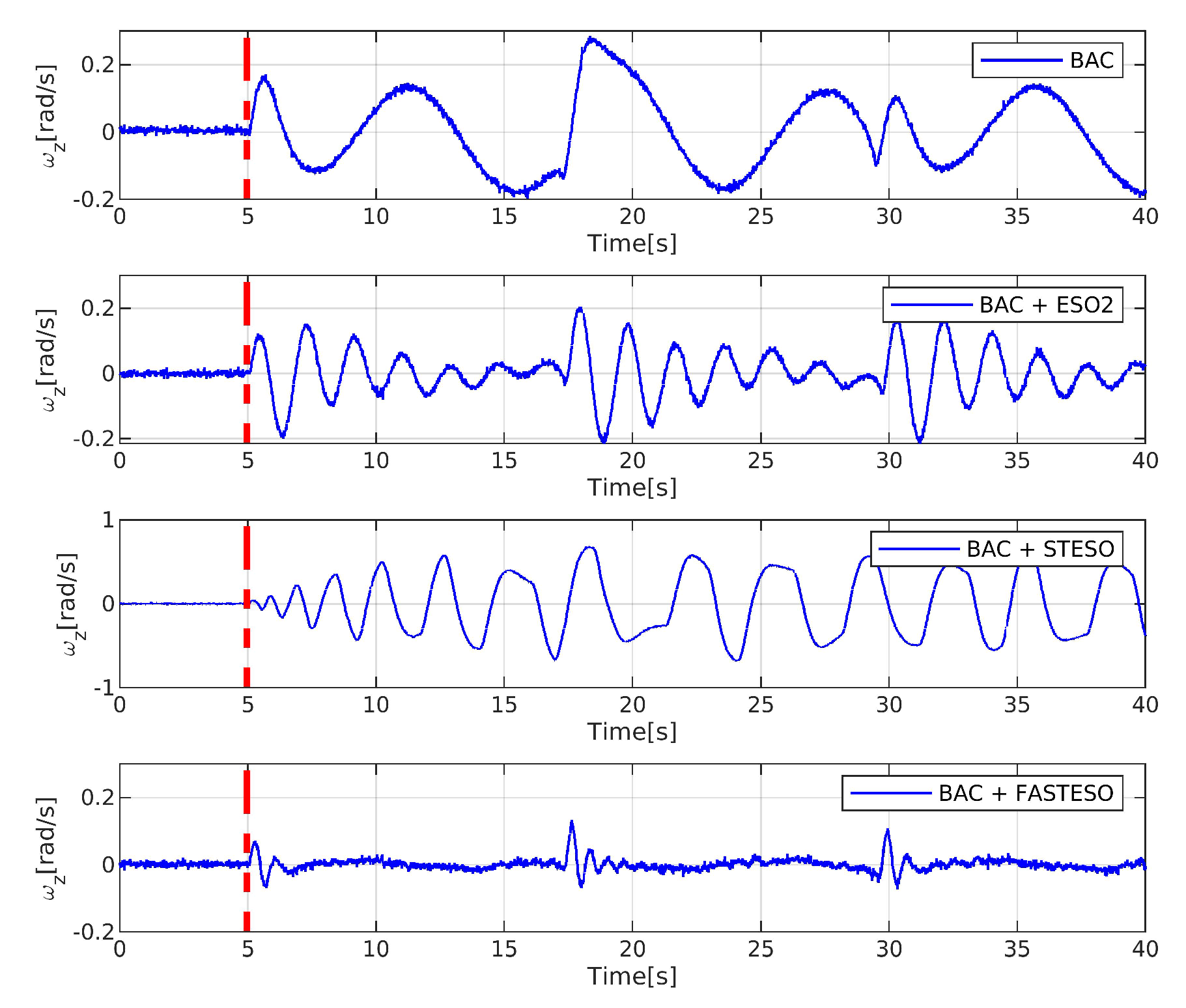
5.2. CASE 2 (Composite Comparison)
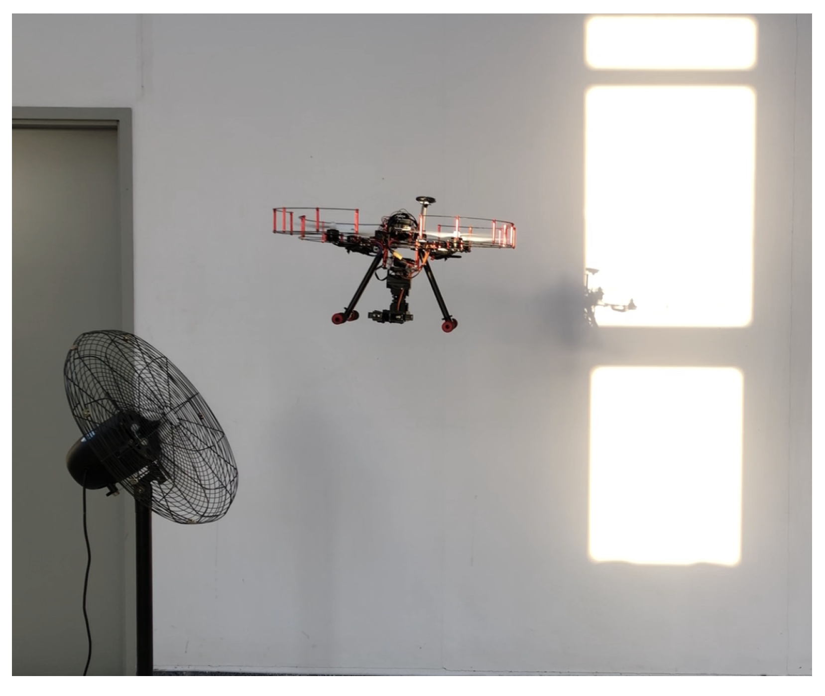
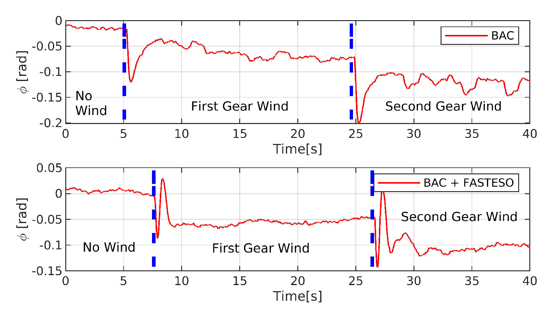
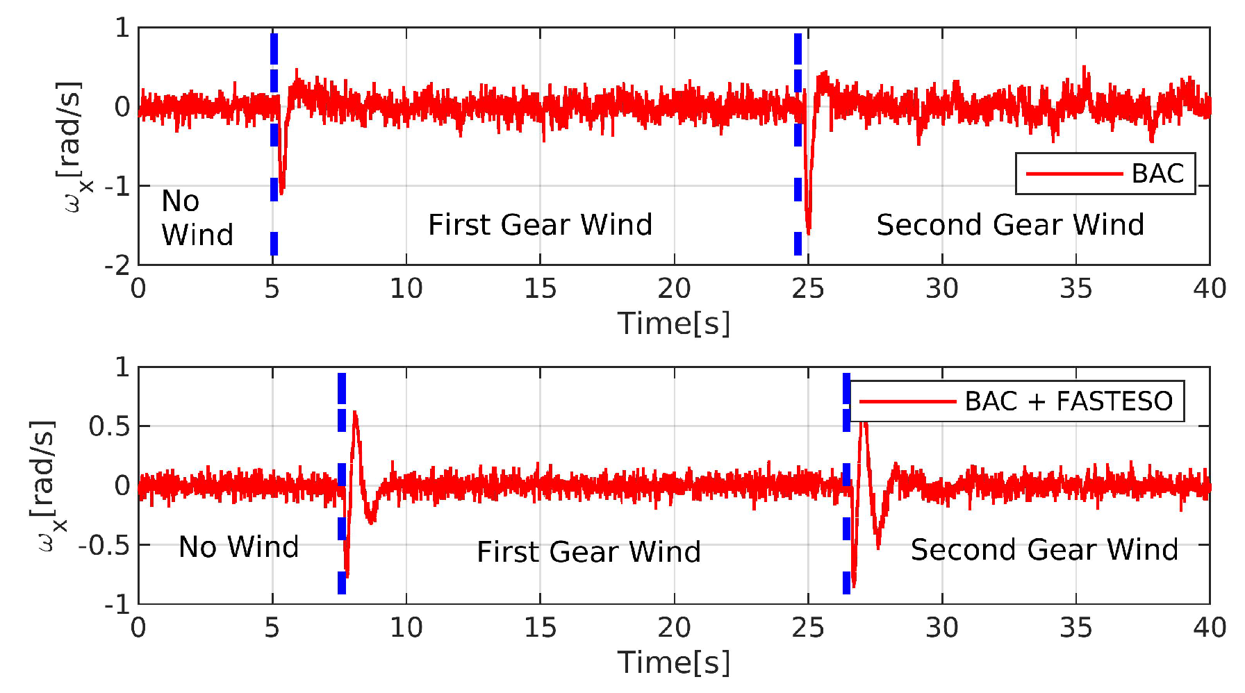
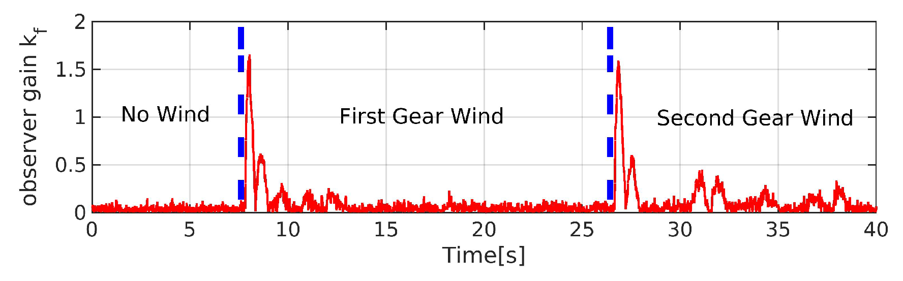
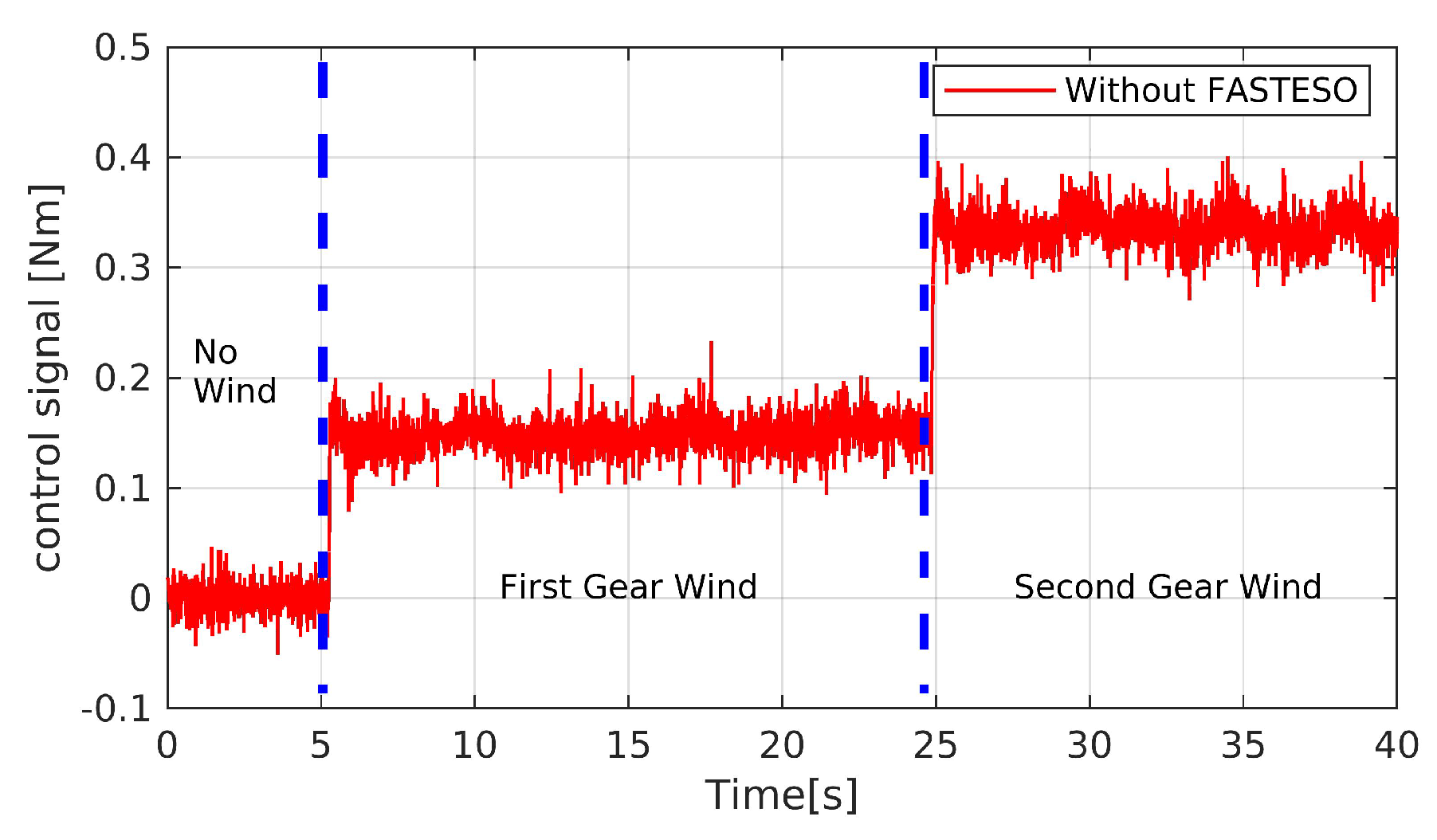
To further illustrate the effectiveness of the whole proposed control strategy, we would show all-sided simulation results from Section 5.1.2. Moreover, a single backstepping controller without any observer is also conducted on quadrotor UAV manipulator system for comparison. Three-axis components of disturbance torque d r = d r φ d r θ d r ψ T are equal and shown in Figure 10, which are applied on the UAV simultaneously. The result curves of both attitude and angular rate are shown in Figure 11, Figure 12, Figure 13, Figure 14, Figure 15 and Figure 16.
We could easily find that, without an observer, the single BAC has biggest attitude offset and angular rate fluctuation, which proves its bad robustness under disturbances. Specifically, the attitude curves even follows the applied torque disturbance well and angular rate has a dramatic change at special points. As for BAC+ESO2, although the estimation value follows the disturbance well to some extent, it has a performance of drastic change on both attitude and angular rate at peak point owing to the over estimation near the peak. As for BAC+STESO, in spite of the good performance of STESO on following the disturbance, it has a terrible chattering phenomenon and leads to a mess on UAV system. Compared to other situations, the UAV under BAC+FASTESO has the best performance on both attitude offset and angular rate fluctuation with varied torque disturbance.

6. Experiment

In this section, to verify the effectiveness of the whole proposed method, the quadrotor UAV manipulator is assigned to conduct a hovering task beside an electrical fan, which could generate several level gear wind as torque disturbance acting on the UAV system. BAC+FASTESO is adopted for UAV disturbance rejection test, meanwhile a single BAC without any observer is also conducted for comparison. The experimental scene is shown in Figure 17. The whole proposed control scheme is built in Pixhawk [35]. The parameters are chosen as follows. For BAC+FASTESO: α 1 = diag ( 0.2 , 0.2 , 0.3 ) ; α 2 = diag (0.3,0.3,0.4) e = 0.001 ; k e = 0.1 ; K b 1 = diag ( 3 , 3 , 5 ) ; K b 2 = diag (2,2,2.5). For BAC: K b 1 = diag ( 6 , 6 , 9 ) ; K b 2 = diag (3.5,3.5,5).
The fan is placed to mainly apply the external torque in roll channel. The results of UAV hovering under first and second gear wind are shown in Figure 18, Figure 19, Figure 20, Figure 21, Figure 22 and Figure 23. We found that the attitude of hovering UAV changes following the variation of wind gear. Moreover, the attitude vibration offset is reduced by help of FASTESO compared to the situation with single BAC. Meanwhile, the angular rate fluctuation is also reduced. They intuitively verify the effectiveness of FASTESO. Additionally, Figure 22 and Figure 23 show the control output generated only from BAC in the control situations single BAC and BAC+FASTESO, respectively. We could find that the control signal is around zero with FASTESO; however, the control signal is impacted so much owing to external disturbance in situation without any observer. Moreover, the controller gain in BAC+FASTESO could keep smaller to make the whole system stable thanks to the disturbance estimation and compensation from FASTESO, which also contributes to the better performance of BAC+FASTESO. Meanwhile, the estimation of the lumped disturbance including external wind and model uncertainties is shown in Figure 20. Although we do not know the ground truth of the torque disturbance generated from the fan and model uncertainties to verify if the estimation result in Figure 20 is right or not, according to Figure 20 and Figure 22, we could see that their results are almost the same, which also demonstrates the effectiveness of FASTESO to an extent.

7. Conclusions

In this study, a new observer named FASTESO is proposed, which is incorporated with the saturation function, TD and fuzzy logic rules. Combined with backstepping controller, the whole control scheme for the quadrotor UAV manipulator system is finally built for rejection of lumped disturbance including external wind and model uncertainties. The effectiveness of the whole control structure is veritied in both several simulations and experiments.
In the future, we would pay more attention to the estimation separation of the model uncertainties from the external disturbance.

Author Contributions

Conceptualization, R.J.; writing—original draft preparation, R.J.; software, R.J. and Y.R.; validation, R.J. and Y.R.; methodology, R.J. and M.D.; writing—review and editing, R.J., W.C. and M.D.; supervision, W.C. All authors have read and agreed to the published version of the manuscript.

Funding

This work was supported by National Key R&D Program of China under grant number 2017YFB1302503 and 2019YFB1310802.

Conflicts of Interest

The authors declare no conflicts of interest.

Abbreviations

Additional abbreviation illustration:
FASTESOFuzzy adaptive saturation super-twisting extended state observer

References

  1. Premachandra, C.; Ueda, D.; Kato, K. Speed-Up Automatic Quadcopter Position Detection by Sensing Propeller Rotation. IEEE Sens. J. 2018, 19, 2758–2766. [Google Scholar] [CrossRef]
  2. Nakajima, K.; Premachandra, C.; Kato, K. 3D environment mapping and self-position estimation by a small flying robot mounted with a movable ultrasonic range sensor. J. Electr. Syst. Inf. Technol. 2017, 4, 289–298. [Google Scholar] [CrossRef]
  3. Premachandra, C.; Otsuka, M.; Gohara, R.; Ninomiya, T.; Kato, K. A study on development of a hybrid aerial/terrestrial robot system for avoiding ground obstacles by flight. IEEE/CAA J. Autom. Sin. 2018, 6, 327–336. [Google Scholar] [CrossRef]
  4. Ryll, M.; Muscio, G.; Pierri, F.; Cataldi, E.; Antonelli, G.; Caccavale, F.; Bicego, D.; Franchi, A. 6D interaction control with aerial robots: The flying end-effector paradigm. Int. J. Robot. Res. 2019, 38, 1045–1062. [Google Scholar] [CrossRef] [Green Version]
  5. Kim, S.; Seo, H.; Shin, J.; Kim, H.J. Cooperative aerial manipulation using multirotors with multi-dof robotic arms. IEEE/ASME Trans. Mechatronics 2018, 23, 702–713. [Google Scholar] [CrossRef]
  6. Jiao, R.; Dong, M.; Chou, W.; Yu, H.; Yu, H. Autonomous Aerial Manipulation Using a Hexacopter Equipped with a Robotic Arm. In Proceedings of the 2018 IEEE International Conference on Robotics and Biomimetics (ROBIO), Kuala Lumpur, Malaysia, 12–15 December 2018; pp. 1502–1507. [Google Scholar]
  7. Ruggiero, F.; Trujillo, M.A.; Cano, R.; Ascorbe, H.; Viguria, A.; Peréz, C.; Lippiello, V.; Ollero, A.; Siciliano, B. A multilayer control for multirotor UAVs equipped with a servo robot arm. In Proceedings of the 2015 IEEE international conference on robotics and automation (ICRA), Seattle, WA, USA, 26–30 May 2015; pp. 4014–4020. [Google Scholar]
  8. Jiao, R.; Chou, W.; Ding, R.; Dong, M. Adaptive robust control of quadrotor with a 2-degree-of-freedom robotic arm. Adv. Mech. Eng. 2018, 10, 1687814018778639. [Google Scholar] [CrossRef]
  9. Alexis, K.; Papachristos, C.; Siegwart, R.; Tzes, A. Robust model predictive flight control of unmanned rotorcrafts. J. Intell. Robot. Syst. 2016, 81, 443–469. [Google Scholar] [CrossRef]
  10. Achtelik, M.; Bierling, T.; Wang, J.; Höcht, L.; Holzapfel, F. Adaptive control of a quadcopter in the presence of large/complete parameter uncertainties. In Proceedings of the Infotech@ Aerospace 2011, St. Louis, MO, USA, 29–31 March 2011; p. 1485. [Google Scholar]
  11. Chen, W.H.; Yang, J.; Guo, L.; Li, S. Disturbance-observer-based control and related methods—An overview. IEEE Trans. Ind. Electron. 2015, 63, 1083–1095. [Google Scholar] [CrossRef] [Green Version]
  12. Cristofaro, A.; Johansen, T.A. Fault tolerant control allocation using unknown input observers. Automatica 2014, 50, 1891–1897. [Google Scholar] [CrossRef]
  13. Pu, Z.; Yuan, R.; Yi, J.; Tan, X. A class of adaptive extended state observers for nonlinear disturbed systems. IEEE Trans. Ind. Electron. 2015, 62, 5858–5869. [Google Scholar] [CrossRef]
  14. Kim, S.; Choi, S.; Kim, H.; Shin, J.; Shim, H.; Kim, H.J. Robust control of an equipment-added multirotor using disturbance observer. IEEE Trans. Control Syst. Technol. 2017, 26, 1524–1531. [Google Scholar] [CrossRef]
  15. Wang, C.; Song, B.; Huang, P.; Tang, C. Trajectory tracking control for quadrotor robot subject to payload variation and wind gust disturbance. J. Intell. Robot. Syst. 2016, 83, 315–333. [Google Scholar] [CrossRef]
  16. Chen, M.; Xiong, S.; Wu, Q. Tracking flight control of quadrotor based on disturbance observer. IEEE Trans. Syst. Man, Cybern. Syst. 2019. [Google Scholar] [CrossRef]
  17. Mokhtari, M.R.; Cherki, B.; Braham, A.C. Disturbance observer based hierarchical control of coaxial-rotor UAV. ISA Trans. 2017, 67, 466–475. [Google Scholar] [CrossRef]
  18. Wang, L.; Su, J. Robust disturbance rejection control for attitude tracking of an aircraft. IEEE Trans. Control Syst. Technol. 2015, 23, 2361–2368. [Google Scholar] [CrossRef]
  19. Han, J. From PID to active disturbance rejection control. IEEE Trans. Ind. Electron. 2009, 56, 900–906. [Google Scholar] [CrossRef]
  20. Liu, J.; Vazquez, S.; Wu, L.; Marquez, A.; Gao, H.; Franquelo, L.G. Extended state observer-based sliding-mode control for three-phase power converters. IEEE Trans. Ind. Electron. 2016, 64, 22–31. [Google Scholar] [CrossRef] [Green Version]
  21. Madoński, R.; Herman, P. Survey on methods of increasing the efficiency of extended state disturbance observers. ISA Trans. 2015, 56, 18–27. [Google Scholar] [CrossRef]
  22. Muñoz, F.; Bonilla, M.; Espinoza, E.S.; González, I.; Salazar, S.; Lozano, R. Robust trajectory tracking for unmanned aircraft systems using high order sliding mode controllers-observers. In Proceedings of the 2017 International Conference on Unmanned Aircraft Systems (ICUAS), Miami, FL, USA, 13–16 June 2017; pp. 346–352. [Google Scholar]
  23. Cai, W.; She, J.; Wu, M.; Ohyama, Y. Disturbance suppression for quadrotor UAV using sliding-mode-observer-based equivalent-input-disturbance approach. ISA Trans. 2019, 92, 286–297. [Google Scholar] [CrossRef]
  24. Shi, D.; Wu, Z.; Chou, W. Super-twisting extended state observer and sliding mode controller for quadrotor UAV attitude system in presence of wind gust and actuator faults. Electronics 2018, 7, 128. [Google Scholar] [CrossRef] [Green Version]
  25. Kim, H.; Son, J.; Lee, J. A high-speed sliding-mode observer for the sensorless speed control of a PMSM. IEEE Trans. Ind. Electron. 2010, 58, 4069–4077. [Google Scholar]
  26. Rong, Y.; Jiao, R.; Kang, S.; Chou, W. Sigmoid Super-Twisting Extended State Observer and Sliding Mode Controller for Quadrotor UAV Attitude System With Unknown Disturbance. In Proceedings of the 2019 IEEE International Conference on Robotics and Biomimetics (ROBIO), Dali, China, 6–8 December 2019; pp. 2647–2653. [Google Scholar]
  27. Lippiello, V.; Ruggiero, F. Cartesian impedance control of a UAV with a robotic arm. IFAC Proc. Vol. 2012, 45, 704–709. [Google Scholar] [CrossRef] [Green Version]
  28. Zhang, Z.; Xu, H.; Xu, L.; Heilman, L.E. Sensorless direct field-oriented control of three-phase induction motors based on “Sliding Mode" for washing-machine drive applications. IEEE Trans. Ind. Appl. 2006, 42, 694–701. [Google Scholar] [CrossRef]
  29. Kang, K.L.; Kim, J.M.; Hwang, K.B.; Kim, K.H. Sensorless control of PMSM in high speed range with iterative sliding mode observer. In Proceedings of the Nineteenth Annual IEEE Applied Power Electronics Conference and Exposition, 2004 (APEC’04), Anaheim, CA, USA, 22–26 February 2004; Volume 2, pp. 1111–1116. [Google Scholar]
  30. Jiao, R.; Wang, Z.; Chu, R.; Dong, M.; Rong, Y.; Chou, W. An Intuitional End-to-End Human-UAV Interaction System for Field Exploration. Front. Neurorobot. 2019, 13, 117. [Google Scholar] [CrossRef] [PubMed]
  31. Lee, C.C. Fuzzy logic in control systems: Fuzzy logic controller. I. IEEE Trans. Syst. Man, Cybern. 1990, 20, 404–418. [Google Scholar] [CrossRef] [Green Version]
  32. Palm, R. Robust control by fuzzy sliding mode. Automatica 1994, 30, 1429–1437. [Google Scholar] [CrossRef]
  33. Meier, L.; Honegger, D.; Pollefeys, M. PX4: A node-based multithreaded open source robotics framework for deeply embedded platforms. In Proceedings of the 2015 IEEE international conference on robotics and automation (ICRA), Seattle, WA, USA, 26–30 May 2015; pp. 6235–6240. [Google Scholar]
  34. Quan, Q. Flight Performance Evaluation of UAVs. 2018. Available online: http://flyeval.com/ (accessed on 15 April 2020).
  35. Meier, L.; Tanskanen, P.; Heng, L.; Lee, G.H.; Fraundorfer, F.; Pollefeys, M. PIXHAWK: A micro aerial vehicle design for autonomous flight using onboard computer vision. Auton. Robot. 2012, 33, 21–39. [Google Scholar] [CrossRef]
Figure 1. Quadrotor and robotic arm system with coordinate reference frames.
Applsci 10 03719 g001
Figure 2. Whole control structure of the proposed method.
Applsci 10 03719 g002
Figure 3. Sketch of the saturation function.
Applsci 10 03719 g003
Figure 4. Fuzzy input membership functions.
Applsci 10 03719 g004
Figure 5. Fuzzy output membership functions.
Applsci 10 03719 g005
Figure 6. Estimation results from ASTESO and fuzzy adaptive saturation super-twisting extended state observer (FASTESO) with scalar a = 10 .
Applsci 10 03719 g006
Figure 7. Observer gain of FASTESO during adaptation process with scalar a = 10 .
Applsci 10 03719 g007
Figure 8. Estimation results from ASTESO and FASTESO with scalar a = 20 .
Applsci 10 03719 g008
Figure 9. Observer gain of FASTESO during adaptation process with scalar a = 20 .
Applsci 10 03719 g009
Figure 10. Estimation results from ESO2, STESO, and FASTESO with scalar a = 5 .
Applsci 10 03719 g010
Figure 11. Results of roll angle with unknown external torque disturbance under backstepping controller combined with nothing, ESO2, STESO and FASTESO.
Applsci 10 03719 g011
Figure 12. Results of angular rate ω x with unknown external torque disturbance under backstepping controller combined with nothing, ESO2, STESO and FASTESO.
Applsci 10 03719 g012
Figure 13. Results of pitch angle with unknown external torque disturbance under backstepping controller combined with nothing, ESO2, STESO and FASTESO.
Applsci 10 03719 g013
Figure 14. Results of angular rate ω y with unknown external torque disturbance under backstepping controller combined with nothing, ESO2, STESO and FASTESO.
Applsci 10 03719 g014
Figure 15. Results of yaw angle with unknown external torque disturbance under backstepping controller combined with nothing, ESO2, STESO and FASTESO.
Applsci 10 03719 g015
Figure 16. Results of angular rate ω z with unknown external torque disturbance under backstepping controller combined with nothing, ESO2, STESO and FASTESO.
Applsci 10 03719 g016
Figure 17. Experimental scene.
Applsci 10 03719 g017
Figure 18. Experimental results of attitude with BAC and BAC+FASTESO under external wind.
Applsci 10 03719 g018
Figure 19. Experimental results of angular rate with BAC and BAC+FASTESO under external wind.
Applsci 10 03719 g019
Figure 20. Disturbance estimation result from FASTESO.
Applsci 10 03719 g020
Figure 21. Observer gain of FASTESO during adaptation process.
Applsci 10 03719 g021
Figure 22. Control output signal only from BAC without FASTESO.
Applsci 10 03719 g022
Figure 23. Control output signal only from BAC with FASTESO.
Applsci 10 03719 g023
Table 1. Quadrotor base coefficients used in simulation.
CoefficientsDescriptionValue
m b Mass of the quadrotor base1.8 kg
J b x Pitch inertia 1.319 × 10 2 kg · m 2
J b y Roll inertia 1.319 × 10 2 kg · m 2
J b z Yaw inertia 2.283 × 10 2 kg · m 2
lQuadrotor base size0.205 m

