Article

An Artificial Intelligence Approach to Prediction of Corn Yields under Extreme Weather Conditions Using Satellite and Meteorological Data

1
Geomatics Research Institute, Pukyong National University, Busan 48513, Korea
2
Climate Change and Agro-Ecology Division, National Institute of Agricultural Sciences, Jeollabuk-do 55365, Korea
3
Nano Weather Incorporation, Gyeonggi-do 13449, Korea
4
IBS Center for Climate Physics and Department of Atmospheric Sciences, Pusan National University, Busan 46241, Korea
5
Department of Applied Plant Science, Chonnam National University, Gwangju 61186, Korea
6
Department of Spatial Information Engineering, Pukyong National University, Busan 48513, Korea
*
Author to whom correspondence should be addressed.
Appl. Sci. 2020, 10(11), 3785; https://doi.org/10.3390/app10113785
Submission received: 29 March 2020 / Revised: 19 May 2020 / Accepted: 26 May 2020 / Published: 29 May 2020
(This article belongs to the Special Issue Machine Learning Techniques Applied to Geospatial Big Data)

Abstract

:
This paper describes the development of an optimized corn yield prediction model under extreme weather conditions for the Midwestern United States (US). We tested six different artificial intelligence (AI) models using satellite images and meteorological data for the dominant growth period. To examine the effects of extreme weather events, we defined the drought and heatwave by considering the characteristics of corn growth and selected the cases for sensitivity tests from a historical database. In particular, we conducted an optimization for the hyperparameters of the deep neural network (DNN) model to ensure the best configuration for accuracy improvement. The result for drought cases showed that our DNN model was approximately 51–98% more accurate than the other five AI models in terms of root mean square error (RMSE). For the heatwave cases, our DNN model showed approximately 30–77% better accuracy in terms of RMSE. The correlation coefficient was 0.954 for drought cases and 0.887–0.914 for heatwave cases. Moreover, the accuracy of our DNN model was very stable, despite the increases in the duration of the heatwave. It indicates that the optimized DNN model can provide robust predictions for corn yield under conditions of extreme weather and can be extended to other prediction models for various crops in future work.

1. Introduction

Since the 18th century, greenhouse gas emissions have been increasing as a result of industrialization and other human activity, leading to global warming and climate change. According to the Intergovernmental Panel on Climate Change (IPCC) Fifth Assessment Report (AR5), global average temperatures would rise by approximately 3.7 °C around the end of the 21st century because of global warming. Also, the frequency of high temperatures will increase further [1].
Global climate change causes a variety of extreme weather conditions, such as drought, heat and cold waves, and heavy rain, which have broad impacts on ecosystems and human society. Extreme weather phenomena have become increasingly frequent; however, it is difficult to predict due to the variability of the patterns of climate change on a global scale. Moreover, climate change is very closely related to water supply and food security. In 2010, more than 20% of Russian agricultural areas were affected by drought and heatwave; in response, the Russian government issued a wheat embargo in 2010–2011, leading to increases of up to 50% in the international wheat price [2,3]. Thus, extreme weather can trigger spikes in crop prices, leading to instability in the global food supply [4]. In the season when grain filling occurs, drought and heatwaves can have acute effects on crop growth and production [5,6]. Therefore, developing a reliable crop yield model is essential for deciding agricultural policy and ensuring food security.
Lobell et al. [7] mentioned that global corn and soybean yields could drop by approximately 5.5% and 3.8%, respectively, because of climate change. Teixeira et al. [5] presented that substantial crop yield losses due to extreme temperatures can seriously affect the global food supply. Lesk et al. [4] showed that drought and heatwave reduced national cereal production by 9–10%; the effects of drought lasted longer than those of heatwave, reducing both crop yield and harvested area. Qian et al. [8] analyzed climate change impacts on the yields of spring wheat, canola, and maize in Canada using multiple crop models under four different scenarios for global warming levels: 1.5 °C, 2.0 °C, 2.5 °C, and 3.0 °C. The results show that the yield changes would be various according to crop type. Small increases for canola and spring wheat and some decrease for maize would be expected under the warming scenarios. These previous studies demonstrated the impacts of extreme weather on actual crop yields, but they did not sufficiently present the prediction capability of the model under extreme weather conditions. Although challenging, crop yield prediction can provide useful information for adapting to changing Earth environments. A robust model for predicting crop yields under extreme weather conditions is needed for future agricultural management.
As efficient ways to predict crop yield, artificial intelligence (AI) models such as random forest (RF), support vector machine (SVM), and deep neural network (DNN) have been examined in many studies. Jeong et al. [9] used climate and soil data for the prediction of wheat and corn yields and showed that the accuracy of the AI model was better than that of classic linear equations. Kuwata and Shibasaki [10,11] used vegetation indices and climate data for corn yield prediction in the United States (US); they mentioned that the result from a DNN model was best among multiple AI models. Kim et al. [12] examined six AI models for predicting crop yield in the Midwestern US, which showed that an optimized DNN model outperformed the other five models. However, the performance of AI models for crop yield prediction may depend on the data used in the experiments. Particularly under extreme weather conditions, the dataset can have somewhat different characteristics from the usual pattern. So, the crop yield predictability of various AI models under unexpected weather conditions should be examined objectively, but previous AI studies did not focus on a comparative evaluation of AI models concerning rapid climate change.
In this study, we conducted comprehensive performance tests for multiple AI models to predict corn yield under extreme weather conditions in the Midwestern US. Six different AI models included multivariate adaptive regression spline (MARS), SVM, RF, extremely randomized tree (ERT), artificial neural network (ANN), and DNN. We configured each model through the optimization of hyperparameters and compared the validation statistics for drought and heatwave cases. For this, we prepared the input data, including satellite-based vegetation indices and meteorological data for July and August (the dominant growth period). Then, we constructed a match-up database using high-resolution maps for crop types and selected cases of extreme weather conditions such as drought and heatwave. Two types of blind tests, such as leave-one-year-out and 10-fold cross-validation, were conducted to evaluate the accuracy of these models under conditions of drought and heatwave. This study concentrated on corn yields in the Midwestern US in 2006–2015.

2. Study Area and Data

2.1. Study Area

Corn, which is among the world’s top three grain crops, has substantial importance for the global economy due to its various uses. The US is the largest grain producer and exporter, supplying approximately 40% of global annual corn production [13,14]. Hence, we focused on the five US states (Illinois with 102 counties, Iowa with 99 counties, Minnesota with 87 counties, North Dakota with 53 counties, and South Dakota with 66 counties) that are collectively known as the Corn Belt (Figure 1).

2.2. Data

The National Aeronautics and Space Administration (NASA) provides Moderate Resolution Imaging Spectroradiometer (MODIS) data for Earth environmental monitoring. We used multiple vegetation products from the MODIS database as indicators of vegetation vitality, biomass, and photosynthesis [15]. The enhanced vegetation index (EVI) can mitigate the signal saturation issue of the normalized difference vegetation index (NDVI). The EVI is widely used for cropland studies because it is more appropriate for the expression of vegetation vitality in highly vegetated areas [16,17]. The leaf area index (LAI), which is calculated using a crop-specific growth coefficient and maximum primary production, can be used as an alternative for leaf biomass [18]. The gross primary production (GPP) represents the chemical energy (kg C m−2) for photosynthetic activity [19]. We used the EVI products with 16-day temporal and 250 m spatial resolutions and the LAI and GPP products with 8-day temporal and 500 m spatial resolutions.
The Parameter-elevation Regressions on Independent Slopes Model (PRISM) Climate Group provides daily and monthly reanalysis data for seven climate elements for the US [20]. We used monthly data for precipitation (PPT) and maximum temperature (TMAX) at a spatial resolution of 4 km, considering extreme weather conditions such as drought and heatwave. From the Global Land Data Assimilation System (GLDAS) [21,22], we used monthly soil moisture (SM) data [23] in a 25 km grid for corn yield modeling.
The US Department of Agriculture (USDA) provides Cropland Data Layer (CDL) maps for crop type classification at 56 m and 30 m resolutions for 2006–2009 and for 2010–2015, respectively [24]. The CDL maps are updated yearly using the data from the cropland census, Landsat satellite images, and Advanced Wide Field Sensor (AWiFS) [25,26]. In this study, the pixels recorded as the corn-sown area were extracted from the CDL maps. The National Agricultural Statistics Service (NASS) operated by the USDA provides annual corn yield statistics at the county level [27]. For convenience, we converted data in the unit of a bushel per acre to a ton per hectare.
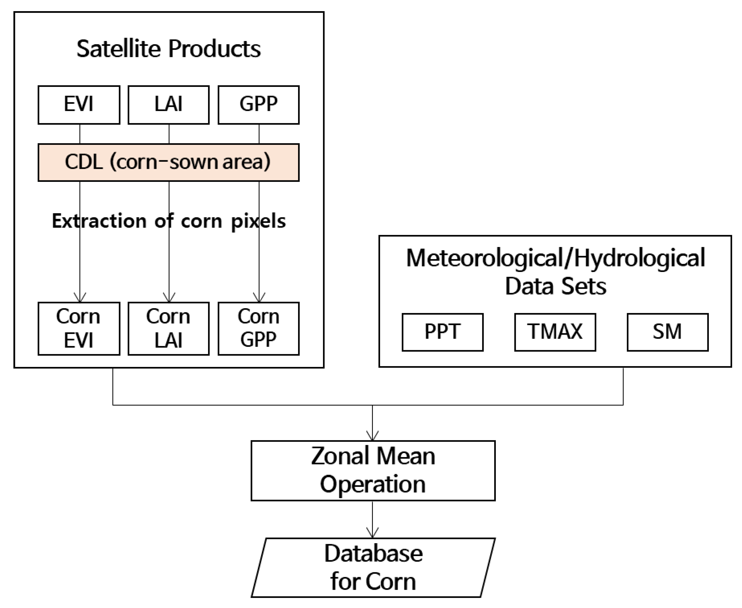
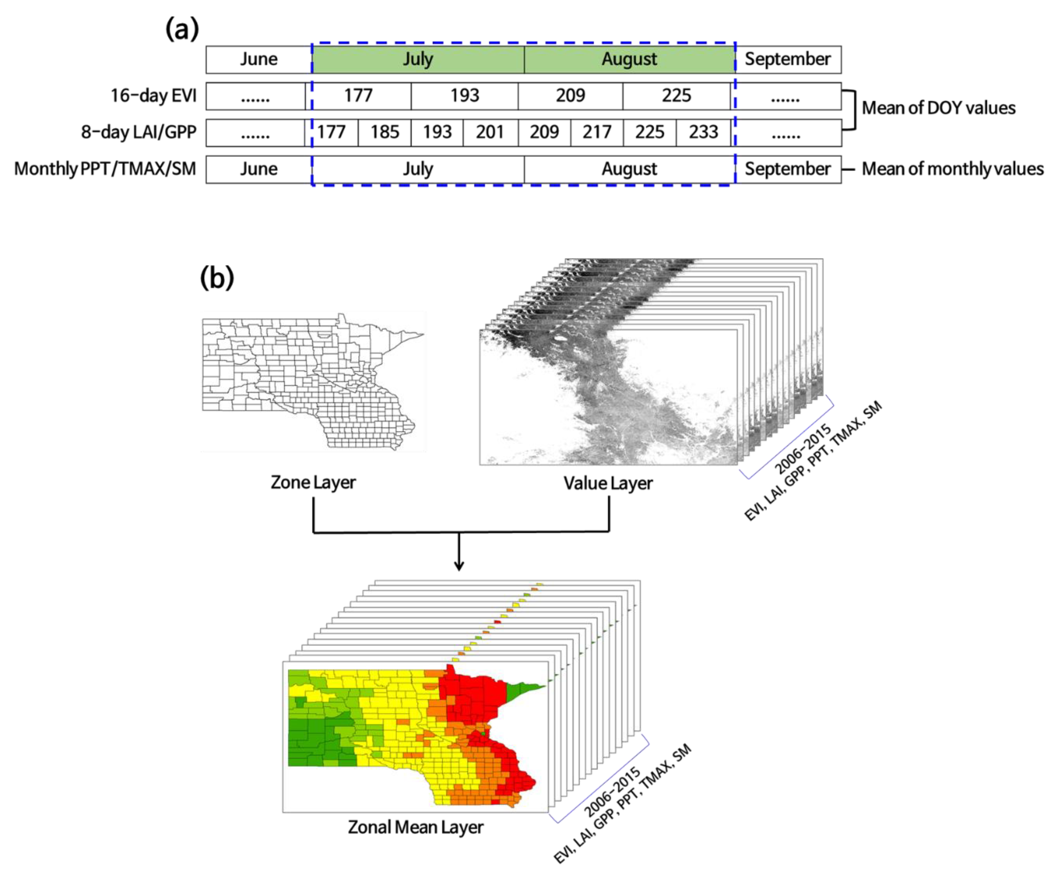
All the data for the period of July and August 2006–2015 are summarized in Table 1. We used cropland data layer (CDL), enhanced vegetation index (EVI), leaf area index (LAI), gross primary production (GPP), precipitation (PPT), maximum temperature (TMAX), and soil moisture (SM) for corn yield prediction. We constructed a spatiotemporal match-up database for corn-sown areas of the Midwestern US to combine the input variables and the yield statistics according to year and county (Figure 2). The temporal aggregation for July–August was conducted for EVI, LAI, and GPP in terms of the day-of-year (DOY), and for PPT, TMAX, and SM in terms of the month (Figure 3a). For spatial aggregation, we first extracted the corn-sown area from the CDL maps at a 56 m resolution for 2006–2009 and at a 30 m resolution for 2010–2015 on the World Geodetic System 1984 (WGS84) coordinate reference system. Then, we overlaid the EVI at 250 m resolution, LAI and GPP at 500 m resolution, PPT and TMAX at 4 km resolution, and SM at a 25 km resolution on the CDL maps. We derived the intersections between the CDL layer and each of the variable layers, which produced the data layers at 56 m or 30 m resolution according to year. The data layers were aggregated by the boundary of the counties in the study area using a zonal mean operation (Figure 3b).

3. Methods

3.1. Definition of Extreme Weather Events

Drought is a natural disaster that causes water shortage and damages agriculture, leading to adverse economic and societal effects [28,29,30]. It also severely affects crop growth and causes considerable reductions in yield. For example, the 2012 US drought influenced at least 60% of the farms and substantially decreased the yields of corn and soybean nationwide [31].
We referred to the National Oceanic and Atmospheric Administration (NOAA) and the National Center for Atmospheric Research (NCAR) for the criteria of drought conditions. The Vegetation Health Index (VHI) [32] provided by NOAA and the Palmer Drought Severity Index (PDSI) [33] provided by NCAR are the mainly used drought indices. The VHI value 0 represents the worst condition, and the VHI value 100 indicates the best situation in terms of vegetation health. PDSI typically shows a range of −4 to +4, with the negative values for dry state and the positive values for wet state. Table 2 shows that the study area suffered a severe drought in July and August (the dominant growth period for corn) in 2012. The mean VHI value for the study area in 2012 was lower than that of the other nine years, and it corresponded to a drought case according to the criteria of NOAA (VHI < 35). The mean PDSI value also satisfied a drought condition in terms of the requirement of NCAR (PDSI < −2). Hence, we considered the year 2012 as a drought case using both indicators from NOAA and NCAR. Corn yields, PPT, minimum temperature (TMIN), TMAX, mean temperature (TMEAN), VHI, and PDSI in July–August for the period between 2006 and 2015 are summarized in Table 2. The counties with a smaller corn yield accompanied by lower precipitation and higher temperature were observed much more frequently in 2012 than in the other years.
High air temperature also significantly affects crop yield, as grains require certain temperatures during the growing season for healthy development. If high temperatures continue for long periods, the crop harvest may be reduced considerably because of weak growth and fruition. Lee at al. [34] used crop growth models with climate data to examine the effects of high-temperature stress on crops; they found that more than 20% of the cultivated area of North America can experience extremely high-temperature stress due to climate change. Climate change would increase thermal stress and damage to crop yields, ultimately affecting the global food supply [5].
For the criteria of heatwave condition from the viewpoint of agriculture, we referred to the two mainly cited studies by Challinor et al. [35] and by Teixeira et al. [5]. Challinor et al. [35] suggested the Heat Stress Intensity (HSI) index that can express the heat stress during the reproductive phase and the yield damage. The HSI index has four categories: low (<0.05), medium (<0.15), high (<0.30), and very high (>0.30). From our match-up database, only four out of the 3585 records (approximately 0.1%) corresponded to the high or very high category. Alternatively, we decided to adopt the critical temperature suggested by Teixeira et al. [5]. Different crops have different thermal stress tolerance levels, and a heatwave limit temperature of 35 °C has been reported for corn and soybeans [5]. In this study, we defined a heatwave as a period when temperatures exceed 35 °C for three consecutive days during July and August. We conducted sensitivity analyses for the corn yield predictions according to the count of successive heatwave days.

3.2. Artificial Intelligence Models

In this paper, six major AI models were employed for crop yield modeling. As a nonparametric regression method, MARS combines multiple linear regression models to handle the nonlinear relationships between explanatory and response variables. The training data set is grouped by adaptive splines having different slopes, which are smoothly connected using a polynomial function. One can evaluate the suitability of a MARS model using the generalized cross-validation (GCV) score [36].
The SVM performs an optimal grouping of data and builds appropriate regression models for each group [37,38,39]. A kernel function such as polynomial, Gaussian, and sigmoid function can be adopted to derive a maximum marginal hyperplane (MMH), which maximizes the margin between data group boundaries [40,41,42]. We used the Gaussian kernel function in this experiment.
Different from the old classification and regression tree (CART), RF is a kind of ensemble method using bootstrap and bagging approaches [43]. The RF builds many decision trees with slightly different characteristics by extracting random samples from training data. The bootstrap evaluates the suitability of the sample distribution and performs resampling if required. The bagging, which is short for bootstrap aggregating, carries out an aggregation of the decision trees created by the bootstrap to produce a final ensemble model using the average or majority vote [44,45]. We set the number of trees to 500 for the tree-pruning process. The number of variables for use in dividing nodes was set to n/3, where n denotes the input feature number. The out-of-bag error was used for measuring the model suitability in our experiment.
The ERT is similar to the RF but different in that it adopts unpruned decision trees. The ERT divides the nodes at random cutpoints and includes the whole training data without bootstrap [46]. We set the parameters for ERT to the same in the RF model: (1) the attribute number for each node and (2) the minimum sample size for dividing nodes.
The ANN emulates a biological neural network. It has input, hidden, and output layers [47]; the hidden layer consists of multiple neurons for computation in a node-link system [48,49]. The model performance depends on the weighting scheme of the network. The training tolerance is an error size for convergence of the model training; the learning rate is an increment/decrement of the weight during an iteration [49]. We set up three nodes in a hidden layer through the performance tests.
The generic ANN has the problem of local minima, such that an optimization process may stop at a locally optimized state, not reaching a global optimization. Also, the overfitting problem is often found in the classic machine learning methods, such that they tend to fail to handle outliers because of excessive training from the given set of data. The DNN overcame these problems in a more intensive network, where backward and forward optimizations are combined. The vanishing gradient issue in the loss function, which may occur in the back-propagation system, can be resolved by adopting activation functions like a rectified linear unit (ReLU). The L1/L2 regularization for outlier management can make the DNN model have sparsity (L1) and simplicity (L2) by detailed scaling of the weighting scheme of the network. Also, the dropout method capably handles extreme cases through iterative training under handicapped conditions where hidden units are randomly deleted [50]. The previously built weighting scheme in a DNN model can be imported for use in the initial values for another DNN model, which is called pretraining and transfer learning. Fine-tuning enables a more precise optimization of a DNN model by adding extra data for training [51].
In this paper, we configured the six AI models through hyperparameter optimization, and the settings are shown in Table 3. In particular, the optimization procedure for the DNN model is illustrated in Figure 4.

3.3. Training and Validation

We conducted 10 rounds of leave-one-year-out blind tests by dividing the data set into a nine-year training group and a one-year validation group from the entire match-up database (2006–2015). For example, the blind test for round #1 consisted of the validation data from 2006 and the training data from the remaining nine years; the blind test for round #2 consisted of the validation data from 2007 and the training data from the remaining nine years, and so on.

4. Results and Discussion

4.1. Experiments under Drought Conditions

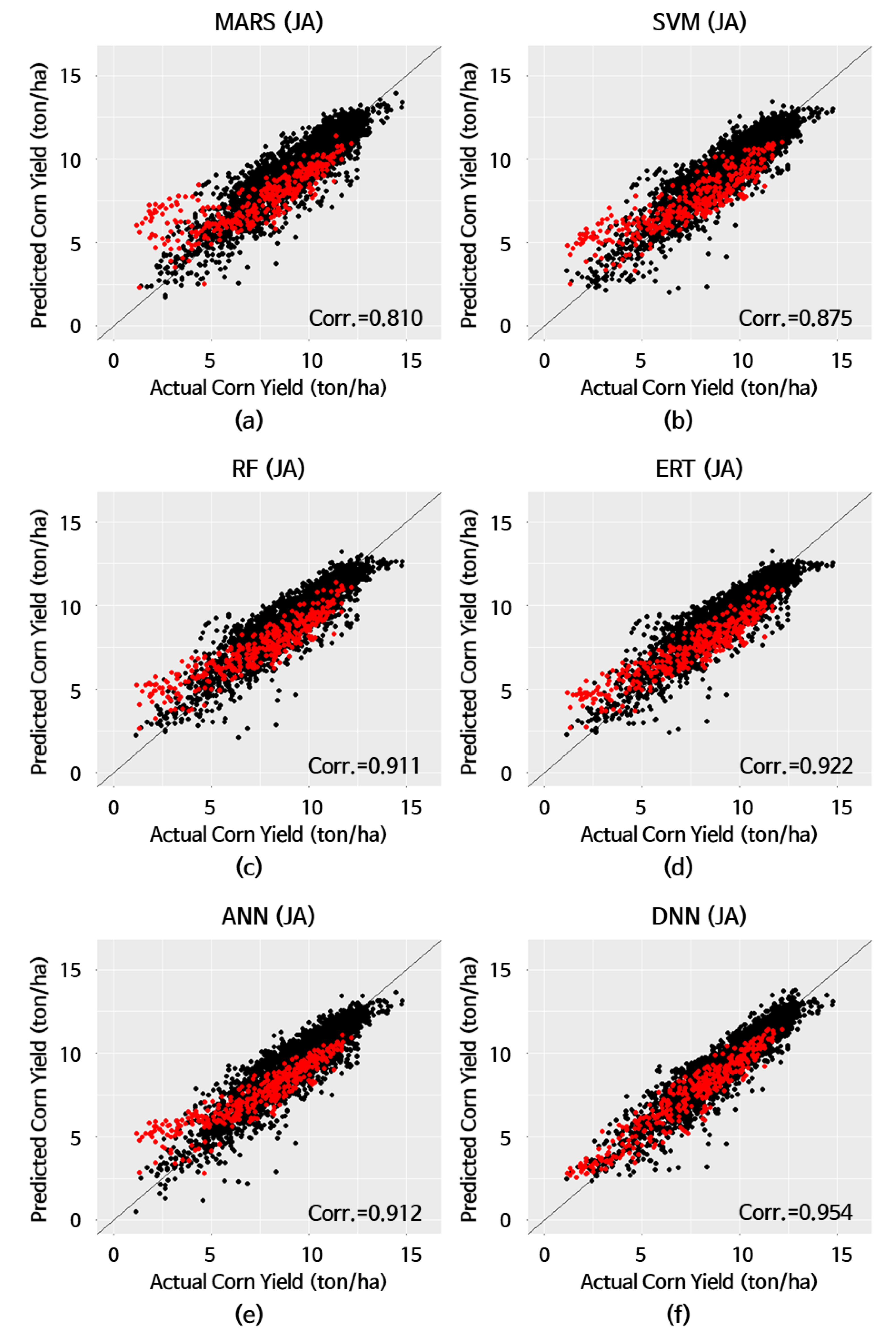
The nationwide drought of the US in 2012 caused severe crop damage, reducing corn yields by about 22.5%. We tested corn yield predictions using the six AI models and the spatiotemporal match-up database to explore how this drought affected the accuracy of yield predictions. Table 4 summarizes the result of the blind test for 2012, in which the nine-year data set (excluding 2012) was used for training, and the data set of 2012 was used for validation. The MARS, SVM, RF, ERT, and ANN models showed the mean absolute error (MAE) between 0.975 and 1.153 ton/ha and the root mean square error (RMSE) between 1.248 and 1.643 ton/ha. In contrast, the DNN model had much lower prediction errors: an MAE of 0.666 ton/ha and an RMSE of 0.828 ton/ha, with 51% (i.e., [1.248 − 0.828]/0.828) to 98% (i.e., [1.643 − 0.828]/0.828) better performance than the other five models in terms of RMSE. The mean absolute percentage error (MAPE) of the DNN model was 12.9%, and the correlation coefficient was 0.954, which can be interpreted as an excellent accuracy even under a natural disaster situation.
Actual and predicted corn yields for the study period are compared in Figure 5, in which red dots indicate 2012 data (severe drought) and black dots indicate all other years. The DNN model resulted in smaller errors and showed more concentration around the 1:1 line. However, the other five models showed more scatter around the 1:1 line and slight overestimation. This overestimation of the other models was because of the failure to cope with the unexpected drought conditions of 2012. Despite the sudden drought, the predicted corn yields of the DNN model were very close to the yield statistics, which indicates that our DNN model successfully overcame the overfitting problem and dealt with outliers appropriately. Maps for actual and predicted corn yields and the prediction errors from the leave-one-year-out blind tests for 2006–2015 are illustrated in Figure 6. The year 2012 for a drought case showed lower corn yields than the other usual years, but the accuracy was similar to that of the other usual years.
Indeed, a larger database can increase the performance and reliability of DNN models. Our database was limited to 10 years because the official maps for crop type were provided since 2006 for our study area. Although the data size was not sufficient, we conducted a sensitivity test according to the size of the training set. We had nine years for the period between 2006 and 2015, except for the year 2012 for a drought case. So, we extracted different combinations of three years (9C3), five years (9C5), and seven years (9C7) from the nine years. As presented in Table 5, 20 experiments for each group were carried out. With the increase in the number of years for training (i.e., 3, 5, 7, and 9), the validation statistics of the DNN model were gradually improved. The RMSE and correlation coefficient showed a slight sensitivity to the volume of training data. However, the accuracy might not offer a dramatic improvement even if the number of years for training surpasses that of our experiment, which should be examined in future work for big data.
In addition to the size of the training dataset, the kinds of input variables can also affect the performance of DNN models. The VHI and the PDSI were used to identify a drought year in our experiment. Here, we incorporated the VHI and the PDSI as an additional input variable for the DNN model. The current model included soil moisture to represent the drought state of cropland. Hence, we examined how the three drought variables (soil moisture, VHI, and PDSI) would influence the performance for prediction. The weights for the three variables connected to the 300-300 hidden units were optimized by the Adaptive Gradient (AdaGrad) algorithm generally used in DNN models. Table 6 shows the validation statistics from the leave-one-year-out blind tests for the year 2012 as a drought case. The model with soil moisture and the model with the addition of VHI and PDSI were compared. The VHI seemed to be appropriate as an additional variable in that the validation statistics showed a slight improvement. On the other hand, the addition of PDSI did not have a critical impact on this experiment. It is partly because the PDSI is an index to represent a climatological drought from the viewpoint of long-term changes, but the VHI is a general indicator of agricultural drought conditions. In addition to the VHI, more input variables that can explain the interactions between climate and vegetation, including evapotranspiration, diurnal temperature change, irrigation capability, and soil properties, will also be necessary for a more reliable prediction of crop yield. Moreover, the appropriate use of drought index will be important for crop yield prediction because a variety of drought indices can represent different aspects of drought conditions.

4.2. Experiments under Heatwave Conditions

Next, we evaluated the accuracy of the AI models for predicting crop yield under heatwave conditions by performing sensitivity analyses for heatwaves of different durations during the study period. We extracted cases in which the counties experienced a heatwave for longer than a given period of days (≥3 to ≥15 days). Then, we calculated validation statistics for these heatwave cases according to the duration of the heatwave using the six AI models for corn yield. As shown in Figure 7, prediction errors tended to increase as the duration of the heatwave increased. However, the accuracy of the DNN model remained significantly stable despite the increase of the heatwave days. In contrast, the errors of the other five models increased somewhat sharply over time. It is interpreted that the DNN model was very robust to unexpected heatwave disasters.
For the heatwaves longer than five and seven days, the average corn yields were 6.628 and 5.938 ton/ha, respectively. Considering that the average corn yield of all the cases was 9.606 ton/ha during the 10 years, it looks like the heatwave significantly damaged the corn yields. Despite the unexpected heatwave disasters, the DNN model showed much lower prediction errors, with the MAE of 0.781 ton/ha for heatwaves exceeding five days, than the other five models having MAE values between 1.068 and 1.352 ton/ha (Table 7). The RMSE of the DNN model was 1.033 ton/ha while the RMSE of the other five models ranged from 1.345 to 1.776 ton/ha, which corresponded to 30% (i.e., [1.345 − 1.033]/1.033) to 72% (i.e., [1.776 − 1.033]/1.033) higher accuracy than the other five models in terms of RMSE. Similarly, for heatwaves longer than seven days, the DNN model outperformed the other five models by approximately 31% to 77% in terms of RMSE (Table 7).
The correlation coefficients of the DNN model were 0.914 and 0.887 for heatwaves longer than five and seven days, respectively, which indicates an excellent agreement with the actual yields under unexpected extreme weather conditions (Figure 8 and Figure 9). The remaining five models showed more deviation from the 1:1 line and significant overestimation. Similar to the drought prediction results, the other five models were unable to deal with the unexpected heatwave cases. However, the corn yields predicted by our DNN model were very close to the actual corn yields, which indicates that this model was constructed appropriately for such extreme weather events. In Figure 10, the Illinois counties outlined in black correspond to the case of heatwaves for more than five consecutive days. The map shows that the counties under heatwave conditions had lower corn yields than the other counties, but the predicted yields were very closely simulated to the actual yields.

4.3. Another Type of Blind Test

An additional experiment was conducted to test the reliability of our approach more objectively. In addition to the leave-one-year-out blind tests in Section 4.1 and Section 4.2, we carried out another type of blind test using the 10-fold cross-validation with random sampling (Figure 11). We rebuilt a DNN model and calibrated the hyperparameters for a new testing environment. As a result, the 10-fold blind tests showed similar validation statistics to those of the leave-one-year-out blind tests, which means that the DNN model was appropriately optimized for corn yield prediction and offered a nice performance for both experiments (Table 8).

5. Conclusions

In this study, we tested six AI models for corn yield under extreme weather conditions and analyzed their performances for a 10-year period that included severe drought and heatwave. Given its tall canopy and broad leaves, corn is relatively sensitive to heat stress [52,53]. In 2012, the Midwestern US experienced severe drought, leading to a 22% reduction in average corn yield. Our DNN model predicted the reduced corn yields in 2012 under drought conditions with a correlation coefficient of 0.954 in the blind tests, which indicates the suitability of our approach for crop yield prediction under extreme weather conditions. Corn yield was remarkably decreased according to the increase of the heatwave duration. Despite the unexpected heatwave, our DNN model produced stable estimates as a result of the effective optimization of hyperparameters, including hidden units, epoch number, activation function, optimizer, L1/L2 regularization, and dropout ratio. Future work using a larger database for about 20 years will be necessary to ensure more reliability of the DNN model for crop yield prediction. Also, more appropriate use of drought index will be required for the prediction of crop yields because various drought indices can represent different aspects of drought conditions.
Losses in crop yield are dependent on the types of extreme weather and the types of crops. For example, the soybean yield is significantly reduced by low temperatures during the growing season [54,55]. Hence, it is also necessary to examine how the crops such as soybean, wheat, and rice are affected by extreme weather conditions, including drought, heat and cold waves, and heavy rainfall. Future studies should use AI modeling to predict the yields of various crops under extreme weather conditions.

Author Contributions

Research design, Y.-W.L.; data analysis, N.K.; manuscript writing, N.K. and Y.-W.L.; literature review and discussion, S.-I.N., C.-W.P., M.H., J.O., K.-J.H., and J.C. All authors have read and agreed to the published version of the manuscript.

Funding

This research was funded by the NRF (National Research Foundation) of the Korean government (2018R1A6A3A01013215 and 2018R1D1A1B07050194). Also, this work was carried out with the support of the “Cooperative Research Program for Agriculture Science & Technology Development (PJ014787042020)”, Rural Development Administration, Republic of Korea.

Conflicts of Interest

The authors declare no conflict of interest.

References

  1. Intergovernmental Panel on Climate Change (IPCC). Climate Change 2014: Impacts, Adaptation and Vulnerability, Part A: Global and Sectoral Aspects, Contribution of Working Group II to the Fifth Assessment Report of the Intergovernmental Panel on Climate Change; Field, C.B., Barros, V.R., Dokken, D.J., Mach, K.J., Mastrandrea, M.D., Bilir, T.E., Chatterjee, M., Ebi, K.L., Estrada, Y.O., Genova, R.C., Eds.; Cambridge University Press: Cambridge, UK; New York, NY, USA, 2014.
  2. Food and Agriculture Organization of the United Nations (FAO). Available online: http://www.fao.org/news/story/tr/item/44570/icode/en/ (accessed on 1 May 2020).
  3. National Oceanic and Atmospheric Administration (NOAA) National Climatic Data Center. Available online: http://www.ncdc.noaa.gov/sotc/hazards/2010/7 (accessed on 1 May 2020).
  4. Lesk, C.; Rowhani, P.; Ramankutty, N. Influence of extreme weather disasters on global crop production. Nature 2016, 529, 84–87. [Google Scholar]
  5. Teixeira, E.I.; Fischer, G.; Van Velthuizen, H.; Walter, C.; Ewert, F. Global hot-spots of heat stress on agricultural crops due to climate change. Agric. Meteorol. 2013, 170, 206–215. [Google Scholar]
  6. Iizumi, T.; Shin, Y.; Kim, W.; Kim, M.; Choi, J. Global crop yield forecasting using seasonal climate information from a multi-model ensemble. Clim. Serv. 2018, 11, 13–23. [Google Scholar] [CrossRef]
  7. Lobell, D.B.; Schlenker, W.; Costa-Roberts, J. Climate trends and global crop production since 1980. Science 2011, 333, 616–620. [Google Scholar] [CrossRef] [Green Version]
  8. Qian, B.; Zhang, X.; Smith, W.; Grant, B.; Jing, Q.; Cannon, A.J.; Neilsen, D.; McConkey, B.; Li, G.; Bonsal, B.; et al. Climate change impacts on Canadian yields of spring wheat, canola and maize for global warming levels of 1.5 °C, 2.0 °C, 2.5 °C and 3.0 °C. Environ. Res. Lett. 2019, 14, 074005. [Google Scholar]
  9. Jeong, J.H.; Resop, J.P.; Mueller, N.D.; Fleisher, D.H.; Yun, K.; Butler, E.E.; Timlin, D.J.; Shim, K.-M.; Gerber, J.S.; eddy, V.R.; et al. Random forests for global and regional crop yield predictions. PLoS ONE 2016, 11, e0156571. [Google Scholar]
  10. Kuwata, K.; Shibasaki, R. Estimating crop yields with deep learning and remotely sensed data. In Proceedings of the 2015 IEEE International Geoscience and Remote Sensing Symposium (IGARSS), Milan, Italy, 26–31 July 2015; pp. 858–861. [Google Scholar]
  11. Kuwata, K.; Shibasaki, R. Estimating corn yield in the United Sates with MODIS EVI and machine learning methods. ISPRS Ann. Photogramm. Remote Sens. Spat. Inf. Sci. 2016, 3, 131–136. [Google Scholar]
  12. Kim, N.; Ha, K.-J.; Park, N.-W.; Cho, J.; Hong, S.; Lee, Y.-W. A comparison between major artificial intelligence models for crop yield prediction: Case study of the Midwestern United States, 2006–2015. ISPRS Int. J. Geo Inf. 2019, 8, 240. [Google Scholar]
  13. Taylor, R.D.; Koo, W.W. Outlook of the U.S. and world corn and soybean industries, 2010–2020. In Agribusiness and Applied Economics Report; North Dakota State University: Fargo, ND, USA, 2011; p. 682. [Google Scholar]
  14. Food and Agriculture Organization of the United Nations (FAO). FAO Statistical Databases. 2013. Available online: http://faostat.fao.org (accessed on 1 March 2020).
  15. NASA EARTHDATA Search Home Page. Available online: https://search.earthdata.nasa.gov/ (accessed on 1 March 2020).
  16. Townshend, J.R.G.; Justice, C.O.; Li, W.; Gurney, C.; McManus, J. Global land cover classification by remote sensing: Present capabilities and future capabilities. Remote Sens. Environ. 1991, 35, 243–255. [Google Scholar]
  17. Huete, A.R.; Didan, K.; Miura, T.; Rodriguez, E.P.; Gao, X.; Ferreria, L.G. Overview of the radiometric and biophysical performance of the MODIS vegetation indices. Remote Sens. Environ. 2002, 83, 195–213. [Google Scholar] [CrossRef]
  18. Sellers, P.J. Canopy reflectance, photosynthesis and transpiration. Int. J. Remote Sens. 1985, 6, 1335–1372. [Google Scholar] [CrossRef]
  19. Lee, S.-J.; Cho, J.; Hong, S.; Ha, K.-J.; Lee, H.; Lee, Y.-W. On the relationships between satellite-based drought index and gross primary production in the North Korean croplands, 2000–2012. Remote Sens. Lett. 2016, 7, 790–799. [Google Scholar] [CrossRef]
  20. PRISM Climate Group Home Page. Available online: http://www.prism.oregonstate.edu/ (accessed on 1 March 2020).
  21. GES DISC Home Page. Available online: https://disc.gsfc.nasa.gov/ (accessed on 1 March 2020).
  22. Rodell, M.; Houser, P.R.; Jambor, U.; Gottschalck, J.; Mitchell, K.; Meng, C.-J.; Arsenault, K.; Cosgrove, B.; Radakovich, J.; Bosilovich, M.; et al. The global land data assimilation system. Bull. Am. Meteorol. Soc. 2004, 85, 381–394. [Google Scholar] [CrossRef] [Green Version]
  23. De Jeu, R.; Holmes, T.; Dorigo, W.; Wagner, W.; Hahn, S.; Parinussa, R. Evaluation of SMOS soil moisture with other existing satellite products. In Proceedings of the Remote Sensing and Hydrology 2010 Symposium, Jackson Hole, WY, USA, 27–30 September 2010. [Google Scholar]
  24. NASS USDA Home Page. Available online: https://www.nass.usda.gov/ (accessed on 1 March 2020).
  25. Boryan, C.; Yang, Z.; Mueller, R.; Craig, M. Monitoring US agriculture: The US department of agriculture, national agricultural statistics service, cropland data layer program. Geocarto Int. 2011, 26, 341–358. [Google Scholar] [CrossRef]
  26. Becker-Reshef, I.; Vermote, E.; Lindeman, M.; Justice, C. A generalized regression-based model for forecasting winter wheat yields in Kansas and Ukraine using MODIS data. Remote Sens. Environ. 2010, 114, 1312–1323. [Google Scholar] [CrossRef]
  27. NASS USDA Quick Stats Home Page. Available online: http://quickstats.nass.usda.gov (accessed on 1 March 2020).
  28. Wilhite, D.A.; Glantz, M.H. Understanding: The drought phenomenon: The role of definitions. Water Int. 1985, 10, 111–120. [Google Scholar] [CrossRef] [Green Version]
  29. Quiring, S.M.; Papakryiakou, T.N. An evaluation of agricultural drought indices for the Canadian prairies. Agric. For. Meteorol. 2003, 118, 49–62. [Google Scholar] [CrossRef]
  30. Vicente-Serrano, S.M.; Gouveia, C.; Camarero, J.J.; Beguería, S.; Trigo, R.; López-Moreno, J.I.; Azorín-Molina, C.; Pasho, E.; Lorenzo-Lacruz, J.; Revuelto, J.; et al. Response of Vegetation to Drought Time-Scales across Global Land Biomes. Proc. Natl. Acad. Sci. USA 2013, 110, 52–57. [Google Scholar] [CrossRef] [Green Version]
  31. Crutchfiled, S.U.S. Drought 2012: Farm and Food Impacts; USDA Economic Research Service: Washington, DC, USA, 2012.
  32. Global Vegetation Health Products. Available online: https://www.star.nesdis.noaa.gov/smcd/emb/vci/VH/index.php (accessed on 18 May 2020).
  33. Palmer Drought Severity Index (PDSI). Available online: https://climatedataguide.ucar.edu/climate-data/palmer-drought-severity-index-pdsi (accessed on 18 May 2020).
  34. Lee, K.; Kang, H.-S.; Cho, C.H. Climate change-induced high temperature stress on global crop production. Korean Geogr. Soc. 2016, 51, 622–649. [Google Scholar]
  35. Challinor, A.J.; Wheeler, T.R.; Craufurd, P.Q.; Slingo, J.M. Simulation of the impact of high temperature stress on annual crop yields. Agric. Meteorol. 2005, 135, 180–189. [Google Scholar] [CrossRef] [Green Version]
  36. Hastie, T.; Tibshirani, R.; Friedman, J. The Elements of Statistical Learning: Data Mining, Inference and Prediction, 2nd ed.; Springer: New York, NY, USA, 2009. [Google Scholar]
  37. Pal, M.; Mather, P.M. An assessment of the effectiveness of decision tree methods for land cover classification. Remote Sens. Environ. 2003, 86, 554–565. [Google Scholar]
  38. Jensen, J.R.; Im, J.; Hardin, P.; Jense, R.R. Image Classification. In The Sage Handbook of Remote Sensing; Warner, T.A., Nellis, M.D., Foody, G.M., Eds.; SAGE Publications Ltd.: London, UK, 2009; Chapter 19; pp. 269–296. [Google Scholar]
  39. Duro, D.C.; Franklin, S.E.; Dube, M.G. A comparison of pixel-based and object-based image analysis with selected machine learning algorithms for the classification of agricultural landscapes using SPOT-5 HRG imagery. Remote Sens. Environ. 2012, 118, 259–272. [Google Scholar] [CrossRef]
  40. Mountrakis, G.; Im, J.; Ogole, C. Support vector machines in remote sensing: A review. ISPRS J. Photogramm. Remote Sens. 2011, 66, 247–259. [Google Scholar] [CrossRef]
  41. Foody, G.M.; Mathur, A. The use of small training sets containing mixed pixels for accurate hard image classification: Training on mixed spectral responses for classification by SVM. Remote Sens. Environ. 2006, 103, 179–189. [Google Scholar]
  42. Van der Linder, S.; Hoster, P. The influence of urban structures on impervious surface maps from airborne hyperspectral data. Remote Sens. Environ. 2009, 113, 2298–2305. [Google Scholar] [CrossRef]
  43. Breiman, L.; Culter, A. Random Forests. 2014. Available online: http://www.stat.berkeley.edu/~breiman/RandomForests/cc_home.htm (accessed on 1 March 2020).
  44. Breiman, L. Random forests. Mach. Learn. 2001, 45, 5–32. [Google Scholar] [CrossRef] [Green Version]
  45. Ali, J.; Khan, R.; Ahmad, N.; Maqsood, I. Random forests and decision trees. Int. J. Comput. Sci. Issues 2012, 9, 272–278. [Google Scholar]
  46. Geurts, P.; Ernst, D.; Wehenkel, L. Extremely randomized trees. Mach. Learn. 2006, 63, 3–42. [Google Scholar]
  47. Kaul, M.; Hill, R.L.; Walthall, C. Artificial neural networks for corn and soybean yield prediction. Agric. Syst. 2005, 85, 1–18. [Google Scholar]
  48. Brown, M.E.; Lary, D.J.; Vrieling, A.; Stathakis, D.; Mussan, H. Neural networks as a tool for constructing continuous NDVI time series from AVHRR and MODIS. Int. J. Remote Sens. 2008, 29, 7141–7158. [Google Scholar] [CrossRef] [Green Version]
  49. Ji, B.; Sun, Y.; Yang, S.; Wan, J. Artificial neural networks for rice yield prediction in mountainous regions. J. Agric. Sci. 2007, 145, 249–261. [Google Scholar] [CrossRef]
  50. Pham, V.; Bluche, T.; Kernorvant, C.; Louradour, J. Drop-out improves recurrent neural networks for handwriting recognition. In Proceedings of the 2014 14th International Conference on Frontiers in Handwriting Recognition (ICFHR), Crete, Greece, 1–4 September 2014. [Google Scholar]
  51. Erhan, D.; Bengio, Y.; Courville, A.; Manzagol, P.A.; Vincent, P. Why does unsupervised pre-training help deep learning? J. Mach. Learn. Res. 2010, 11, 625–660. [Google Scholar]
  52. Classen, M.M.; Shaw, R.H. Water deficit effects on corn. I. Grain components. Agron. J. 1970, 62, 652–655. [Google Scholar] [CrossRef]
  53. Carlson, R.E. Heat stress, plant-available soil moisture, and corn yields in Iowa: A short- and long-term view. J. Prod. Agric. 2013, 3, 293–297. [Google Scholar]
  54. Thomas, J.F.; Raper, C.D.; Weeks, W.W. Day and night temperature effects on nitrogen and soluble carbohydrate allocation during early reproductive growth in soybeans. Agron. J. 1981, 73, 577–582. [Google Scholar] [CrossRef]
  55. Wallace, D.H. Physiological genetics of plant maturity, adaptation, and yield. In Plant Breeding Review; Janick, J., Ed.; John Wiley & Sons, Inc.: Hoboken, NJ, USA, 1985; Volume 3, pp. 21–167. [Google Scholar]
Figure 1. Study area.
Applsci 10 03785 g001
Figure 2. Process for constructing the match-up database for corn yield for the counties of the study area.
Applsci 10 03785 g002
Figure 3. Concept of the (a) temporal aggregation for July–August and the (b) spatial aggregation using zonal mean operation for the counties of the study area.
Applsci 10 03785 g003
Figure 4. Hyperparameter optimization for the deep neural network (DNN) model of this study.
Applsci 10 03785 g004
Figure 5. Actual and predicted corn yields for 2006–2015. Red dots, 2012 data under drought conditions; black dots, all other years. (a) Multivariate adaptive regression spline (MARS); (b) Support vector machine (SVM); (c) Random forest (RF); (d) Extremely randomized tree (ERT); (e) Artificial neural network (ANN); (f) Deep neural network (DNN).
Applsci 10 03785 g005
Figure 6. Maps for (a) actual and (b) predicted corn yields and the (c) prediction errors from the leave-one-year-out blind tests for 2006–2015. The year 2012 for a drought case showed lower corn yields than the other typical years, but the accuracy was similar to that of the other years.
Applsci 10 03785 g006
Figure 7. Validation statistics for prediction of corn yield during heatwave obtained from leave-one-year-out experiments for 2006–2015. (a) Mean absolute percentage error (MAPE); (b) Root mean square error (RMSE).
Applsci 10 03785 g007
Figure 8. Actual and predicted corn yields from the leave-one-year-out blind tests for 2006–2015: Red dots, heatwave exceeding five days; black dots, all other cases. (a) Multivariate adaptive regression spline (MARS); (b) Support vector machine (SVM); (c) Random forest (RF); (d) Extremely randomized tree (ERT); (e) Artificial neural network (ANN); (f) Deep neural network (DNN).
Applsci 10 03785 g008
Figure 9. Actual and predicted corn yields from the leave-one-year-out blind tests for 2006–2015: Red dots, heatwave exceeding seven days; black dots, all other cases. (a) Multivariate adaptive regression spline (MARS); (b) Support vector machine (SVM); (c) Random forest (RF); (d) Extremely randomized tree (ERT); (e) Artificial neural network (ANN); (f) Deep neural network (DNN).
Applsci 10 03785 g009
Figure 10. Maps of (a) actual and (b) predicted corn yields from the leave-one-year-out blind tests for 2007. The Illinois counties outlined in black were affected by the heatwaves for longer than five consecutive days.
Applsci 10 03785 g010
Figure 11. Concept of 10-fold cross-validation with random sampling for the blind tests of corn yield prediction during 2006–2015.
Applsci 10 03785 g011
Table 1. The data used for corn yield prediction.
DataSpatial ResolutionTemporal ResolutionSource
CroplandCDL (1)56 m (2006–2009)
30 m (2010–2015)
YearlyUSDA (8)
Satellite imagesEVI (2)250 m16 daysNASA EOSDIS (9)
LAI (3)500 m8 days
GPP (4)
Meteorological dataPPT (5)4 kmMonthlyPRISM (10) Climate Group
TMAX (6)
Hydrological dataSM (7)25 kmMonthlyNASA GES DISC (11)
Yield statisticsCornCountyYearlyUSDA (8)
(1) Cropland Data Layer; (2) Enhanced Vegetation Index; (3) Leaf Area Index; (4) Gross Primary Production; (5) Precipitation; (6) Maximum air temperature; (7) Soil Moisture; (8) United States Department of Agriculture; (9) National Aeronautics and Space Administration’s Earth Observing System Data and Information System; (10) Parameter-elevation Regressions on Independent Slopes Model; (11) NASA’s Goddard Earth Sciences Data and Information Services Center.
Table 2. Annual corn yield and the precipitation (PPT), minimum air temperature (TMIN), maximum air temperature (TMAX), mean air temperature (TMEAN), Vegetation Health Index (VHI), and Palmer Drought Severity Index (PDSI) for July and August in the study area.
YearCorn Yield (ton/ha)PPT (mm/Month)TMIN (°C)TMAX (°C)TMEAN (°C)VHI (0 to 100)PDSI (Unitless)
20068.51985.617.029.823.445.2−0.886
20078.871103.516.629.122.849.01.083
20089.42083.815.628.321.958.02.855
200910.061105.414.326.020.168.72.890
20109.167119.517.429.323.361.14.953
20118.93882.917.629.623.661.33.288
20127.35252.916.630.923.732.2 (1)−3.336 (2)
20139.48952.115.728.021.958.5−0.207
201410.26599.515.526.721.170.11.149
201510.651112.115.627.321.565.01.066
Mean9.28389.716.228.522.356.91.286
(1) belongs to drought condition in terms of the criteria of National Oceanic and Atmospheric Administration (VHI < 35); (2) belongs to drought condition in terms of the criteria of National Center for Atmospheric Research (PDSI < −2).
Table 3. Hyperparameters and libraries used for the six AI models in this study.
ModelHyperparameters (Optimized)Library Used
MARS (1)Pruning method: backwardearth library in R
SVM (2)Kernel function: Gaussian radial basis functione1071 library in R
RF (3)Number of trees: 500
Number of variables used for splitting nodes: n/3
(n is the number of input variables)
randomForest library in R
ERT (4)Number of trees: 500
Number of variables used for splitting nodes: n/3
(n is the number of input variables)
extraTrees library in R
ANN (5)Number of hidden units: 3nnet library in R
DNN (6)Hidden units: 300–300
Loss function: Sum of Squared Errors (SSE)
Activation function: Rectified Linear Unit (ReLU)
Optimizer: Adaptive Gradient (AdaGrad)
Dropout ratio: 40%
tensorflow library in Python
(1) Multivariate Adaptive Regression Splines; (2) Support Vector Machine; (3) Random Forest; (4) Extremely Randomized Trees; (5) Artificial Neural Network; (6) Deep Neural Network.
Table 4. Summary of validation statistics for prediction of corn yield in 2012 as a drought case.
ModelMBE (1) (ton/ha)MAE (2) (ton/ha)RMSE (3) (ton/ha)MAPE (4) (%)Corr.(5)
MARS (6)0.1681.1531.64329.20.810
SVM (7)0.0191.1231.42325.00.875
RF (8)0.0681.0251.30323.20.911
ERT (9)−0.0561.0121.24821.60.922
ANN (10)0.1710.9751.30423.70.912
DNN (11)−0.0170.6660.82812.90.954
(1) Mean Bias Error; (2) Mean Absolute Error; (3) Root Mean Square Error; (4) Mean Absolute Percentage Error; (5) Correlation Coefficient; (6) Multivariate Adaptive Regression Splines; (7) Support Vector Machine; (8) Random Forest; (9) Extremely Randomized Trees; (10) Artificial Neural Network; (11) Deep Neural Network.
Table 5. Summary of validation statistics according to the number of years used in training for prediction of corn yield in 2012 as a drought case.
No. of Years for TrainingNo. of Experiments (1)MBE (2) (ton/ha)MAE (3) (ton/ha)RMSE (4) (ton/ha)MAPE (5) (%)Corr.(6)
3 years20 out of 9C30.0700.9201.15419.00.919
5 years20 out of 9C5−0.0910.9151.15319.10.926
7 years20 out of 9C70.0070.8741.09018.20.931
9 years1 (9C9)−0.0170.6660.82812.90.954
(1) Randomly chosen from the whole combinations; (2) Mean Bias Error; (3) Mean Absolute Error; (4) Root Mean Square Error; (5) Mean Absolute Percentage Error; (6) Correlation Coefficient.
Table 6. Summary of validation statistics according to the addition of drought-related variables for prediction of corn yield in 2012 as a drought case.
ModelsMBE (1) (ton/ha)MAE (2) (ton/ha)RMSE (3) (ton/ha)MAPE (4) (%)Corr.(5)
Current model (w/ SM (6))−0.0170.6660.82812.90.954
Current model (w/ SM) + VHI (7)−0.0380.6180.79111.40.954
Current model (w/ SM) + PDSI (8)−0.0210.7040.91412.50.937
Current model (w/ SM) + VHI + PDSI0.0130.6320.81811.40.950
(1) Mean Bias Error; (2) Mean Absolute Error; (3) Root Mean Square Error; (4) Mean Absolute Percentage Error; (5) Correlation Coefficient; (6) Soil Moisture; (7) Vegetation Health Index; (8) Palmer Drought Severity Index.
Table 7. Summary of validation statistics for prediction of corn yield during heatwaves longer than five and seven consecutive days obtained from leave-one-year-out blind tests for 2006–2015.
ModelMBE (1) (ton/ha)MAE (2) (ton/ha)RMSE (3) (ton/ha)MAPE (4) (%)Corr.(5)
HW5 (6)MARS (8)0.4901.3521.77632.30.748
SVM (9)0.3281.1801.51026.60.816
RF (10)0.3261.1041.41125.10.840
ERT (11)0.2571.0681.34523.60.853
ANN (12)0.3501.1191.45926.00.830
DNN (13)0.1080.7811.03315.80.914
HW7(7)MARS (8)
SVM (9)
0.546
0.445
1.514
1.278
1.974
1.638
40.9
33.1
0.622
0.755
RF (10)
ERT(11)
0.401
0.307
1.220
1.165
1.550
1.463
31.2
28.9
0.785
0.808
ANN (12)
DNN (13)
0.414
0.101
1.263
0.857
1.626
1.117
32.9
18.9
0.757
0.887
(1) Mean Bias Error; (2) Mean Absolute Error; (3) Root Mean Square Error; (4) Mean Absolute Percentage Error; (5) Correlation Coefficient; (6) heatwaves longer than five consecutive days; (7) heatwaves longer than seven consecutive days; (8) Multivariate Adaptive Regression Splines; (9) Support Vector Machine; (10) Random Forest; (11) Extremely Randomized Trees; (12) Artificial Neural Network; (13) Deep Neural Network.
Table 8. Summary of comparisons between leave-one-year-out and 10-fold blind tests for the deep neural network models for prediction of corn yield under drought and heatwave conditions during 2006–2015.
Validation MethodMBE (1)
(ton/ha)
MAE (2)
(ton/ha)
RMSE (3)
(ton/ha)
MAPE (4)
(%)
Corr.(5)
Droughtleave-one-year-out−0.0170.6660.82812.90.954
10-fold−0.0010.6940.93412.60.934
HW ≧ 5 (6)leave-one-year-out0.1080.7811.03315.80.914
10-fold0.0190.7801.07915.90.906
HW ≧ 7 (7)leave-one-year-out0.1010.8571.11718.90.887
10-fold0.0830.8631.17919.00.875
(1) Mean Bias Error; (2) Mean Absolute Error; (3) Root Mean Square Error; (4) Mean Absolute Percentage Error; (5) Correlation Coefficient; (6) heatwaves longer than five consecutive days; (7) heatwaves longer than seven consecutive days.