Article

Deformation of Air Bubbles Near a Plunging Jet Using a Machine Learning Approach

1
National Research Council, Institute of Marine Engineering, Via di Vallerano, 139-00128 Roma, Italy
2
Department of Civil and Mechanical Engineering, University of Cassino and Southern Lazio, Via G. Di Biasio, 43-03043 Cassino (FR), Italy
*
Author to whom correspondence should be addressed.
Appl. Sci. 2020, 10(11), 3879; https://doi.org/10.3390/app10113879
Submission received: 9 May 2020 / Revised: 26 May 2020 / Accepted: 1 June 2020 / Published: 3 June 2020
(This article belongs to the Special Issue Machine Learning Algorithms for Hydraulic Engineering)

Abstract

:
The deformation of air bubbles in a liquid flow field is of relevant interest in phenomena such as cavitation, air entrainment, and foaming. In complex situations, this problem cannot be addressed theoretically, while the accuracy of an approach based on Computational Fluid Dynamics (CFD) is often unsatisfactory. In this study, a novel approach to the problem is proposed, based on the combined use of a shadowgraph technique, to obtain experimental data, and some machine learning algorithms to build prediction models. Three models were developed to predict the equivalent diameter and aspect ratio of air bubbles moving near a plunging jet. The models were different in terms of their input variables. Five variants of each model were built, changing the implemented machine learning algorithm: Additive Regression of Decision Stump, Bagging, K-Star, Random Forest and Support Vector Regression. In relation to the prediction of the equivalent diameter, two models provided satisfactory predictions, assessed on the basis of four different evaluation metrics. The third model was slightly less accurate in all its variants. Regarding the forecast of the bubble’s aspect ratio, the difference in the input variables of the prediction models shows a greater influence on the accuracy of the results. However, the proposed approach proves to be promising to address complex problems in the study of multi-phase flows.

1. Introduction

The study of the dynamics of air bubbles in a liquid flow field is of practical interest in many areas of environmental, chemical, naval and ocean engineering. The interest in phenomena such as cavitation, air entrainment and foaming is particularly relevant. The theoretical characterization of motion and deformation of isolated bubbles is effective only in simple special cases. The most basic theoretical model of the dynamics of a single bubble is represented by the Rayleigh–Plesset equation [1,2], which allows for a description of the variation in the bubble radius as a function of four forcers: the external pressure, the internal pressure of the bubble, the surface tension of the liquid and the viscosity of the liquid. It is valid in the case of a perfectly spherical bubble in an infinite liquid domain that is at rest far from the bubble. Moreover, temperature gradients are not considered, while the pressure is a known input governing the bubble deformation. In most situations of practical interest, these assumptions cannot be justified. Later, various authors proposed other theoretical models under different hypotheses [3,4,5,6].
More complex situations are generally modelled by experimental [7,8,9,10] or CFD-based approaches [11,12,13,14].
However, the dynamics of individual bubbles in a water volume are governed by the physical characteristics of water and air, which can be expressed in terms of water density ρw, bubble density ρb, water dynamic viscosity μ and water surface tension σ. The rising of an air bubble depends also on the buoyancy, which is a function of the pressure gradient ∂P/∂z, where z indicates the water depth, and that of the gravitational acceleration g. The buoyancy also depends on the air bubble volume, related to the bubble equivalent diameter (Deq) (i.e., the diameter of a sphere of volume equal to the bubble volume). Furthermore, the relative motion between the air bubble and the surrounding water, which moves with velocity Vw, involves a resistance related to the bubble velocity Vb [15]. In general, the evolution of a single bubble that moves in the water can be described according to:
f ( ρ w , ρ b , μ , σ , D e q , g , P z , V w , V b ) = 0
Based on the well-known dimensional analysis [16,17,18], four essential dimensionless numbers affecting the evolution of individual bubbles can be obtained:
R e b = V b D e q υ
F r b = V b g D e q
W e b = ρ w V b 2 D e q σ
E o = ( ρ w ρ b ) g D e q 2 σ
where Reb is the bubble Reynolds number, υ is the water cinematic viscosity, Frb is the bubble Froude number, Web is the bubble Weber number and Eo is the Eötvös number.
A somewhat complex phenomenon that induces the movement of bubbles in a water volume is observed in the presence of a plunging jet. When a water jet plunges into a water pool, air bubbles are generally entrained and carried away in the water volume (Figure 1) if the jet impact velocity exceeds a critical value [19]. The impact of the jet induces a fluctuating pressure field that is very difficult to characterize [20]. Moreover, in the turbulent flow induced by the plunging jet, the evolution of the bubbles is also governed by other mechanisms, e.g., turbulence fluctuation, drag, turbulent shear, etc. [21].
The knowledge of the pressure and shear stress is essential to accurately predict the evolution of the size and shape of the bubbles near the plunging jet, since the shape of a single bubble can fluctuate in response to oscillations in the pressure and shear stress in the liquid surrounding the bubble [22,23].
However, even if the pressure field is not known, the availability of a good amount of data on the evolution of the size and shape of a suitable number of bubbles, as well as of data on some characteristics of the flow field, leads us to consider an interesting alternative approach for predicting the deformation of individual bubbles: machine learning algorithms. These procedures, particularly suited to dealing with nonlinear regression problems dependent on several variables, have been widely used in recent years in solving a variety of water engineering problems [24,25,26,27,28,29,30,31,32,33,34].
The complexity of the observed phenomena makes two-phase air–water flows a field of investigation for which machine learning algorithms can represent a very useful tool. However, so far in the literature, there are few studies relating to the application of machine learning algorithms to two-phase air–water flow issues. Shaban and Tavoularis [35] developed a novel method to evaluate gas and liquid flow rates in vertical upward gas–liquid pipe flows. This technique consisted of an application of multi-layer backpropagation neural networks on the probability density function and the power spectral density of the normalized output of a differential pressure transducer connected to two axially separated wall pressure taps in the pipe. Granata and de Marinis [36] used the Regression Tree M5P model, Bagging algorithm and Random Forest algorithm to address some complex problems of wastewater hydraulics, including the air entrainment in a circular drop manhole under supercritical flow. Mosavi et al. [37] used an adaptive network-based fuzzy inference system (ANFIS) combined with CFD data to predict the macroscopic parameters such as gas velocity in the multiphase reactor. The mentioned studies already show the remarkable potential of approaches based on machine learning algorithms in addressing issues related to multi-phase flows.
However, to the best of the authors’ knowledge, there are no previous studies based on machine learning algorithms that deal with the evolution of air bubbles in water volume.
In this research, three different data-driven models have been developed for the prediction of bubble equivalent diameter (Deq) and aspect ratio (AR), where AR is equal to the ratio of the minor axis and major axis of the air bubble fitting ellipsoid [38].
The models differ in terms of their input variables. Five variants of each model have been built, varying the used machine learning algorithms, which are Additive Regression of Decision Stumps (ARDS), Bootstrap Aggregating (Bagging), K-Star, Random Forest (RF) and Support Vector Regression (SVR). In general terms, the forecasting capability of different machine learning algorithms is strongly dependent on the size and variety of the available dataset. The abovementioned algorithms have been selected because they usually ensure high performance in modelling complex and highly non-linear relationships. The input parameters of the models have been evaluated through experimental measurements carried out using a shadowgraph technique, which will be described in detail in the following section.

2. Material and Methods

2.1. Experimental Setup

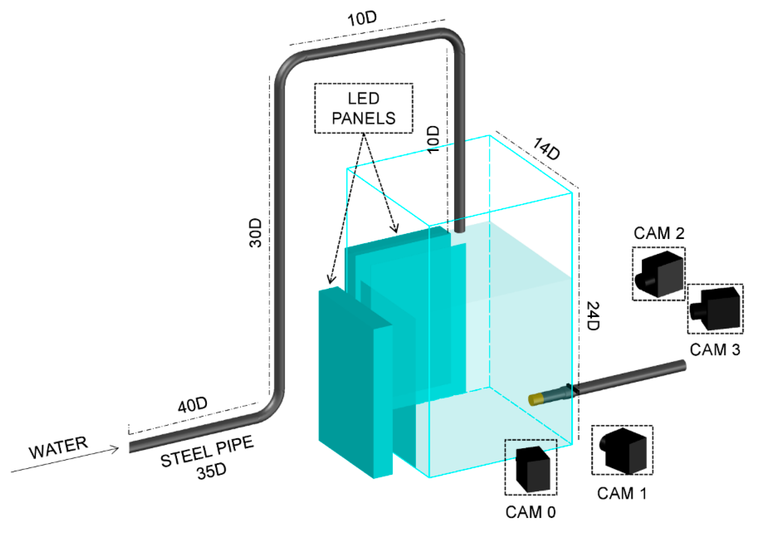
The experimental facility (Figure 2) consists of a vertical steel pipe with nozzle diameter D = 21 mm, from which a vertical plunging jet falls in a Plexiglas prismatic tank with a side equal to 14D and a height equal to 24D. The water flow is recirculated in a closed circuit, supplied by a centrifugal pump. The test water flow rate was Q = 0.5 L/s, measured by means of an electromagnetic flow meter.
The plunging jet axis is in the centerline of the tank with the jet nozzle located at 5D from the free surface and 20D from the bottom of the tank.
The shadowgraph system consists of four Falcon® 1.4MP fast cameras (Teledyne DALSA, Waterloo, ON, Canada), with 35-mm focal length lenses and a resolution of 1400 × 1024 pixels at 100 frames per second. Cameras are arranged in couples and located in front of two different tank sides at a 90° angle. On the opposite tank sides, a couple of LED panels, with a size of 297 × 210 mm and a power of 30 W, were placed for the backlight illumination of the measurement volume. The investigated volume extends from the free surface to 6.5D streamwise (vertical x-direction), from −2.5D to 2.5D spanwise (y-direction) and from −1D to 1D depthwise (z-direction).
An experimental test consisting of 2000 consecutive images has been carried out. In order to evaluate the shape evolution of some air bubbles near the vertical plunging jet, the image sequences have been recorded with a frame rate equal to 100 Hz with an image size of 1400 × 751 pixels and a high spatial resolution, close to 0.1 mm/pixel. It should be noted that an increase in the camera’s frame rate corresponds to a decrease in the image size, leading to a reduction in the investigated volume. Therefore, the frame rate has been optimized to ensure an investigated volume wide enough to allow for an analysis of the rising bubbles inside the lateral recirculation zone.

2.2. Volumetric Shadowgraph Technique

The volumetric shadowgraph technique used in this study allows us to describe the three-dimensional evolution of air bubble shape and position, based on the observation of the bubble boundaries from different points of view [39,40]. The boundary projection in the Euclidean space defines a cone whose axis joins the center of the camera lens to the bubble centroid. This principle is illustrated in Figure 3, considering the projection of an object on two different planes, Oxy and O’x’y’, with the local z-axis indicating the camera’s optical axis.
If the extrinsic and intrinsic parameters of the camera system are known, it is possible to project, in the three-dimensional space, the n cones, with n equal to the number of cameras. The extrinsic parameters define the location and orientation of the camera reference frame with respect to a known world reference frame, while intrinsic parameters define the optical, geometric and digital characteristics of the camera, regardless of the world around it [41,42].
The estimation of the camera parameters takes place through a well-established calibration procedure [43], which involves the use of a specific target, consisting of a planar chessboard 90 × 50 mm with squares of 5 mm ± 0.02 mm in size, stuck on a planar steel plate. The calibration requires the acquisition of a sequence of 40 images containing the entire translated and rotated target. The corner identification in each target image allows us to evaluate the extrinsic parameters of each camera. Then, the evaluation of the relative position and orientation of Cam1 to Cam0 and of Cam3 to Cam2 and the subsequent estimation of the position and orientation of the two camera couples, both relative and absolute, with respect to the world coordinate system, provide the mapping of the target and, consequently, of the investigated volume.
The intersection of the n cones defines the carved hull of the same [44]. Therefore, using sufficiently fast cameras, this technique allows for the detection and description of the spatial and temporal evolution of individual air bubbles within a measurement volume.
A specific image processing algorithm (Figure 4) has been used to detect the air bubble boundaries of each recorded data set. The procedure entails two preliminary steps: the first is the background removal (Figure 4b), obtained by subtracting from each image the median image calculated over the entire data set, the second step is the image binarization (Figure 4c) by means of the IsoData threshold algorithm [45]. The latter allows for the detection of the bubbles characterized by a clearly visible boundary, removing the out-of-focus bubbles. In the presence of relevant void fraction, air bubbles tend to aggregate, forming a bubble cluster. The direct application of the shadowgraph technique on images containing bubble clusters involves the erroneous detection of a single bubble for the entire cluster. In order to avoid this inconvenience, the watershed technique has been used (Figure 4d). It considers a grayscale digital image as a relief map, with the gray levels of pixels indicating their elevation in the relief [46]. Considering a bubble cluster as a series of watersheds adjacent to each other, the watershed lines allow for their division and, consequently, their detection [47,48]. The last step consists of bubble boundary detection, obtained by considering the pixel outline of the bubbles (Figure 4e).
The air bubble tracking has been carried out by means of the Lucas–Kanade optical flow algorithm [49], a correlation-based method that defines its best measurement as the minimum of the Sum of Squared Differences (SSD) of pixel intensity values between interrogation windows in two consecutive frames [50]. The optical flow has been applied on the detected bubble centroid in the 2D frames recorded from each camera. By knowing the cameras’ positions with respect to the air bubbles and the position of the latter in the Euclidean space through the volumetric shadowgraph technique, it is possible to obtain a three-dimensional tracking of the air bubbles. It should be noted that, in a shadowgraph image of a bubbly flow, regardless of the bubble size, the backlight from the LED panel meets air–water interfaces from one or more bubbles and scatters both by total reflection and refraction followed by internal reflections and refractions, such that the light intensity collected on the camera sensor varies accordingly. This made it possible to detect and follow the trajectories of air bubbles with different sizes, starting from a few millimeters. The same would not be possible in the presence of solid particles and/or water drops where the introduction of a depth-of-field (DOF) criterion could be necessary [51].
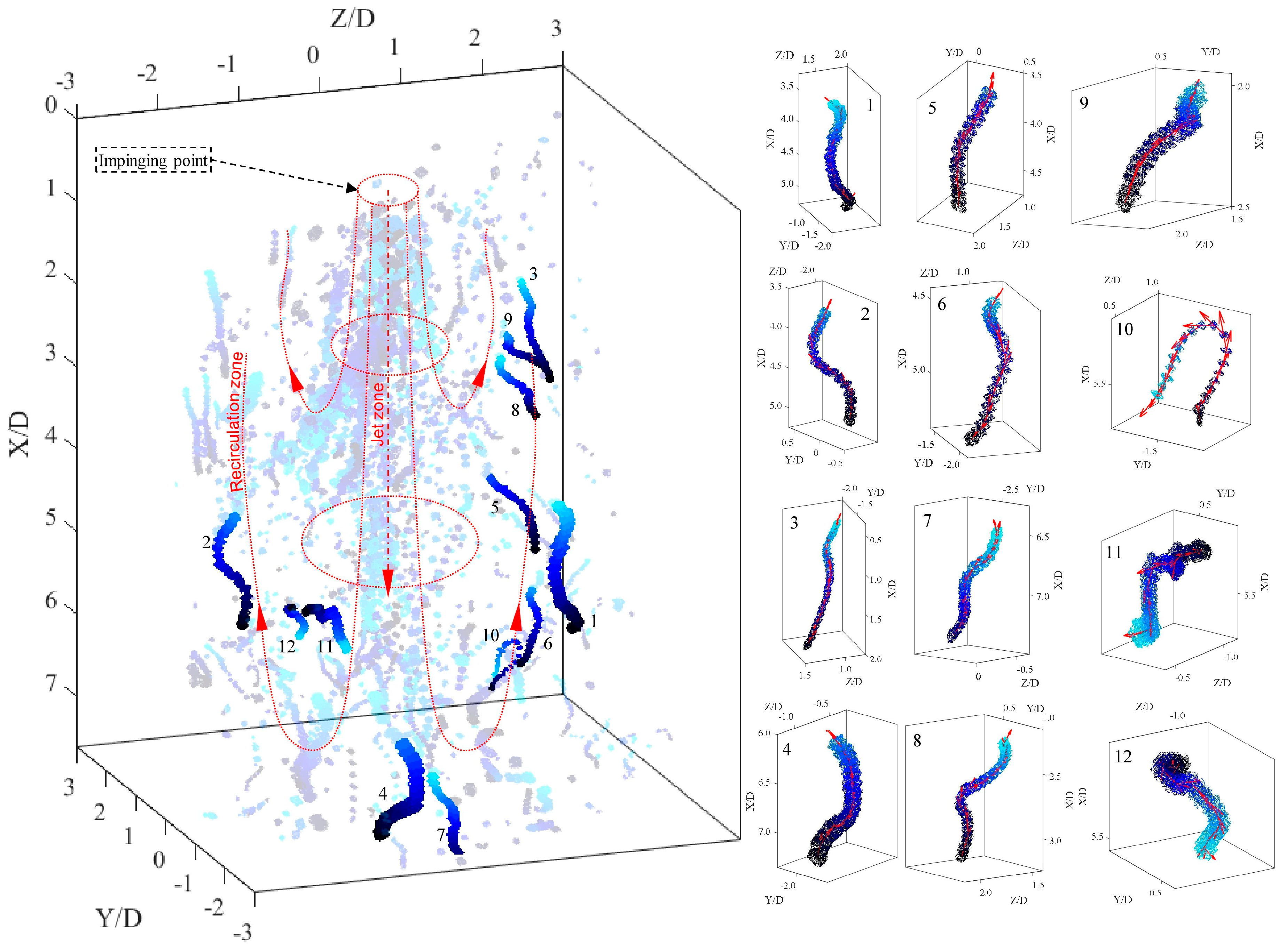
Figure 5 shows the reconstructed sequence of positions taken by selected air bubbles, composed of 26 consecutive frames. Some air bubbles have been observed inside the jet zone and show a vertical downwards path, some other bubbles move in the lateral recirculation zones with an upwards spiraling path.

2.3. Algorithms

2.3.1. Additive Regression of Decision Stumps

An additive regression model [52] aims to obtain forecasts by summing up the outcomes from other models: the weak learners. The procedure begins with the development of a standard regression model (e.g., a regression tree model). The errors in the training data, i.e., the differences between the algorithm predictions in the training values and the actual values are called residuals.
In order to correct these errors, another prediction model is built, generally of the same type as the former one, which tries to forecast the abovementioned residuals. For this purpose, the initial dataset is replaced by the attained residuals before training the second model. Adding the predictions of the second model to the forecasts of the first one allows us to reduce the amount of residuals. However, they are, again, different from zero because the second model is still not accurate enough. Thus, a third model is developed to predict the residuals of the residuals and the procedure is iterated, until a stopping rule based on cross-validation is met. In particular, a cross-validation is executed at each iteration up to a user-defined maximum number. The result that minimizes the cross-validation estimation of the squared error is selected. In this work, the algorithm performed 100 iterations for each of the considered models.
The Decision Stump algorithm has been chosen as weak learner. This algorithm is based on a one-level decision tree: one root node is directly linked to the terminal leaf nodes. A decision stump allows us to get a prediction on the base of the value of a single input feature: a threshold value is selected, and the stump is characterized by two leaves, respectively, for values above and below the threshold. There are also cases where multiple thresholds should be selected and the stump includes multiple leaves.

2.3.2. K-Star

The K-Star procedure [53] is an instance-based algorithm very similar to the k-Nearest Neighbor regression algorithm. The latter procedure provides a prediction by evaluating a weighted average of the k-nearest neighbors’ values, weighted by the inverse of their distance, and the Euclidean metric is typically used as distance metric. The innovative aspect of the K-Star algorithm is provided by the use of an entropy metric instead of Euclidean distance. The complexity of transforming one instance into another is chosen as the distance between the different instances. Complexity is evaluated by introducing a finite set of transformations among the instances and by defining the K* distance:
K * ( b | a ) = log 2 P r * ( b | a )
in which Pr* is the probability of all paths between instances a and b. If the instances are real numbers, it can be demonstrated that Pr*(b|a) is only dependent on the absolute value of the difference between a and b:
K * ( b | a ) = K * ( i ) = 1 2 log 2 ( 2 s s 2 ) log 2 ( s ) + i [ log 2 ( 1 s ) log 2 ( 1 2 s s 2 ) ]
In which i = |ab| and s is a parameter whose value is between zero and one. Consequently, the distance is a function of the absolute value of the difference between two instances. In addition, it can be assumed by the hypothesis that the real space is underlain by a discrete space, with the distance between the discrete instances being very small. In Equation (7), as s approaches zero, this leads to a probability density function, where the probability to obtain an integer between i and i + Δi is:
P r * ( i ) = s / 2 e i 2 s Δ i
which needs to be rescaled in terms of a real value x, where x / x o = i 2 s , in order to get the PDF of the real numbers:
P r * ( x ) = 1 2 x o e x x o d x
In practical uses, a realistic value of xo must be chosen, which is the mean expected value for x over the probability distribution. In the K-Star procedure, xo is chosen by selecting a number between no and N, where N is the whole number of training elements, while no is the number of the training elements at the smallest distance from a. The choice of xo is generally made by introducing the “blending parameter” b, which takes the value b = 0%, for no and b = 100%, for N, while intermediate values are linearly interpolated. For a more detailed description of the algorithm, see Cleary and Trigg [53]. A value of b = 40% has proven to be optimal for the problems addressed in this study.

2.3.3. Bagging and Random Forest

A regression tree essentially consists of a decision tree used as a predictive model [54]. Each internal node represents an input variable, while leaves correspond to specified real values of the target variables. The development of a regression tree consists of a recursive procedure in which the input data domain is divided into subdomains, while a multivariable linear regression model is employed to obtain predictions in each subdomain.
The recursive tree growth process is carried out by splitting each subdivision into smaller branches, considering all the possible splits in every field and detecting, at each step, the subdivision in two separate subsets minimizing the least squared deviation, defined as:
R ( t ) = 1 N ( t ) i t ( y i y m ( t ) ) 2
where N(t) is the number of sample elements in the t node, yi is the value of the target variable in the i-th element and ym is the average value of the target variable in the t node. This sum estimates the “impurity” at each node. The algorithm stops when the lowest impurity level is reached or if a different stopping rule is encountered.
The grouping of multiple learning models leads to an ensemble method, which may increase the forecast accuracy. The outcomes of different regression trees can be combined to get a single numeric result, for example, through a weighted average. Bootstrap aggregating, also known as Bagging, a ML algorithm introduced by Breiman, is based on such an approach: numerous training datasets of the same size are randomly picked, without replacement, from the original dataset in order to build a regression tree for each dataset. Different predictions will be provided by different regression trees, since small variations in the training dataset may lead to significant changes in ramifications and in outcomes for test instances. Bagging attempts to counteract the instability of the regression tree development process by varying the original training dataset instead of sampling a new independent training set each time: some instances are replaced by others. Finally, the individual predictions of the different regression trees are averaged.
The Random Forests algorithm is similar to the Bagging algorithm, but the procedure by which regression trees are built is different. Each node is allocated without considering the best subdivision among all the input variables, but by randomly choosing only a part of the variables to split on. The number of these variables does not change during the training process. Each tree is developed as far as possible, without pruning, until the minimum number of instances in a leaf node is reached.
In this study, the minimum number of leaf elements has been chosen to be equal to five, while each forest consists of 1000 trees.

2.3.4. Support Vector Regression

Starting from a training dataset {(x1, y1), (x2, y2), …, (xl, yl)} ⊂ X × R, where X is the space of the input arrays (e.g., XRn). Support Vector Regression (SVR) is a supervised learning algorithm [55] whose purpose is to find a function f(x) as flat as possible and with a maximum ε deviation from the observed target values yi. Therefore, given a linear function in the form:
f ( x ) = w , x + b
in which wX and bR, the Euclidean norm ||w||2 must be minimized, and this leads to a constrained convex optimization problem. In most cases, a significant error must be tolerated, so it is necessary to introduce slack variables ξι, ξι in the constraints. Consequently, the optimization problem can be formulated as follows:
minimize   1 2 w 2 + C i = 1 l ( ξ i + ξ i * )
subject   to   y i w , x i b ε + ξ i w , x i + b y i ε + ξ i *
where the function flatness and the tolerated deviations are dependent on the constant C > 0.
The SVR algorithm becomes nonlinear by pre-processing the training instances xi by means of a function Φ: XF, where F is some feature space. Since SVR only depends on the dot products between the different instances, a kernel k ( x i , x j ) = Φ ( x i ) , Φ ( x j ) can be used rather than explicitly using the function Φ(∙).
In this research, the Pearson VII universal function kernel (PUFK) has been selected:
k ( x i , x j ) = 1 [ 1 + ( ( 2 | x i x j | 2 2 ( 1 / ω ) 1 ) / σ ) 2 ] ω
in which the parameters σ and ω control the half-width and the tailing factor of the peak. In this study, the best results have been obtained for σ = 0.4 and ω = 0.4.

2.4. Evaluation Metrics and Cross-Validation

Different evaluation metrics have been used to assess the effectiveness of the predicting models: the coefficient of determination R2, the Mean Absolute Error (MAE), the Root Mean Squared Error (RMSE) and the Relative Absolute Error (RAE). These well-known metrics are defined below:
R 2 = ( 1 i = 1 m ( f i y i ) 2 i = 1 m ( y a y i ) 2 )
where m is the total number of experimental data, fi is the predicted value for data point i, and yi is the experimental value for data point i:
M A E = i = 1 m | f i y i | m
R M S E = i = 1 m ( f i y i ) 2 m
R A E = i = 1 m | f i y i | i = 1 m | y a y i |
in which ya is the averaged value of the observed data.
Each model has been built by a k-fold cross-validation process, using a set of about 300 vectors. The k-fold cross-validation involves the random subdivision of the original dataset into k subsets. Subsequently, k − 1 subsets are used to train the model, while the k-th single subset is reserved for testing and validating the model. The recurrent cross-validation procedure is carried out k times: each of the k subsets is used once as the testing dataset. Finally, the k results are averaged to obtain a single prediction. In this study, k = 10 has been assumed.

3. Results and Discussion

Different models were built to predict the equivalent diameter Deq after one time step, Deq+1, after two time steps, Deq+2 and, after three time steps, Deq+3. In the same way, different models were developed to forecast the aspect ratio AR after one time step, AR+1, after two time steps, AR+2 and, after three time steps, AR+3.
Based on the input variables, three different models were built for the prediction of Deq and AR. First, a model taking into account a greater number of variables that can affect the investigated phenomena was developed, then two simpler models were built, based on some relevant parameters for the evolution of the bubbles. Therefore, Model 1 is characterized by the following quantities as input variables: bubble velocity Vb, bubble depth below the free surface hb, the bubble Weber number Web, the bubble Froude number Frb, the bubble Reynolds number Reb, the Eötvös number Eo, the initial equivalent diameter Deq0. Model 2 admits as input variables Web, Reb and Eo. Model 3 has the following input variables: Web, Reb and Frb. In addition, five variants of each model were developed, changing the implemented machine learning algorithm.
Table 1 shows a comparison of the results provided by the different models. With regard to Deq+1, all models showed good predictive capabilities. Model 1 showed the best forecast performance, in all its variants. The Bagging algorithm proved to be the most accurate one in this case (R2 = 0.9749, MAE = 0.0974 mm, RMSE = 0.1434 mm, RAE = 13.42%), while the SVR-based variant led to less accurate predictions (R2 = 0.9472, MAE = 0.1418 mm, RMSE = 0.2020 mm, RAE = 20.18%). RF and K-Star showed a comparable performance, outperforming ARDS.
Model 2 exhibited forecasting capabilities very similar to those of Model 1. Furthermore, in this case, the Bagging algorithm (R2 = 0.9742, MAE = 0.0973 mm, RMSE = 0.1448 mm, RAE = 13.61%) led to the best predictions, while SVR (R2 = 0.9495, MAE = 0.1466 mm, RMSE = 0.2001 mm, RAE = 20.36%) was outperformed by all the other considered ones. RF showed an accuracy very close to that of Bagging, while the ARDS-based variant of Model 2 slightly outperformed the homologous variant of Model 1.
Model 3 was generally characterized by a significant decline in forecasting capabilities, however overall performance was still good. Unlike previous models, the SVR-based variant (R2 = 0.9546, MAE = 0.1388 mm, RMSE = 0.1931 mm, RAE = 19.10%) outperformed all the others. ARDS led to significantly less accurate predictions (R2 = 0.8425, MAE = 0.2710 mm, RMSE = 0.3552 mm, RAE = 36.80%), while RF ensured predictions comparable to those of SVR, outperforming both Bagging and K-Star.
As for Deq+2, Model 1 led to slightly less accurate results than those relating to the prediction of Deq+1. Again, the Bagging-based variant of Model 1 (R2 = 0.9650, MAE = 0.1284 mm, RMSE = 0.1675 mm, RAE = 17.35%) led to the most accurate predictions. On the other hand, SVR was, again, the worst performing algorithm (R2 = 0.9413, MAE = 0.1563 mm, RMSE = 0.2123 mm, RAE = 22.12%). RF and K-Star showed a comparable performance and both slightly outperformed ARDS.
Again, Model 2 predictive capabilities were just below those of Model 1 and Bagging algorithm led to the most accurate forecasts (R2 = 0.9590, MAE = 0.1403 mm, RMSE = 0.1820 mm, RAE = 18.88%), whereas SVR (R2 = 0.9434, MAE = 0.1655 mm, RMSE = 0.2144 mm, RAE = 22.39%) provided the least accurate outcomes. RF, ARDS and K-Star were characterized by their comparable forecasting capabilities in this case.
Model 3 was again characterized by a remarkable decrease in accuracy of forecasts, compared to Model 1 and Model 2, with a manifest increase in errors. As in the case of Deq+1, the SVR-based variant (R2 = 0.9410, MAE = 0.1619 mm, RMSE = 0.2147 mm, RAE = 22.58%) led to the best results, while the Bagging based variant (R2 = 0.9168, MAE = 0.1894 mm, RMSE = 0.2610 mm, RAE = 26.04%) provided the worst performance. RF outperformed both ARDS and Bagging. Moreover, the ARDS-based variant outperformed the homologous variant developed to forecast Deq+1.
Regarding Deq+3, the forecasting capabilities of Model 1 were in line with those of the homologous forecasting model of Deq+2. In this case RF led to the best forecasts (R2 = 0.9713, MAE = 0.1137 mm, RMSE = 0.1541 mm, RAE = 15.38%), while ARDS and SVR provided the least accurate results. Once again, the predictions of Model 2 were slightly less accurate than those of Model 1. The variant based on the Bagging algorithm (R2 = 0.670, MAE = 0.1204 mm, RMSE = 0.1670 mm, RAE = 16.17%) proved to be the best performing, while those based on ARDS and SVR also in this case led to the least accurate results. Model 3 confirmed itself as the worst performing model. Among the various variants of Model 3, the one based on SVR (R2 = 0.9416, MAE = 0.1590 mm, RMSE = 0.2162 mm, RAE = 21.74%) confirmed to be the most accurate, significantly outperforming all the others.
A comparative analysis of the three considered models, in all variants, showed that they do not undergo a significant reduction in forecasting capability of the equivalent diameter of the bubble, gradually passing from Deq+1 to Deq+2 and Deq+3. Therefore, with a good experimental dataset available, an approach based on machine learning may allow us to predict, with good accuracy, the variation in the bubble volume over time. Model 1 generally leads to the best predictions, but it requires a greater number of input variables and, in particular, it needs to know the initial depth of the bubble. Therefore, for practical purposes it may be better to use Model 2, whose high forecasting capabilities demonstrate that, to predict the volumetric deformation of the bubble with satisfactory accuracy, it is enough to know the initial values of the Weber, Reynolds and Eötvös numbers.
While it was established that, within Model 1 and Model 2, all the considered algorithms are able to provide good predictions, the variants based on the Bagging algorithm led to the best results, while those based on SVR provided the least accurate results. The latter algorithm, on the other hand, is the one that provided the best results within Model 3. However, Model 3 proved to be less accurate than the other two models: the absence of the number of Eötvös among the input variables significantly reduced its effectiveness. Moreover, it should be noted that the SVR algorithm has consistently shown the same level of accuracy across all models and input variables. This result highlights its robustness, as there is an indication that the algorithm is significantly sensitive to input parameters.
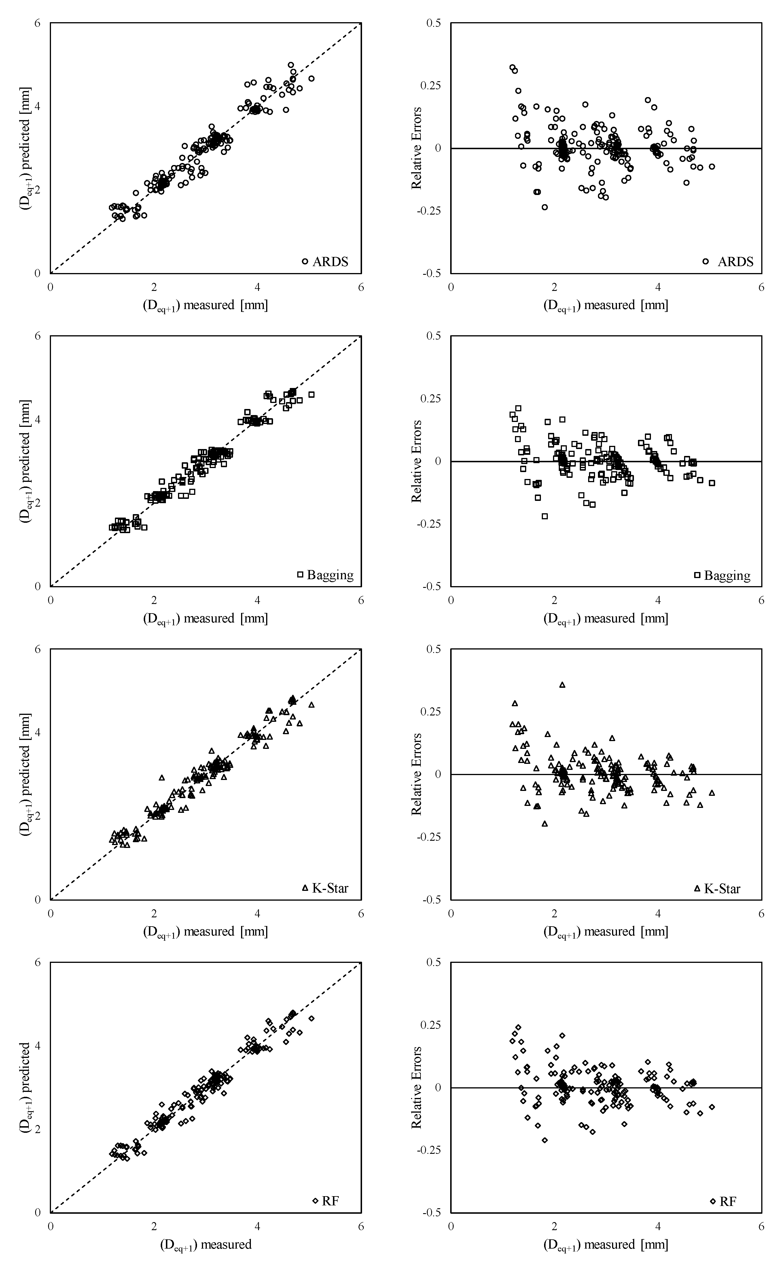
Figure 6 shows a comparison between the predicted and measured values of Deq+1, relative to Model 1. In addition, it shows the relative error as a function of the measured Deq+1. Overestimation errors were observed more frequently than underestimation errors in all Model 1 variants. Furthermore, the maximum relative errors were observed for bubbles with equivalent diameters less than 2 mm. These errors showed a tendency to decrease as the equivalent diameter grew and generally did not exceed ±25%. The exception was represented by the SVR algorithm. If the bubble diameter was less than 2 mm, SVR generally tended to overestimate the diameter itself and the error could also exceed 30%, while, if the diameter was greater than 4 mm, SVR tended to underestimate the diameter, with an error which did not exceed 15%. If the equivalent bubble diameter was between 2 and 4 mm, the SVR-based model variant provided results comparable to those of the other variants.
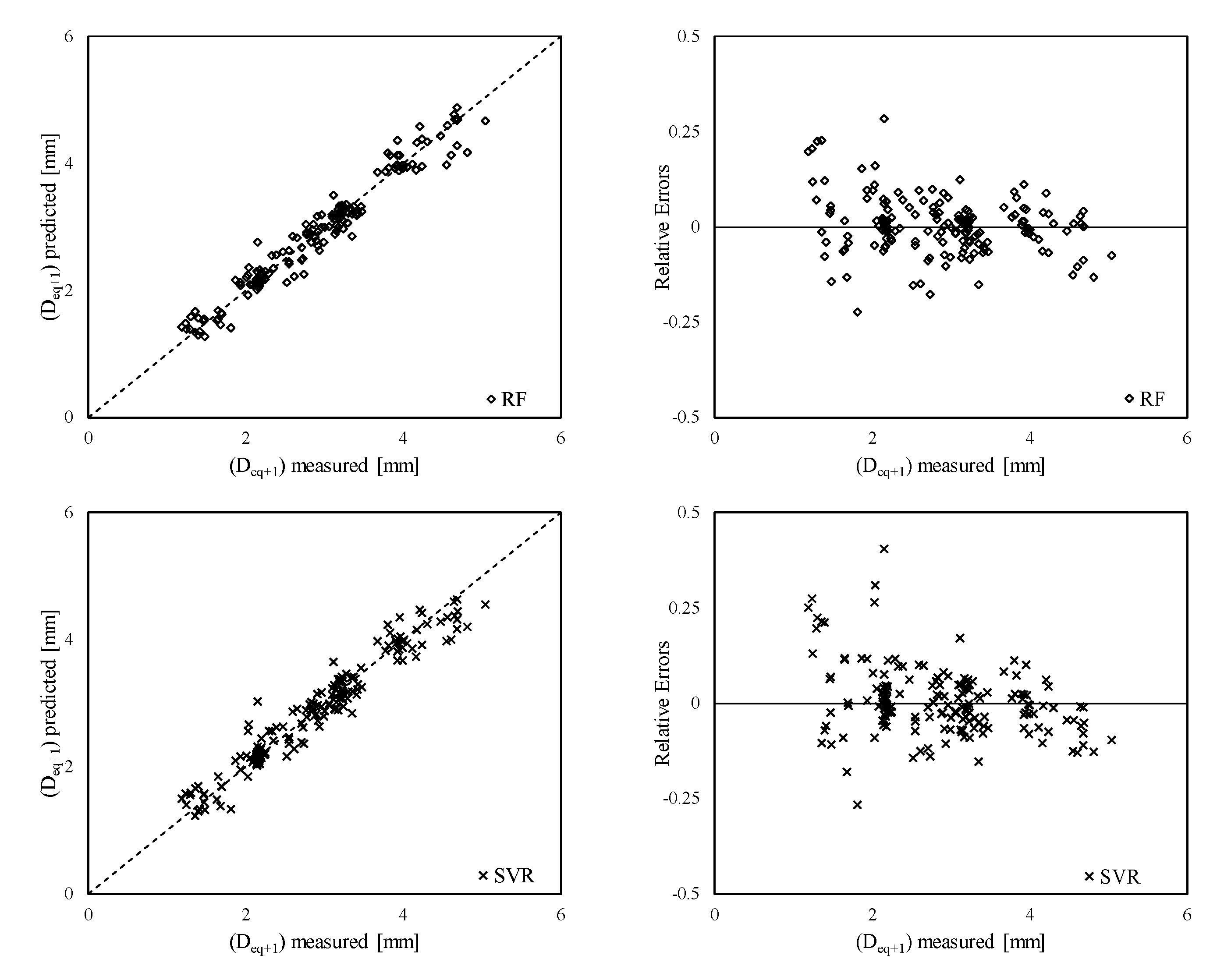
The comparison between the predicted and measured values of Deq+1 shown in Figure 7 relates to Model 2. As in the previous case, the same figure also shows the relative error as a function of the experimental Deq+1. The error distributions were quite similar to those of Model 1, while the maximum relative errors were observed when Deq < 2.5 mm. In this case, both K-Star and SVR led to relative errors, in some cases greater than 30% in the forecasts for smaller bubbles.
An alternative effective representation of the models’ errors in predicting Deq+1, in terms of residuals (i.e., absolute errors), is provided by the notched box plots in Figure 8. These plots show the range of errors with respect to the experimental values. The lower end of each box plot denotes the lower quartile Q1 (25th percentile), the upper end denotes the upper quartile Q3 (75th percentile), the band inside the box represents the median of the data. The whiskers extend from the bottom of the box to the smallest non-outlier and from the top of the box to the highest non-outlier in the dataset. The box plots further confirm what was previously argued in terms of the accuracy of the different models. It can also be noted that the variants of the models based on the Bagging and RF algorithms have their residual distributions characterized by greater symmetry than the others.
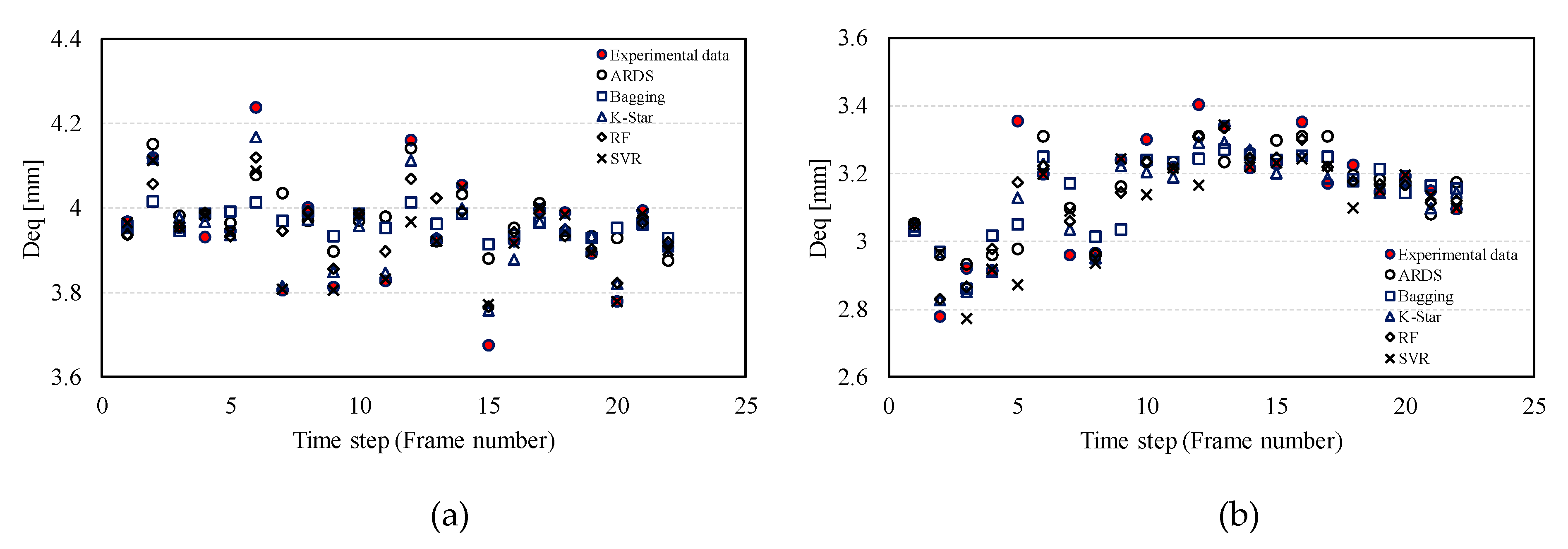
Figure 9 shows the Deq time series of two of the analyzed bubbles. Again, it can be observed that all models’ variants provided predictions in good agreement with the experimental data. In addition, it is interesting to note that higher errors were observed in correspondence with higher changes in the experimental values between two consecutive time steps. Finally, it may be worth highlighting that the algorithm that provided the most accurate predictions for a single bubble may be different from the algorithm that was the most accurate in the entire dataset.
The aspect ratio (AR) results are summarized in Table 2. The accuracy of the prediction models was significantly lower than that of the analogous forecast models of equivalent diameter.
With regard to AR+1, Model 1 showed again the best prediction capability and the ARDS algorithm was the most accurate one (R2 = 0.5376, MAE = 0.0244, RMSE = 0.0317, RAE = 67.89%), while all the other considered algorithms showed comparable performances. Model 2 showed an appreciable deterioration in forecasting capabilities compared to Model 1, except for the SVR-based variant. The results of Model 3 were even less accurate, especially those of the ARDS-based variant.
As for AR+2, Model 1 outcomes were comparable to the results of the homologous predictive model of AR+1, in some cases even slightly better. Model 2 predictions also had an accuracy similar to that of Model 1. In particular, from the comparison with Model 1, by analyzing the results of the different Model 2 variants, it could be observed that ARDS was characterized by the deterioration of the predictive capabilities, while K-Star showed an improvement. For the other algorithms, the different metrics led to conflicting results. Model 3 proved to be the less accurate once again, except for the SVR-based variant, which outperformed the analogous variant of Model 2. As for AR+3, Model 2 outperformed Model 1 in all variants, while Model 3 led to the least accurate predictions, except for the SVR-based variant, the results of which are comparable to the analogous variant of Model 2.
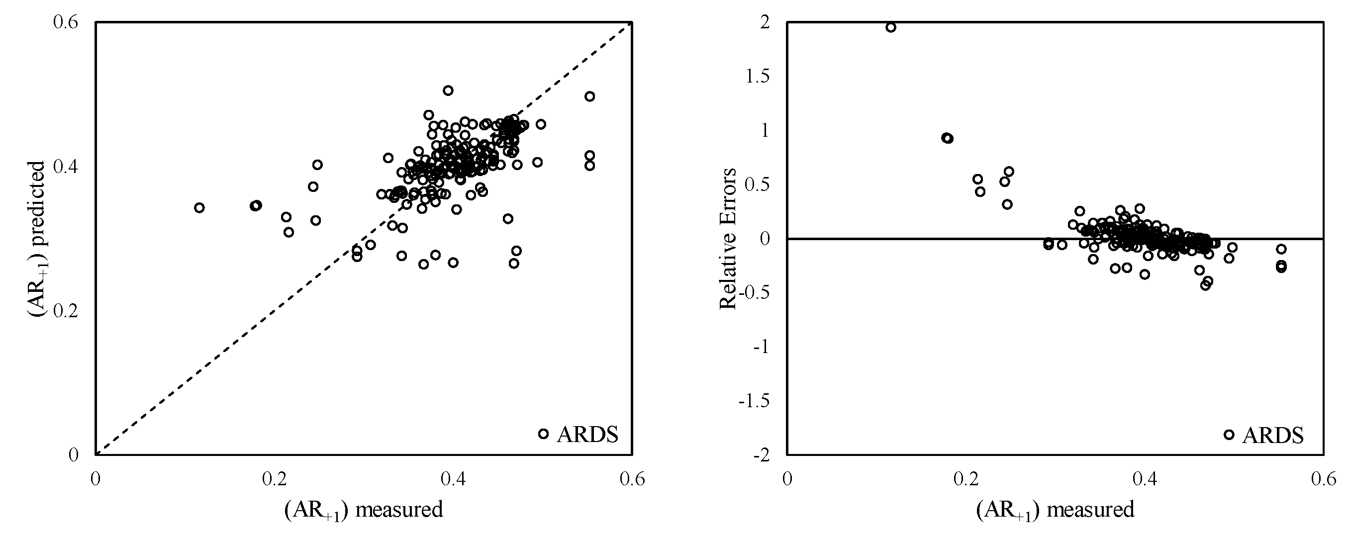
Figure 10 shows a comparison between the predicted and experimental values of AR+1, with reference to Model 1. In addition, it shows the relative error versus the measured AR+1.
It is evident that the results which most negatively affect the metrics refer to AR < 0.3. In this range, the model outcomes were particularly poor. This occurrence was mainly due to the scarcity of training data falling within this range. However, it should be noted that the models’ predictions cannot be considered satisfactory in the entire investigated experimental range. There was an important limitation in the model, which did not include, among the input variables, a parameter that adequately takes into account the stress state on the surface of the bubbles (i.e., pressure and shear stress in the liquid surrounding the bubble). Unfortunately, measurements carried out via shadowgraph technique are not able to overcome this limitation.
For the sake of brevity, the diagrams relating to the similar Model 2 results and the poorer Model 3 results are not shown.
Figure 11 shows the notched box plots of the residuals in AR+1 predictions. The box plots also show quite clearly that Model 1 outperforms Model 2, which, in turn, outperforms Model 3. Furthermore, the number of outliers is significant. Finally, the distributions of the residuals are slightly asymmetric, with a prevalence of positive values.
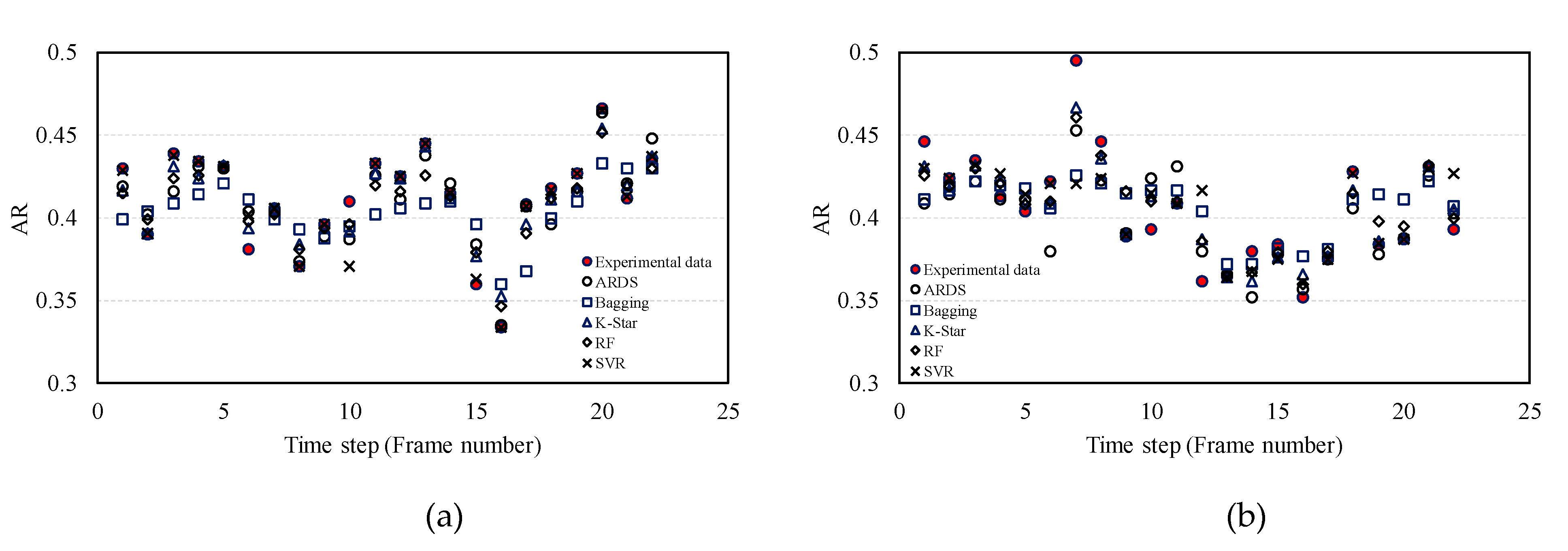
Figure 12 shows the AR time series of two of the analyzed bubbles. The results are better than what was expected on the basis of the analysis carried out above. They confirm that the model evaluation metrics have been significantly worsened by the results relating to bubbles characterized by very low aspect ratios. Therefore, it is reasonable to believe that the forecast models based on machine learning algorithms are able to provide accurate predictions of the aspect ratio of single bubbles, when used for bubbles whose characteristics are comparable to those used for model training.
Model 2, based on the numbers of Weber, Reynolds and Eötvös only, has proven to be able to predict, with good approximation, the evolution of single bubbles, in terms of equivalent diameter and aspect ratio, in a field of uncertain pressures originating from a plunging jet. The combination of Web, Frb and Reb leads to an additional dimensionless parameter, indicated as Morton number Mo:
M o = W e b 3 F r b 2 Re b 4
However, it is not useful to introduce a new parameter into prediction models that is a combination of already considered parameters, nor is it possible to define a simple functional relationship between the deformation of a single bubble and the Morton number. Therefore, this parameter has not been considered in this study.
Overall, preliminary elaborations have shown that, with regard to the equivalent diameter, the number of tracked bubbles is sufficient for the convergence of the model. If a single bubble is excluded from the training dataset, the developed models still lead to results quite close to those obtained from the entire dataset. Instead, regarding the aspect ratio, a greater number of bubbles in the AR < 0.3 range could improve the accuracy of the models.

4. Conclusions

A truthful prediction of the deformation of air bubbles in a water volume in the presence of uncertain pressure field is an important aspect of the study of phenomena such as cavitation, air entrainment and foaming. If suitable experimental data are available, machine learning algorithms can provide powerful tools to obtain accurate predictions.
In this study, three different models were built to predict the equivalent diameter and aspect ratio of air bubbles moving near a plunging jet. Five variants of each model were developed, varying the implemented machine learning algorithm: Additive Regression of Decision Stump, Bagging, K-Star, Random Forest and Support Vector Regression. The experimental data were obtained from measurements carried out using a shadowgraph technique.
As for the prediction of the equivalent diameter, Model 1 provided the best predictions in most cases, but it needs a higher number of input variables, including the initial depth of the bubble. Model 2 provided results comparable to those of Model 1, but requires only the Reynolds, Weber and Eötvös numbers as inputs. The lower accuracy of Model 3 can be attributed to the absence of the number of Eötvös among the input variables. Within Model 1 and Model 2, the variant based on the Bagging algorithm led to the best results in most cases, while the variant based on SVR led to the least accurate results. On the other hand, the SVR-based variant provided the best results under Model 3.
Regarding the forecast of the aspect ratio, the results of the three models cannot be considered fully satisfactory in general, even if, for some bubbles, the models have provided very good predictions. The unsatisfactory results can be attributed to the training dataset, which does not include an adequate number of bubbles with low aspect ratio values, and probably to the limits of the models, whose input variables do not adequately take into account the stresses acting on the surface of the bubbles.
From what is shown in this study, it is therefore clear that a combined approach based on a shadowgraph technique and machine learning algorithms can certainly be considered to address complex problems in the study of multi-phase flows.

Author Contributions

Conceptualization, F.G.; methodology, F.G. and F.D.N.; software, F.G.; validation, F.D.N, F.A.P, F.D.F, G.d.M., R.G. and M.M.; formal analysis: F.G. and F.D.N.; investigation: F.G., F.D.N., F.A.P., F.D.F., G.d.M., R.G. and M.M.; data curation: F.D.N.; writing—original draft preparation, F.G. and F.D.N.; writing—review and editing: F.A.P., F.D.F., G.d.M., M.M. and R.G.; supervision: F.G. All authors have read and agreed to the published version of the manuscript.

Funding

The work described here was conducted as part of the Italian Ministry of Education, University and Research 2017 PRIN Project ACE, grant 2017RSH3JY.

Conflicts of Interest

The authors declare no conflict of interest.

References

  1. Rayleigh, L. On the pressure developed in a liquid during the collapse of a spherical cavity. Philos. Mag. 1919, 34, 94–98. [Google Scholar] [CrossRef]
  2. Plesset, M.S. The dynamics of cavitation bubbles. J. Appl. Mech. 1949, 16, 228–231. [Google Scholar] [CrossRef]
  3. Gilmore, F.R. The Growth or Collapse of a Spherical Bubble in a Viscous Compressible Liquid; California Institute of Technology: Pasadena, CA, USA, 1952; Unpublished. [Google Scholar]
  4. Fujikawa, S.; Akamatsu, T. Effects of the non-equilibrium condensation of vapour on the pressure wave produced by the collapse of a bubble in a liquid. J. Fluid Mech. 1980, 97, 3–512. [Google Scholar] [CrossRef]
  5. Keller, J.B.; Miksis, M. Bubble oscillations of large amplitude. J. Acoust. Soc. Am. 1980, 68, 2–633. [Google Scholar] [CrossRef] [Green Version]
  6. Prosperetti, A.; Crum, L.A.; Commander, K.W. Nonlinear bubble dynamics. J. Acoust. Soc. Am. 1988, 83, 2–514. [Google Scholar] [CrossRef]
  7. Fujiwara, A.; Danmoto, Y.; Hishida, K.; Maeda, M. Bubble deformation and flow structure measured by double shadow images and PIV/LIF. Exp. Fluids 2004, 36, 1–165. [Google Scholar] [CrossRef]
  8. Cao, Y.; Kawara, Z.; Yokomine, T.; Kunugi, T. Experimental and numerical study on nucleate bubble deformation in subcooled flow boiling. Int. J. Multiph. Flow 2016, 82, 93–105. [Google Scholar] [CrossRef]
  9. Feng, J.; Cao, J.; Jiang, J.; Sun, B.; Cai, Z.; Gao, Z. Single bubble breakup in the flow field induced by a horizontal jet—The experimental research. Asia Pac. J. Chem. Eng. 2019, 14, 1. [Google Scholar] [CrossRef] [Green Version]
  10. Korobeynikov, S.M.; Ridel, A.V.; Medvedev, D.A. Deformation of bubbles in transformer oil at the action of alternating electric field. Eur. J. Mech. B Fluids 2019, 75, 105–109. [Google Scholar] [CrossRef]
  11. Ekambara, K.; Dhotre, M.T.; Joshi, J.B. CFD simulations of bubble column reactors: 1D, 2D and 3D approach. Chem. Eng. Sci. 2005, 60, 23–6746. [Google Scholar] [CrossRef]
  12. Kerdouss, F.; Bannari, A.; Proulx, P. CFD modeling of gas dispersion and bubble size in a double turbine stirred tank. Chem. Eng. Sci. 2006, 61, 10–3322. [Google Scholar] [CrossRef]
  13. Rzehak, R.; Krepper, E. CFD modeling of bubble-induced turbulence. Int. J. Multiph. Flow 2013, 55, 138–155. [Google Scholar] [CrossRef]
  14. Fletcher, D.F.; McClure, D.D.; Kavanagh, J.M.; Barton, G.W. CFD simulation of industrial bubble columns: Numerical challenges and model validation successes. Appl. Math. Model. 2017, 44, 25–42. [Google Scholar] [CrossRef]
  15. Pfister, M.; Chanson, H. Two-phase air-water flows: Scale effects in physical modeling. J. Hydrodyn. Ser. B 2014, 26, 2–298. [Google Scholar] [CrossRef] [Green Version]
  16. Schmidt, E. Ähnlichkeitstheorie der Bewegung von Flüssigkeitsgasgemsichen (Similarity Theory of Motion in Fluid-Gas Mixtures). Forschungsheft 1934, 365, 1–3. (In German) [Google Scholar]
  17. Clift, R.; Grace, J.; Weber, M. Bubbles, Drops, and Particles; Academic Press: New York, NY, USA, 1978; p. 380. [Google Scholar]
  18. Tripathi, M.; Sahu, K.; Govindarajan, R. Dynamics of an initially spherical bubble rising in quiescent liquid. Nat. Commun. 2015, 6, 6268. [Google Scholar] [CrossRef] [Green Version]
  19. Cummings, P.D.; Chanson, H. Air Entrainment in the Developing Flow Region of Plunging Jets—Part 1: Theoretical Development. J. Fluids Eng. Trans. ASME 1997, 119, 3–602. [Google Scholar] [CrossRef] [Green Version]
  20. Ervine, D.A.; Falvey, H.T.; Withers, W.A. Pressure fluctuations on plunge pool floors. J. Hydraul. Res. 1997, 35, 257–279. [Google Scholar] [CrossRef]
  21. Liao, Y.; Rzehak, R.; Lucas, D.; Krepper, E. Baseline closure model for dispersed bubbly flow: Bubble coalescence and breakup. Chem. Eng. Sci. 2015, 122, 336–349. [Google Scholar] [CrossRef]
  22. Lunde, K.; Perkins, R.J. Shape Oscillations of Rising Bubbles. Flow Turbul. Combust. 1997, 58, 387–408. [Google Scholar]
  23. Avdeev, A.A. Bubble Systems; Springer International Publishing: Berlin/Heidelberg, Germany, 2016. [Google Scholar]
  24. Solomatine, D.P.; Xue, Y. M5 Model Trees and Neural Networks: Application to Flood Forecasting in the Upper Reach of the Huai River in China. J. Hydrol. Eng. 2004, 9, 6–501. [Google Scholar] [CrossRef]
  25. Ahmad, S.; Kalra, A.; Stephen, H. Estimating soil moisture using remote sensing data: A machine learning approach. Adv. Water Resour. 2010, 33, 1–80. [Google Scholar] [CrossRef]
  26. Nourani, V.; Kisi, Ö.; Komasi, M. Two hybrid artificial intelligence approaches for modeling rainfall–runoff process. J. Hydrol. 2011, 402, 41–59. [Google Scholar] [CrossRef]
  27. Kisi, O. Modeling discharge-suspended sediment relationship using least square support vector machine. J. Hydrol. 2012, 456, 110–120. [Google Scholar] [CrossRef]
  28. Najafzadeh, M.; Etemad-Shahidi, A.; Lim, S.Y. Scour prediction in long contractions using ANFIS and SVM. Ocean Eng. 2016, 111, 128–135. [Google Scholar] [CrossRef]
  29. Granata, F.; Papirio, S.; Esposito, G.; Gargano, R.; De Marinis, G. Machine learning algorithms for the forecasting of wastewater quality indicators. Water 2017, 9, 2. [Google Scholar] [CrossRef] [Green Version]
  30. Naghibi, S.A.; Ahmadi, K.; Daneshi, A. Application of support vector machine, random forest, and genetic algorithm optimized random forest models in groundwater potential mapping. Water Resour. Manag. 2017, 31, 9–2775. [Google Scholar] [CrossRef]
  31. Granata, F. Evapotranspiration evaluation models based on machine learning algorithms—A comparative study. Agric. Water Manag. 2019, 217, 303–315. [Google Scholar] [CrossRef]
  32. Arnon, T.A.; Ezra, S.; Fishbain, B. Water characterization and early contamination detection in highly varying stochastic background water, based on Machine Learning methodology for processing real- time UV-Spectrophotometry. Water Res. 2019, 155, 333–342. [Google Scholar] [CrossRef]
  33. Granata, F.; Di Nunno, F.; Gargano, R.; de Marinis, G. Equivalent Discharge Coefficient of Side Weirs in Circular Channel—A Lazy Machine Learning Approach. Water 2019, 11, 11. [Google Scholar] [CrossRef] [Green Version]
  34. Granata, F.; Gargano, R.; de Marinis, G. Artificial intelligence based approaches to evaluate actual evapotranspiration in wetlands. Sci. Total Environ. 2020, 703, 135653. [Google Scholar] [CrossRef] [PubMed]
  35. Shaban, H.; Tavoularis, S. Measurement of gas and liquid flow rates in two-phase pipe flows by the application of machine learning techniques to differential pressure signals. Int. J. Multiph. Flow 2014, 67, 106–117. [Google Scholar] [CrossRef]
  36. Granata, F.; de Marinis, G. Machine learning methods for wastewater hydraulics. Flow Meas. Instrum. 2017, 57, 1–9. [Google Scholar] [CrossRef]
  37. Mosavi, A.; Shamshirband, S.; Salwana, E.; Chau, K.W.; Tah, J.H. Prediction of multi-inputs bubble column reactor using a novel hybrid model of computational fluid dynamics and machine learning. Eng. Appl. Comput. Fluid Mech. 2019, 13, 1–492. [Google Scholar] [CrossRef]
  38. Li, Q.; Griffiths, J.G. Least squares ellipsoid specific fitting. In Proceedings of the Geometric Modeling and Processing, Beijing, China, 13–15 April 2004; pp. 335–340. [Google Scholar]
  39. Pereira, F.; Avellan, F.; Dupont, P. Prediction of cavitation erosion: An energy approach. J. Fluids Eng. 1998, 120, 4–727. [Google Scholar] [CrossRef]
  40. Di Nunno, F.; Alves Pereira, F.; Granata, F.; de Marinis, G.; Di Felice, F.; Gargano, R.; Miozzi, M. A shadowgraphy approach for the 3D Lagrangian description of bubbly flows. Meas. Sci. Technol. 2020, in press. [Google Scholar] [CrossRef]
  41. Tsai, R.Y. An Efficient and Accurate Camera Calibration Technique for 3D Machine Vision. In Proceedings of the Computer Vision and Pattern Recognition, Miami Beach, FL, USA, 22–26 June 1986; pp. 364–374. [Google Scholar]
  42. Trucco, E.; Verri, A. Introductory Techniques for 3-D Computer Vision; Prentice Hall: Englewood Cliffs, NJ, USA, 1998; p. 343. [Google Scholar]
  43. Zhang, Z. A flexible new technique for camera calibration. IEEE Trans. Pattern Anal. Mach. Intell. 2000, 22, 1330–1334. [Google Scholar] [CrossRef] [Green Version]
  44. Fu, Y.; Liu, Y. 3D bubble reconstruction using multiple cameras and space carving method. Meas. Sci. Technol. 2018, 29, 7. [Google Scholar] [CrossRef]
  45. Ridler, T.; Calvard, S. Picture thresholding using an iterative selection method. IEEE Trans. Syst. Man Cybern. SMC-8 1978, 8, 630–632. [Google Scholar]
  46. Vincent, L.; Soille, P. Watersheds in digital spaces: An efficient algorithm based on immersion simulations. IEEE Trans. Pattern Anal. Mach. Intell. 1991, 13, 6–598. [Google Scholar] [CrossRef] [Green Version]
  47. Di Nunno, F.; Alves Pereira, F.; de Marinis, G.; Di Felice, F.; Gargano, R.; Granata, F.; Miozzi, M. Experimental study of air-water two-phase jet: Bubble size distribution and velocity measurements. J. Phys. Conf. Ser. 2018, 1110, 012011. [Google Scholar]
  48. Di Nunno, F.; Alves Pereira, F.; de Marinis, G.; Di Felice, F.; Gargano, R.; Granata, F.; Miozzi, M. Two-phase PIV-LIF measurements in a submerged bubbly water jet. J. Hydraul. Eng. 2019, 145, 9. [Google Scholar] [CrossRef]
  49. Lucas, B.; Kanade, T. An Iterative Image Registration Technique with an Application to Stereo Vision. In Proceedings of the 7th International Joint Conference on Artificial Intelligence, Vancouver, BC, Canada, 24–28 August 1981; pp. 121–130. [Google Scholar]
  50. Miozzi, M.; Jacob, B.; Olivieri, A. Performances of feature tracking in turbulent boundary layer investigation. Exp. Fluids 2008, 45, 4–780. [Google Scholar] [CrossRef]
  51. Fdida, N.; Blaisot, J.B. Drop size distribution measured by imaging: Determination of the measurement volume by the calibration of the point spread function. Meas. Sci. Technol. 2009, 21, 2. [Google Scholar] [CrossRef]
  52. Witten, I.H.; Frank, E.; Hall, M.A.; Pal, C.J. Data Mining: Practical Machine Learning Tools and Techniques, 2nd ed.; Morgan Kaufmann: Burlington, VT, USA, 2016; p. 560. [Google Scholar]
  53. Cleary, J.G.; Trigg, L.E. K*: An instance based learner using an entropic distance measure. In Proceedings of the 12th International Conference on Machine Learning, Tahoe City, CA, USA, 9–12 July 1995; pp. 108–114. [Google Scholar]
  54. Breiman, L.; Friedman, J.; Stone, C.J.; Olshen, R.A. Classification and Regression Trees; Taylor & Francis: Abingdon, UK, 1984; p. 368. [Google Scholar]
  55. Cortes, C.; Vapnik, V. Support-vector networks. Mach. Learn. 1995, 20, 273–297. [Google Scholar] [CrossRef]
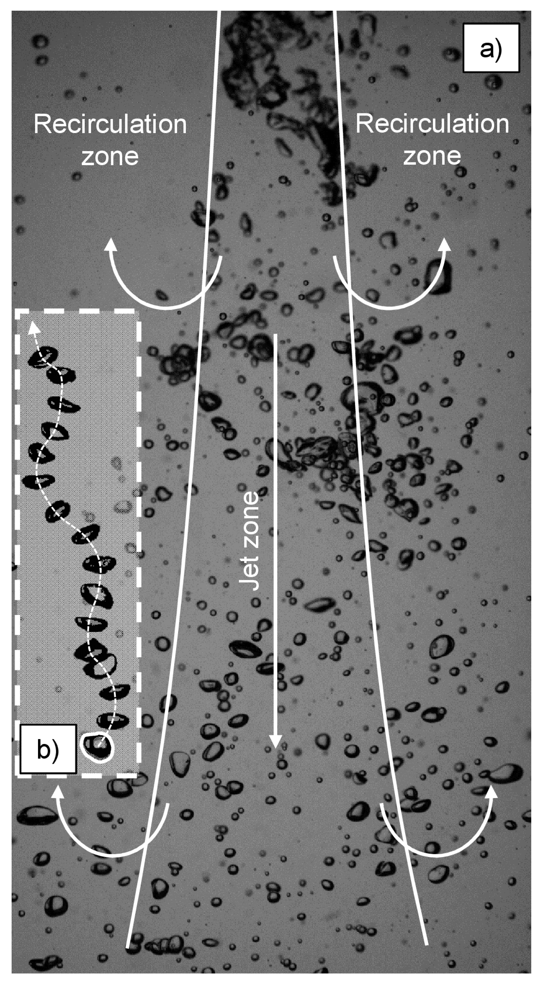
Figure 1. Air bubbles entrained by the vertical plunging jet (a); individual air bubble path, rising inside the lateral recirculation zone (only the highlighted bubble is at the same time as the recorded frame) (b).
Applsci 10 03879 g001
Figure 2. Experimental setup.
Applsci 10 03879 g002
Figure 3. Measurement principle.
Applsci 10 03879 g003
Figure 4. Steps for the boundary detection: original image (a); image after background removal (b); binary image (c); image after watershed operation (d); final image containing the outline of the detected air bubbles (e).
Applsci 10 03879 g004
Figure 5. Sequence of air bubbles entrained by the vertical plunging jet and reconstructed by means of the volumetric shadowgraph technique. The plunging jet is downward from the top, with X/D = 0 indicating the water surface.
Applsci 10 03879 g005
Figure 6. Equivalent diameter prediction “Model 1”: in the left column, predicted versus experimental values, in the right column, residuals versus experimental values.
Applsci 10 03879 g006aApplsci 10 03879 g006b
Figure 7. Equivalent diameter prediction “Model 2”: in the left column, predicted versus experimental values, in the right column, residuals versus experimental values.
Applsci 10 03879 g007aApplsci 10 03879 g007b
Figure 8. Equivalent diameter prediction: box plots of the residuals.
Applsci 10 03879 g008
Figure 9. Comparison among equivalent diameters by means of time series; (a) Model 1—bubble 1; (b) Model 2—bubble 12.
Applsci 10 03879 g009
Figure 10. Aspect ratio prediction “Model 1”: in the left column, predicted versus experimental values, in the right column, residuals versus experimental values.
Applsci 10 03879 g010aApplsci 10 03879 g010b
Figure 11. Aspect ratio prediction: box plots of the residuals.
Applsci 10 03879 g011
Figure 12. Comparison among aspect ratios by means of time series; (a) Model 1—bubble 1; (b) Model 2—bubble 12.
Applsci 10 03879 g012
Table 1. Synthesis of the results of equivalent diameter (Deq) prediction models.
Model NumberInput VariablesAlgorithmR2MAE [mm]RMSE [mm]RAE
Deq+11hb, Vb, Web, Frb, Reb, Eo, Deq0ARDS0.96710.11320.168615.39%
Bagging0.97490.09740.143413.42%
K-Star0.96920.11110.158215.27%
RF0.97340.10470.148914.33%
SVR0.94720.14180.202020.18%
2Web, Reb, EoARDS0.96400.12090.174816.31%
Bagging0.97420.09730.144813.61%
K-Star0.96290.11520.171716.29%
RF0.96760.11380.164515.42%
SVR0.94950.14660.200120.36%
3Web, Frb, RebARDS0.84250.27100.355236.80%
Bagging0.92690.17060.246123.38%
K-Star0.92140.17490.248824.68%
RF0.95120.13540.203218.52%
SVR0.95460.13880.193119.10%
Deq+21hb, Vb, Web, Frb, Reb, Eo, Deq0ARDS0.95360.14950.193620.04%
Bagging0.96500.12840.167517.35%
K-Star0.96510.12780.168717.38%
RF0.96370.13460.171518.15%
SVR0.94130.15630.212322.12%
2Web, Reb, EoARDS0.94990.15550.200920.77%
Bagging0.95900.14030.182018.88%
K-Star0.94810.14950.200320.86%
RF0.95530.15070.189820.32%
SVR0.94340.16550.214422.39%
3Web, Frb, RebARDS0.92610.18990.247025.75%
Bagging0.91680.18940.261026.04%
K-Star0.91700.18430.258025.77%
RF0.93860.16820.225422.85%
SVR0.94100.16190.214722.58%
Deq+31hb, Vb, Web, Frb, Reb, Eo, Deq0ARDS0.95260.14370.198019.29%
Bagging0.96950.11810.158915.84%
K-Star0.96390.12720.170517.28%
RF0.97130.11370.154115.38%
SVR0.93990.15550.215321.92%
2Web, Reb, EoARDS0.94510.15700.210721.10%
Bagging0.96700.12040.167016.17%
K-Star0.94220.14710.209420.86%
RF0.96320.12850.173417.39%
SVR0.94250.16450.213322.58%
3Web, Frb, RebARDS0.89320.21890.295029.47%
Bagging0.88450.22280.303630.51%
K-Star0.90310.19710.277227.79%
RF0.91700.19740.262326.45%
SVR0.94160.15900.216221.74%
Table 2. Synthesis of the results of aspect ratio (AR) prediction models.
Model NumberInput VariablesAlgorithmR2MAERMSERAE
AR+11hb, Vb, Web, Frb, Reb, Eo, Deq0ARDS0.53760.02440.031767.89%
Bagging0.46510.02540.034269.85%
K-Star0.35050.02770.037276.64%
RF0.40020.02760.038472.71%
SVR0.29760.02720.037376.96%
2Web, Reb, EoARDS0.47950.02830.037272.86%
Bagging0.38840.02860.037677.28%
K-Star0.35730.02770.036977.11%
RF0.33020.03030.040779.89%
SVR0.36370.02790.037476.38%
3Web, Frb, RebARDS0.14630.04000.0540107.30%
Bagging0.19570.03210.042985.76%
K-Star0.22570.03110.041783.70%
RF0.20380.03030.040684.40%
SVR0.30230.02870.038779.55%
AR+21hb, Vb, Web, Frb, Reb, Eo, Deq0ARDS0.46280.02840.038572.66%
Bagging0.34010.02940.038680.03%
K-Star0.37830.03080.042077.99%
RF0.37720.03000.040978.33%
SVR0.40350.02800.037175.81%
2Web, Reb, EoARDS0.33540.03320.043983.01%
Bagging0.36590.03120.040480.95%
K-Star0.44590.03150.041177.78%
RF0.44160.03110.041776.21%
SVR0.42420.03320.043280.22%
3Web, Frb, RebARDS0.05570.04340.0547105.91%
Bagging0.32820.03490.043486.55%
K-Star0.42260.03280.041180.80%
RF0.34660.03440.044884.39%
SVR0.45380.03340.042280.08%
AR+31hb, Vb, Web, Frb, Reb, Eo, Deq0ARDS0.13640.03580.046893.19%
Bagging0.33940.03010.039380.06%
K-Star0.16620.03450.045789.14%
RF0.30650.03150.041381.96%
SVR0.22930.03010.040383.25%
2Web, Reb, EoARDS0.43270.02950.038875.35%
Bagging0.38780.03020.038978.77%
K-Star0.32580.03140.039984.21%
RF0.31900.03150.041182.30%
SVR0.32320.02940.039679.09%
3Web, Frb, RebARDS0.03710.04060.0511104.77%
Bagging0.16540.03550.044992.77%
K-Star0.23690.03370.043088.32%
RF0.23540.03360.043088.87%
SVR0.35010.03220.041183.04%