A Long Short-Term Memory (LSTM) Network for Hourly Estimation of PM_2.5 Concentration in Two Cities of South Korea

Featured Application

Forecasting particulate matter of size less than 2.5 µm (PM${}_{2.5}$) in big cities is a major challenge for scientific community. In addition to environmental impacts, these particulate matter cause various diseases, such as cardiopulmonary disease, stroke, lung cancer and even neurological disorders. Forecasting high PM${}_{2.5}$ events helps to raise awareness among people to take precautionary measures, such as limit outdoor activities, use masks, etc. In the future, advanced Machine Learning (ML) based PM${}_{2.5}$ forecasting will help to reduce the cost of sampling of PM${}_{2.5}$, such as sampler and equipment costs, which are needed to measure the concentration of particulate matter in air.

Abstract

Air pollution not only damages the environment but also leads to various illnesses such as respiratory tract and cardiovascular diseases. Nowadays, estimating air pollutants concentration is becoming very important so that people can prepare themselves for the hazardous impact of air pollution beforehand. Various deterministic models have been used to forecast air pollution. In this study, along with various pollutants and meteorological parameters, we also use the concentration of the pollutants predicted by the community multiscale air quality (CMAQ) model which are strongly related to PM${}_{2.5}$ concentration. After combining these parameters, we implement various machine learning models to predict the hourly forecast of PM${}_{2.5}$ concentration in two big cities of South Korea and compare their results. It has been shown that Long Short Term Memory network outperforms other well-known gradient tree boosting models, recurrent, and convolutional neural networks.

1. Introduction

The industrial revolution and modernization have led us to a new era of science and technology. On the one hand, it has opened new horizons for transportation, trade, mining, agriculture, and urbanization. On the other hand, it has become a vital factor in polluting air, soil, and water. In the last two decades, many environmental researchers have been monitoring the quality of ambient air. Particulate matter (PM) is found to be the most dangerous kind of air pollution among various other air pollutants. After a study done by the World Health Organization (WHO) and the International Agency of Research center (IARC), PM in ambient air has been categorized as ‘carcinogenic’ [1,2]. PM${}_{2.5}$ are the fine particulate matters with size less than 2.5 micrometer which are the major cause of allergies, pulmonary, and cardiovascular diseases, morbidity, and mortality. Various epidemiological tests [3] have shown a direct relationship between PM pollution with respiratory infections and cardiovascular diseases. WHO declares ambient air pollution, especially fine particulate matter, has the most adverse effect on human health, which is mostly emitted by industries, power plants, households, biomass burning, and vehicles [4]. WHO has also estimated that increasing levels of PM have played a major role in causing lung cancer, chronic obstructive pulmonary disease (COPD), ischemic heart disease, and stroke, thus leading to premature deaths.

In this era of big data and Artificial Intelligence (AI), it is important to estimate the concentration of fine particles in the air so that people can take precautionary measures to prevent from alarming levels of high air pollution concentrations. Various deterministic models have been used for the prediction of PM${}_{2.5}$ concentration and other air pollutants. Several studies have been done to estimate the air pollutants concentration using numerous modeling techniques [5] including statistical, Machine Learning (ML), and photo-chemical models [6].

The objectives of this paper are as follows: (1) Analyze the features that are highly correlated with the PM${}_{2.5}$ concentration, such as meteorological parameters (temperature, wind speed, relative humidity, surface roughness, planetary boundary layer, and precipitation) and pollutants’ concentrations (PM${}_{10}$, CO, NO${}_2$, SO${}_2$, and O${}_3$). (2) The pollutants’ concentration variables can be measured by monitoring stations at specified locations and also predicted by the CMAQ model. After combining the features predicted by CMAQ model (elemental carbon (EC), ammonium (ANH${}_4$), nitrate (ANO${}_3$), and miscellaneous pollutants (OTHR) concentration), the results of ML models have improved (3) Design and optimize six recently used state-of-the-art machine learning models and compare their average performances. We choose two recent and most widely used tree-based models, XGBoost and LightGBM, which fall under the category of machine learning; four popular Deep Learning (DL) neural networks named Long Short-Term Memory (LSTM), Gated Recurrent Unit (GRU), and convolutional-LSTM (CNNLSTM); and a combination of Bidirectional and Unidirectional LSTM (BiULSTM) for the prediction of PM${}_{2.5}$ concentration. Among these, LSTM network outperforms other well-known models.

2. Related Work

Time series forecast is the most important part of the ML regression problem; both shallow and DL models have been used for this purpose. Tree-based models such as decision trees, random forests (RF) [7], and gradient tree boosting models are well known to give good performance and have been widely used in supervised ML methods. These can map non-linear relationships among data unlike linear ML models such as linear regression [8] and support vector machine (SVM) [9]. The RF model has been used to study the impact of various factors on pollutants concentrations by utilizing meteorological parameters, pollutants concentration, and traffic flow [10]. XGBoost [11], introduced by Chen, T. and Guestrin, C., is an ensemble of boosted decision trees that uses gradient descent for model optimization and has been widely used in regression [12], classification [13], and time series forecasting [14]. XGBoost was implemented to predict PM${}_{2.5}$ concentration in [15], where the author analyzed the data of one station in China and compared the results with RF, SVM, Multiple Linear Regression (MLR) [16], and Decision Tree Regression (DTR) algorithms [17]. The dependent variables used in this research were pollutants’ concentrations such as PM${}_{10}$, CO, NO${}_2$, SO${}_2$, and O${}_3$; among all the models, XGBoost showed the best results. LightGBM [18] also belongs to the gradient tree boosting models, in which a decision tree is split in leaf-wise with the best fit, thus reducing the loss with better accuracy. Similarly, XGBoost and LightGBM models have been used to predict the thermal power energy development [19] and later showed less Mean Absolute Percentage Error (MAPE%) on their dataset.

Along with shallow ML models, DL models are also commonly used these days and have been successfully used for pollutants forecasting [20]. In a recent study [21,22], LSTM model has been used for the prediction of PM${}_{10}$ and PM${}_{2.5}$ concentrations by utilizing pollutants concentration and meteorological parameters. The authors compared the results with the Community Multi-scale Air Quality (CMAQ) model [23] and found that DL based model performs better. CNNLSTM is also a variant of LSTM models in which CNN [24] has been used for extracting the features and then fed to the LSTM model to get the forecast; they are being used in various time series prediction problems [25,26]. Huang, C. J. [27] only used three meteorological parameters (wind speed, wind direction, and precipitation) to predict the PM${}_{2.5}$ concentrations. Their proposed model, which they named “APNet” (a combination of CNN and LSTM), showed good results against SVM, DTR, RF, MLP, CNN, and LSTM. In a recent study [28], the authors proposed a novel CNNLSTM model with attention mechanism. Along with pollutants concentration and meteorological parameters, they also utilized the information of nearest stations to capture the spatial dependencies. GRU [29] is also a type of RNN and a variant of LSTM with fewer gates, making the model faster. It also has been adopted in many time series forecasting problems. In [30], GRU is utilized for estimating primary energy consumption in China and the model results are compared with SVM and MLR, where GRU gives good prediction accuracy. Similarly, a combination of the Bidirectional and Unidirectional LSTM (BiULSTM) model was used for PM${}_{10}$ forecasting by Yun, J. [31], who tested it with SVM and MLR, with BiULSTM providing better prediction results than the other methods used. In this study, input features used are concentrations of pollutants (SO${}_2$, CO, NO${}_2$, and O${}_3$), the meteorological parameters, and PM${}_{10}$ concentration of the nearest stations.

The input features play an important role in the prediction of any machine learning model, and, by using background knowledge of the parameters that are vital in the formation of PM particles, the models’ performance can be improved. In our study, we utilized meteorological parameters and pollutants concentrations that are highly effective in the formation of PM${}_{2.5}$ concentration collected from ground based monitoring sites as well as predictions of CMAQ model.

3. Methodology

In this section, we discuss how the study was conducted. To get prediction from ML models, data collection, analysis for feature correlation, and data preprocessing were done before inputting the data to ML model. After that, each model was constructed and optimized by setting its best hyperparameters. Then, models were trained and predictions were generated on a test dataset. Finally, to check the efficiency of the models, each model was evaluated using statistical evaluation parameters. The process of this study is shown in Figure 1.

Section 3.1 contains the description and preprocessing of the data. Section 3.2 describes the architecture of LSTM network. The experimental process of setting the models is described in Section 3.3. The evaluation metrics and their formulas are discussed in Section 3.4.

3.1. Data and Preprocessing

The dataset contains meteorological parameters, measured values of pollutants’ concentration from ground base stations, and predictive values of four pollutants predicted by the CMAQ model in South Korea from 1 January 2016 to 31 December 2016 recorded on hourly basis. Six ground-based pollutants observation are collected: PM${}_{2.5}$, PM${}_{10}$, sulfur dioxide, ozone, nitrogen dioxide, and carbon monoxide concentrations measured in $\mathsf{\mu }$g/m${}^3$. They are available at Air-Korea website [32]. Six meteorological parameters (temperature, wind speed, relative humidity, surface roughness, planetary boundary layer, and precipitation) were taken from Korean public data website [33]. PM${}_{2.5}$ has a strong correlation with the pollutants such as elemental carbon, nitrate, and ammonium, as described in various studies [34,35], and ground-based sites do not measure these dependent pollutants, but CMAQ model has the ability to predict these features. CMAQ data have been predicted and provided by Air Lab at Gwangju Institute of Science and Technology [36] for the same time duration. The CMAQ model predictive features labels are: CMAQ_EC, CMAQ_ANO3, CMAQ_ANH4, and CMAQ_OTHR, measured in $\mathsf{\mu }$g/m${}^3$. To check the models’ performance, we selected data from four sites of Seoul and four locations of Gwangju (a city located south of Seoul). The average evaluation results from all the stations for each model with and without using CMAQ data are given in Section 4, which show that by including CMAQ features, we can get better prediction results.

It is necessary to analyze the relationship between PM${}_{2.5}$ and other features. For this purpose, a heat map is provided in Figure 2. The variables having the higher correlation with PM${}_{2.5}$ concentrations are shown in dark red color while variables with less correlation are shown in light pink shade. The correlation of PM${}_{2.5}$ with the pollutants from higher to lower is: PM${}_{10}$ > ammonium = nitrate ions > carbon monoxide > other-pollutants > nitrogen dioxide > elemental carbon > sulfur dioxide. Ozone and other meteorological parameters are negatively correlated with PM${}_{2.5}$ concentration. The order of negatively correlated features with PM${}_{2.5}$ from highest to lowest are: relative humidity > surface roughness > precipitation > wind speed > ozone > planetary boundary level > temperature. To find data distribution of each feature, we used the histogram shown in Figure 3. There are 8727 records of data for each station, from which 7680 records were selected for training and 1023 used for testing the models (9:1 ratio for train and test dataset). The missing values were imputed by linear interpolation; data records from 1 January 2016 to 15 November 2016 were used for training and from 16 November to 31 December for testing the models. The inputs of the models are hourly observations of 16 selected features discussed above over the last 24 h and the output or label variable is the PM${}_{2.5}$ concentrations that is the forecast for the next 1 h. The time duration for train and test datasets are separate from each other and do not overlap. For each prediction model, all the training was done on train dataset while validation and evaluation were made on test dataset. We used two gradient tree boosting machine learning models, namely extreme gradient boosting (XGBoost) and Light Gradient Boosting Machine (LightGBM), and reshaped the data to be appropriate for time series forecasting. Four very famous and ubiquitous deep learning models–Long Short-Term Memory (LSTM), a combination of Bidirectional and Unidirectional LSTM (BiULSTM), Gated Recurrent Unit (GRU), and Convolution LSTM (CNNLSTM)—were used. The results were compared after calculating their respective Mean Absolute Error (MAE), Root Mean Square Error (RMSE), Correlation Coefficient (R), and Index of Agreement (IA), which are given in Section 3.4.

Before implementing deep learning models, it is recommended to normalize the data. After training the models, we un-normalized or re-scaled the data into their original form to get the prediction results. Thus, all input features were scaled between 0 and 1. The formula for scaling the data is given in Equation (1):

$$x_{normal,i}=\frac{x_i-x_{min,j}}{x_{max,j}-x_{min,j}}$$

(1)

We also included the observation values during high fine dust periods that usually occurs in spring and winter seasons [37] in our training model so we could observe how well our models can predict high dust concentration values.

3.2. LSTM Network

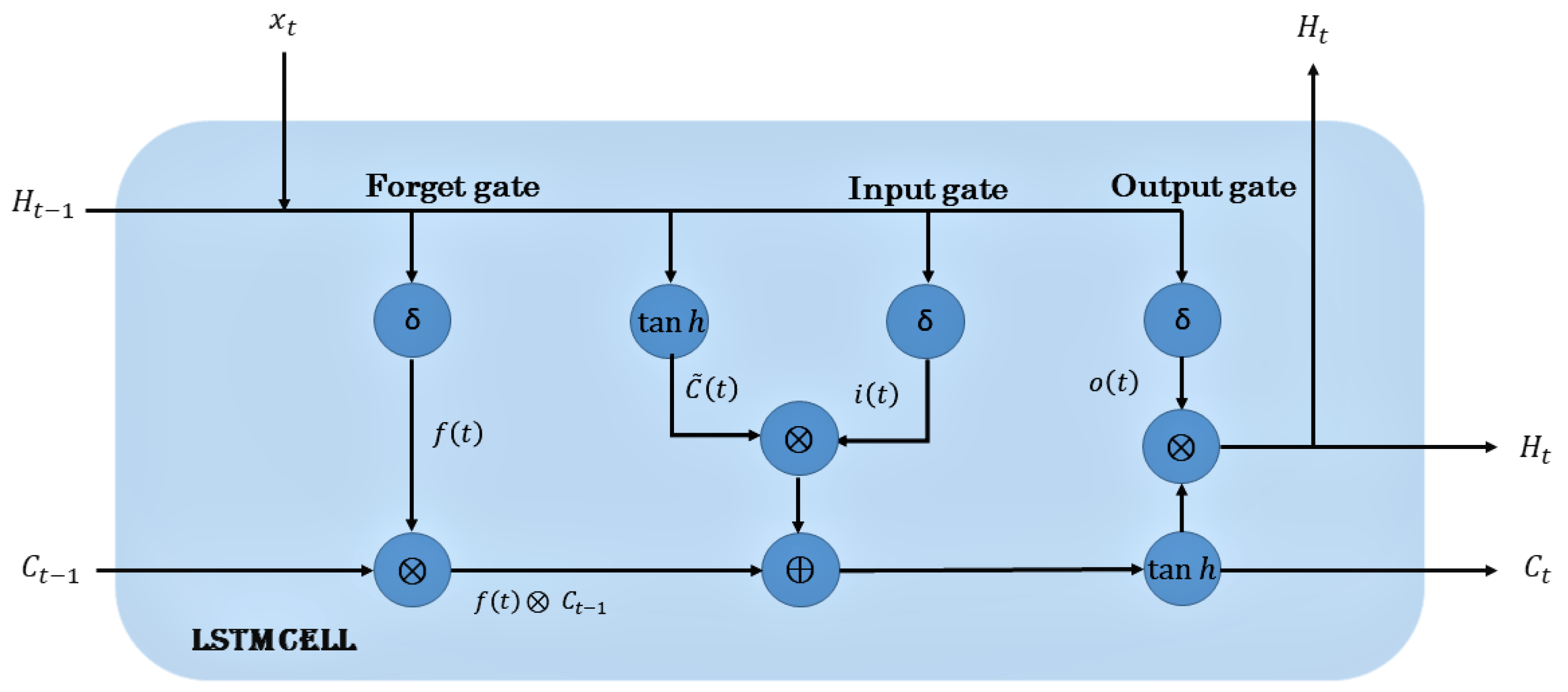
An LSTM [22] network uses cell state, input, output, and forget gates to store long-term dependencies to overcome vanishing gradient problem in typical RNNs and was introduced in 1997 by Hochreiter, S. and Schmidhuber, J. The LSTM processes the data sequentially passing the information as it propagates forward. The operations within LSTM allows it to forget or keep the information. The architecture of LSTM model is shown in Figure 4.

The cell state which is shown as a horizontal line runs through the entire network and has the ability to add or remove the information with the help of gates. The process of the cell state is to carry the information through the sequence processing and theory information from earlier time steps can be carried all the way through the last time step thus reducing the effect of short term memory. As the process goes on, the information is added or removed from the cell states to gate states. Gates decide which information is allowed on the cell state. The first gate that is the forget gate is responsible for learning what information is necessary to keep or forget as they contain sigmoid function. The sigmoid function generates numbers between zero and one, describing how much of each component should be let through. The tanh function generates a new vector, which is added to the state. The cell state is updated based upon the outputs generated from the gates.

The sigmoid function is given as

$$\begin{array}{c}\hfill sigmoid\left(x\right)=\frac{1}{1+e^{-x}}\end{array}$$

(2)

Equations (3)–(8) represent the flow of information at each gate and cell state of LSTM network:

$$f_t=\sigma (W_f·[h_{t-1},x_t]+b_f)$$

(3)

$$i_t=\sigma (W_i·[h_{t-1},x_t]+b_i)$$

(4)

$${\tilde{C}}_t=tanh(W_C·[h_{t-1},x_t]+b_C)$$

(5)

$$C_t=f_t\ast C_{t-1}+i_t\ast {\tilde{C}}_t$$

(6)

$$o_t=\sigma (W_o·[h_{t-1},x_t]+b_o)$$

(7)

$$H_t=o_t\ast tanh\left(C_t\right)$$

(8)

f${}_{\mathrm{t}}$, i${}_{\mathrm{t}}$, and o${}_{\mathrm{t}}$ represent the outputs generated by forget gate, input gate, and the output gate, respectively. W${}_{\mathrm{f}}$, W${}_{\mathrm{i}}$, W${}_{\mathrm{C}}$, and W${}_{\mathrm{o}}$ are the input weights, respectively. b${}_{\mathrm{f}}$, b${}_{\mathrm{i}}$, b${}_{\mathrm{C}}$, and b${}_{\mathrm{o}}$ are bias terms and H${}_{\mathrm{t}}$ is the output of LSTM network.

3.3. Experimental Set-Up

All models were implemented using Python language version 3.6.7, trained and tested on a computer with an Intel Core i7-8700 CPU processor and the speed of 3.20 GHz using 8192 MB RAM with the graphics card GeForce GTX 1080Ti and the operating system is Linux Ubuntu 18.04.4 LTS. The parameters setting for models is discussed in Section 3.3.1 and Section 3.3.2.

3.3.1. XGBoost and LightGBM

To perform extreme gradient tree boosting algorithm, we used standard XGBRegressor from Python package called xgboost version 0.90 and LGBRegressor from lightgbm Python package version 2.1.1 for the implementation of LightGBM model. To get better results from tree-based models, we needed to find best parameters for each model by using customized search approach. The best parameters for XGBoost model are: n_estimators = 70, max_depth = 2, min_child_weight = 1, learning_rate = 0.2, gamma = 0, colsample_bytree = 1, alpha = 10, and objective = reg:squarederror, with all other parameters set to default. For LightGBM, the parameter setting is: learning_rate = 0.1, max_depth = −1, metric = {‘l1’, ‘l2’}, num_leaves = 255, colsample_bytree = 1.0, objective = regression, subsample = 0.6, and seed = 10. Training the model for the best number of iterations while using early stopping patience until 5 epochs to prevent the model from overfitting gives best results at 28 epochs.

3.3.2. Deep Learning Models

To implement recurrent neural networks (RNNs), a high level neural network API called Keras with Tensorflow back end was used. We tried different parameter settings to design each DL model by changing various parameters, such as number of neurons, number of layers, optimizing function, and learning rate, to obtain the best DL model which not only performs well on the train data but also gives good prediction results on the unseen test data. We used 2–4 layers for constructing each RNN model and ran the model by selecting the number of neuron in each layer ranging as 50, 70, 100, or 150 and found that, by using two layers and keeping the number of neurons in each layer as 70, our RNN models give the best performance by minimizing the problem of overfitting and reducing model complexity. To compare RNNs, we used the same number of epochs, batch size, dropout, and loss function. Hyperparameter settings for GRU, LSTM, and BiULSTM were kept the same for comparison. During model construction process, we used dropout [38], which is a common way to prevent overfitting in neural networks. The number of neurons or units in RNN, dropout rate, and other parameters in each layer from top to bottoms are given as:

• No. of cells in each layer: [70, 70]
• dropout rate of 20% has been used in the second layer of these three models.
• Activation Function: ReLU
• Dense layer unit:1

For CNNLSTM model, the parameter settings for each layer from top to bottom are as follows:

• No. of filters in CONV1D layer: 32, Kernel size: 3, stride:1
• Maxpooling layer: Pool size:3
• LSTM layer cells: 32, dropout rate: 30%
• Activation Function: ReLU
• Dense layer unit:1

Each DL model was trained using mini batch size of 32; early stopping [39] technique was also utilized to prevent the model from overfitting. Call backs were used to save best weights for each model. To optimize the models, we used Rmsprop [40], which is an unpublished optimization algorithm introduced by Hinton, G. and designed for neural networks.

Customized search method was adopted to find the best learning rate for DL models, and 0.0001 were observed to be appropriate, while ’mean absolute error’ was used as the loss function to monitor the loss during training process.

3.4. Performance Evaluation for Models

To evaluate the performance of our models, we compared the observed and predicted concentrations of PM${}_{2.5}$ by using four statistical evaluation metrics: (MAE), (RMSE), (R), and (IA). They are given in Equations (9)–(12). In these equations, $y_i$ is the actual PM${}_{2.5}$ concentration, ${\widehat{y}}_i$ represents the predicted PM${}_{2.5}$ concentration, ${\overline{y}}_i$ is the average of observed values, and n is the predicted length of the test set.

$$MAE=\frac{1}{n}\sum _{i=1}^n|y_i-{\widehat{y}}_i|$$

(9)

$$RMSE=\sqrt{\frac{1}{n}\sum _{i=1}^n{(y_i-{\widehat{y}}_i)}^2}$$

(10)

$$R=\frac{{\sum }_{i=1}^n\left({\widehat{y}}_i{y}_i\right)-{\sum }_{i=1}^n{y}_i{\sum }_{i=1}^n{\widehat{y}}_i}{\sqrt{{\sum }_{i=1}^n{y}_i^2-{\left({\sum }_{i=1}^n{y}_i\right)}^2}\sqrt{n{\sum }_{i=1}^n{\widehat{y}}_i^2-{\left({\sum }_{i=1}^n{\widehat{y}}_i\right)}^2}}$$

(11)

$$IA=1-\frac{{\sum }_{i=1}^n\left(\right|y_i-{\widehat{y}}_i{\left|\right)}^2}{{\sum }_{i=1}^n\left(\right|{\widehat{y}}_i-{\overline{y}}_i|+|y_i-{\overline{y}}_i{\left|\right)}^2}$$

(12)

4. Results and Discussions

The first part of this section compares the models’ mean performance with and without including the CMAQ parameters. The second part covers the performance of each model at all sites after including CMAQ features.

4.1. Models’ Average Performance with and without CMAQ Data

Table A1. Models results for MAE (µg/m${}^3$).

Station	XGB	LGBM	GRU	CNNLSTM	BiULSTM	LSTM
S1	3.5075	5.1181	3.5552	3.0690	2.8794	2.7227
S2	4.4512	5.5831	4.3075	3.9067	3.7797	4.1039
S3	3.8301	3.9306	2.9401	3.1936	3.0620	2.8833
S4	4.8643	5.1423	6.2153	5.6867	4.4786	4.3463
S5	4.3136	4.5965	3.7298	4.1776	3.6853	3.5373
S6	4.7885	5.1277	3.4689	4.4370	3.5026	3.7202
S7	4.8895	4.7912	4.0385	4.5583	4.3802	4.4826
S8	4.4692	4.4405	3.5383	3.7830	3.3958	3.2385
Mean	4.3892	4.8413	3.9742	4.1015	3.6455	3.6294

,

Table A2. Models results for RMSE (µg/m${}^3$).

Station	XGB	LGBM	GRU	CNNLSTM	BiULSTM	LSTM
S1	4.7931	7.0001	4.7342	4.1117	4.0190	3.7764
S2	6.000	7.9019	5.8645	5.2749	5.2515	5.6464
S3	5.2909	5.2943	4.0917	4.3874	4.1877	4.0209
S4	6.6399	6.7859	8.5938	7.9804	6.1148	5.9277
S5	5.9015	6.2443	4.8973	5.4912	4.9557	4.729
S6	6.6514	7.0232	4.8105	5.8224	4.9492	4.9591
S7	6.4122	6.3969	5.3319	5.7208	5.6031	5.5942
S8	6.1765	6.1460	4.6637	5.0417	4.6054	4.4277
Mean	5.9832	6.5991	5.3735	5.4788	4.9608	4.8852

,

Table A3. Models results for R.

Station	XGB	LGBM	GRU	CNNLSTM	BiULSTM	LSTM
S1	0.8374	0.8239	0.9065	0.8838	0.8883	0.9093
S2	0.793	0.8189	0.8493	0.8411	0.8524	0.8432
S3	0.8387	0.8374	0.9019	0.8855	0.8994	0.9067
S4	0.7251	0.7117	0.5401	0.6873	0.8018	0.8135
S5	0.8608	0.844	0.9081	0.8911	0.9074	0.9132
S6	0.876	0.8649	0.9365	0.9072	0.9329	0.9386
S7	0.8474	0.8491	0.8994	0.889	0.8986	0.9017
S8	0.8673	0.86854	0.9280	0.9112	0.9284	0.9317
Mean	0.8307	0.8273	0.8587	0.8620	0.8887	0.8947

and

Table A4. Models results for IOA.

Station	XGB	LGBM	GRU	CNNLSTM	BiULSTM	LSTM
S1	0.9050	0.8901	0.9058	0.9271	0.9314	0.9442
S2	0.8745	0.8922	0.8829	0.8984	0.9069	0.89095
S3	0.9074	0.9012	0.9444	0.9368	0.9384	0.9452
S4	0.8384	0.8151	0.5298	0.7122	0.8659	0.8789
S5	0.9191	0.907	0.9434	0.9297	0.9442	0.9507
S6	0.9306	0.9218	0.964	0.9427	0.9611	0.9634
S7	0.9127	0.9155	0.9377	0.9285	0.9379	0.9355
S8	0.9236	0.9250	0.9551	0.9487	0.9284	0.9624
Mean	0.9014	0.8959	0.8829	0.9030	0.9268	0.9339

(see Appendix A) include the details of each model performance at every station before adding CMAQ features.

Table 1. Models’ average MAE values (µg/m${}^3$) with/without CMAQ features.

Features	XGB	LGBM	GRU	CNNLSTM	BiULSTM	LSTM
F${}_{\mathrm{p}}$ + F${}_{\mathrm{m}}$	4.3892	4.8413	3.9742	4.1015	3.6455	3.6294
F${}_{\mathrm{p}}$ + F${}_{\mathrm{m}}$ + F${}_{\mathrm{c}}$	4.3386	4.7792	3.9533	3.9857	3.6246	3.5847

,

Table 2. Models’ average RMSE values (µg/m${}^3$) with/without CMAQ features.

Features	XGB	LGBM	GRU	CNNLSTM	BiULSTM	LSTM
F${}_{\mathrm{p}}$ + F${}_{\mathrm{m}}$	5.9832	6.5991	5.3735	5.4788	4.9608	4.8852
F${}_{\mathrm{p}}$ + F${}_{\mathrm{m}}$ + F${}_{\mathrm{c}}$	5.9037	6.5343	5.3546	5.3643	4.9168	4.8292

,

Table 3. Models’ average R values with/without CMAQ features.

Features	XGB	LGBM	GRU	CNNLSTM	BiULSTM	LSTM
F${}_{\mathrm{p}}$ + F${}_{\mathrm{m}}$	0.8307	0.8273	0.8587	0.8620	0.8887	0.8947
F${}_{\mathrm{p}}$ + F${}_{\mathrm{m}}$ + F${}_{\mathrm{c}}$	0.8350	0.8304	0.8640	0.8668	0.8927	0.8989

and

Table 4. Models’ average IA values with/without CMAQ features.

Features	XGB	LGBM	GRU	CNNLSTM	BiULSTM	LSTM
F${}_{\mathrm{p}}$ + F${}_{\mathrm{m}}$	0.9014	0.8959	0.8829	0.9030	0.9268	0.9339
F${}_{\mathrm{p}}$ + F${}_{\mathrm{m}}$ + F${}_{\mathrm{c}}$	0.9041	0.8992	0.8905	0.9084	0.9334	0.9368

show the average MAE, RMSE, R, and IA values of all stations before and after including CMAQ features. F${}_{\mathrm{p}}$, F${}_{\mathrm{m}}$, and F${}_{\mathrm{c}}$ represent pollutants, meteorological parameters, and CMAQ features, respectively. From the results in Table 1, Table 2, Table 3 and Table 4, it is clear that, by including CMAQ features that are highly correlated with the PM${}_{2.5}$ concentration, each model’s MAE and RMSE values are decreased while their R and IA values are improved, thus improving the models performance.

4.2. Performance of Models after Adding CMAQ Data at All Locations

Figure 5, Figure 6, Figure 7, Figure 8, Figure 9 and Figure 10 show the actual and forecast results for each model. Figure 11 shows the results of all models and the numerical analysis are subsequently provided in

Table 5. Models results for MAE (µg/m${}^3$).

Station	XGB	LGBM	GRU	CNNLSTM	BiULSTM	LSTM
S1	3.3872	5.0846	3.4858	3.2584	2.6409	2.6484
S2	4.2806	5.4585	4.2922	4.1063	4.0045	4.0995
S3	3.7949	3.7964	2.9551	3.1759	3.0464	2.8623
S4	4.7489	5.0793	6.1284	5.0941	4.4651	4.2987
S5	4.3686	4.4039	3.6297	3.9163	3.6814	3.5057
S6	4.7882	5.1493	3.5640	4.1717	3.4768	3.3964
S7	4.9267	4.8347	4.0547	4.3727	4.2379	4.5891
S8	4.4136	4.4271	3.5166	3.7900	3.4439	3.2771
Mean	4.3386	4.7792	3.9533	3.9857	3.6246	3.5847

,

Table 6. Models results for RMSE (µg/m${}^3$).

Station	XGB	LGBM	GRU	CNNLSTM	BiULSTM	LSTM
S1	4.6443	6.8807	5.0399	4.4284	3.9199	3.6984
S2	5.7573	7.7821	9.1054	5.4990	5.2247	5.6022
S3	5.2859	5.1491	4.4978	4.3430	4.0414	3.9562
S4	6.4752	6.8254	9.2188	7.1382	6.1509	5.8684
S5	5.9329	6.0015	4.8898	5.2103	4.8453	4.6836
S6	6.6210	7.0275	5.6119	5.6495	4.9314	4.7032
S7	6.4090	6.4751	5.7920	5.5931	6.0191	5.6939
S8	6.1043	6.1334	5.6282	5.0527	4.4913	4.4278
Mean	5.9037	6.5343	5.3546	5.3643	4.9168	4.8292

,

Table 7. Models results for R.

Station	XGB	LGBM	GRU	CNNLSTM	BiULSTM	LSTM
S1	0.8475	0.8330	0.9008	0.8729	0.9062	0.9155
S2	0.8027	0.8218	0.664	0.8415	0.8527	0.8557
S3	0.8369	0.8457	0.899	0.8908	0.9066	0.9094
S4	0.7402	0.7091	0.5379	0.7191	0.8119	0.827
S5	0.8599	0.8575	0.9099	0.8987	0.9123	0.9151
S6	0.8755	0.8608	0.9262	0.9106	0.9388	0.9328
S7	0.8484	0.8464	0.8957	0.8891	0.8892	0.9036
S8	0.8692	0.8689	0.9102	0.9120	0.9303	0.9324
Mean	0.8350	0.8304	0.8640	0.8668	0.8927	0.8989

and

Table 8. Models results for IA.

Station	XGB	LGBM	GRU	CNNLSTM	BiULSTM	LSTM
S1	0.9116	0.8994	0.885	0.9114	0.9381	0.9465
S2	0.8803	0.8934	0.5761	0.8892	0.9065	0.9006
S3	0.9074	0.9097	0.9281	0.9357	0.9441	0.9472
S4	0.8495	0.8193	0.4937	0.7678	0.8697	0.8863
S5	0.9171	0.9161	0.9433	0.9363	0.949	0.9516
S6	0.9299	0.9186	0.9447	0.9477	0.9616	0.9662
S7	0.9122	0.9124	0.9205	0.9313	0.9232	0.9335
S8	0.9245	0.9249	0.9294	0.9477	0.9617	0.9624
Mean	0.9041	0.8992	0.8905	0.9084	0.9334	0.9368

. In Figure 5, it can be noticed that, at Stations 2 and 4, XGBoost is not predicting the peak values at some points. In Figure 6, LightGBM has difficulty in predicting the actual values, especially at Stations 1, 2, 4 and 7 where it is showing a wide difference between actual and predicted values. Results of GRU are shown in Figure 7, which shows it is unable to predict the real values at Stations 1, 2, and 4. CNNLSTM in Figure 8 is providing good predictions only at Stations 3 and 8, while, at Station 4, its predictions results are deviating from original values. BiULSTM prediction and actual values are drawn in Figure 9. On average, it is showing better results than any other model; however, at Station 4, it is unable to detect the peak values. LSTM prediction results are shown in Figure 10; it gives better results than all models except at Stations 2 and 7, where the BiULSTM model error values are lower. Overall, LSTM is performing well by giving fewer error values and a higher IA.

The MAE, RMSE, R, and IA values for all models after adding CMAQ data are given in Table 5, Table 6, Table 7 and Table 8. Table 5 provides the MAE values for each model. From the experiments, the BiULSTM model for Stations 1, 2, and 7 gives the lowest MAE values; for all other stations, LSTM evaluation results are the best. The average MAE values for all station in the case of LSTM are also the lowest, i.e., 3.5847 µg/m${}^3$, followed by BiULSTM (3.6246 µg/m${}^3$), GRU (3.9533 µg/m${}^3$), CNNLSTM (3.9857 µg/m${}^3$), XGBoost (4.3386 µg/m${}^3$), and LightGBM (4.7792 µg/m${}^3$), in decreasing order. In terms of RMSE provided in Table 6, LSTM gives the lowest scores at every station except for Station 2, where BiULSTM model gives the lowest error value. The average RMSE ranking for models from lowest to highest is: LSTM (4.8292 µg/m${}^3$), BiULSTM (4.9168 µg/m${}^3$), GRU (5.3546 µg/m${}^3$), CNNLSTM (5.3643 µg/m${}^3$), XGBoost (5.9037 µg/m${}^3$), and LightGBM (6.5343 µg/m${}^3$). Values of R are given in Table 7. BiULSTM network shows the highest score at Station 6; however, R values for LSTM for all other stations are highest as compared to other models. The average R scores from highest to lowest are: LSTM (0.8989) > BiULSTM (0.8927) > CNNLSTM (0.8668) > GRU (0.8640) > XGBoost (0.8350) > LightGBM (0.8304). In terms of IA listed in Table 8, BiULSTM network gives the highest value only at Station 2 (0.9065). IA values for LSTM network are the highest at all other stations. The average IA score from highest to lowest are: LSTM (0.9368) > BiULSTM (0.9334) > CNNLSTM (0.9084) > XGBoost (0.9041) > LightGBM (0.8992) > GRU (0.8905).

From the results of our experiments, the MAE and RMSE values of LSTM network are the lowest while correlation coefficient R and IA are the highest, which shows that this model performs well on this dataset. BiULSTM network is the next best after LSTM, considering all metrics of evaluation. There are still the following limitations:

• The observation period for this study is only one year. If more data were provided, the network would have better capability to understand the spatial and temporal dependencies.
• Our networks were trained on past 24 h data to get next 1 h PM${}_{2.5}$ concentration prediction. As the sequence of future hours increases, the efficiency of the network to predict usually drops. In the future, we will try to generate 24–72 h predictions and check the models’ performance.

5. Conclusions and Future Work

In this study, ground base measurements of pollutants, meteorological, and predictive data from CMAQ models are concatenated after analyzing the dependent features that affect the concentration of PM${}_{2.5}$. We estimate the hourly values of PM${}_{2.5}$ concentration by applying various well-known machine learning models. In our network training process, we input these features to ML models in order to get next 1 h prediction, while the past 24 h data are provided. Due to spatial and temporal constraints, each station gives different prediction results, therefore, average evaluation values are calculated for all sites. The results show that a well-optimized LSTM network performs better than any other models used in the study. Although ML models and specifically RNNs have the ability to map temporal features, it is very important to analyze the data first, which is then followed by optimizing the model. The advantages of pollutants forecasting using ML models include:

• The time, effort, and cost to collect and measure the data from ground based stations or from any other sensors are reduced.
• In the case of any defect or failure of measuring equipment or sensors, there would be missing data that can be generated by ML models in limited resources and time using past data.
• As other pollutants such as NO${}_2$, ozone, and PM${}_{10}$ are also correlated with the concentration of PM${}_{2.5}$, ML models can predict their values as well.

In a nutshell, ML models can be applied in the development of forecasting systems, especially in weather and pollutants concentration predictions. In the future, we will try to overcome the limitations discussed in Section 4 to get better forecasting results.