Abstract
Liquid-handling robots are designed to dispense sub-microliter quantities of fluids for applications including laboratory tests. When larger amounts of liquids are involved, sloshing must be considered as a parameter affecting stability, which is of significance for autonomous vehicles. The measurement and quantification of slosh in enclosed volumes poses a challenge to researchers who have traditionally resorted to tracking the air–liquid interface for two-phase flow analysis. There is a need for a simpler method to predict rollover in these applications. In this work, a novel solution to address this problem is proposed in the form of the Zero Moment Point (ZMP) of a dynamic liquid region. Computational experiments of a partially filled, two-dimensional liquid vessel were carried out using the Volume of Fluid (VOF) method in a finite volume based open-source computational fluid dynamics solver. The movement of the air–liquid interface was tracked, while the Center of Mass and the resulting Zero Moment Point were determined from the numerical simulations at each time step. The computational model was validated by comparing the wall pressure and movement of the liquid-free surface to experimentally obtained values. It was concluded that for a dynamic liquid domain, the Zero Moment Point can be instrumental in determining the stability of partially filled containers subjected to sloshing.
1. Introduction
Recent research suggests that in the future humanoid robots will be able to perform tasks that are physically intense as well as technically complex. While humanoids have been configured for clearing heavy solid blocks [1,2], very little attention has been paid to liquid cargo. The presence of partially filled liquid containers such as large gallons, barrels, or cylindrical vessels [3,4] introduces a new parameter of liquid slosh to the problem of humanoid stability. Previous work on liquid-handling robots has been focused on small quantities of fluids with applications in the automation of chemical or biochemical laboratories [5,6], where they are required to dispense a designated amount of reagent, samples, and/or other liquids into a selected container. Recent advancements in liquid-handling robots for small liquid quantities focus on modular and open-source design [7,8], while hydrodynamics of sloshing liquids have been applied to improve microtiter plate assays [9,10]. In small quantities, the presence of liquids does not pose a significant challenge for the stability of a robot. However, when the amount of fluid is comparable to or larger than the mass of the robot, e.g., the transportation of substantial liquid cargo [11,12], maintaining stability becomes a challenge at greater rates of motion, which introduce sloshing.
Ongoing research concerning the stability of load-carrying humanoid robots can be divided into two groups: feedback control systems, which largely ignore the physical parameters of robots and load such as mass, Center of Mass (CoM) and body geometry [13]; and Zero Moment Point (ZMP), which directly deals with all the aforementioned parameters. ZMP is a point where the influence of all forces acting on the mechanism can be replaced by one single force [14]. While the primary use of ZMP is to dynamically balance the robot, considerable advancement has been made in ZMP applications since its discovery. In 2003 Kajita et al. [15] introduced the table cart method to design a ZMP based controller in order to generate walking patterns of biped robots. A preview controller was utilized that in turn used the future ZMP reference. Errors introduced in ZMP determination due to the differences between the table cart and multi-body model were compensated for by the preview control. Guangbin Sun et al. [16] extended previous work on the table cart method to calculate ZMP’s and the vertical displacement/motion of the CoM on uneven ground, providing dynamic balancing on all types of terrains. Using the novel approach of extended ZMP analysis, an Atlas robot was simulated that successfully demonstrated its ability to walk on uneven terrains. More recently, Scianca et al. [17] incorporated a constraint on stability in the formulation of model predictive control system for humanoid gait generation and obtained recursive feasibility conditions guaranteeing the stability of CoM and ZMP dynamics ensuring intrinsically stability.
An exhaustive search for liquid-handling robots involving relatively larger quantities of fluids did not reveal any previous research, providing the impetus for this study. Sloshing in partially filled vessels is an aggressive movement of the agitated quantity of fluid within a container. It produces dynamic forces on the outer walls, thus growing into a principal concern for the operation of the vessel. The standard approaches to resolving sloshing of inviscid and/or incompressible liquids in a partially filled vessels subjected to sway, surge, pitch, and roll motions using differential equations have been covered in the literature, notably by Faltinsen [18] and Ibrahim [19]. Computational fluid dynamics (CFD) is a powerful numerical tool that facilitates the analysis of liquids under dynamic forces and has been used to study sloshing in partially filled containers leading to more accurate results [20,21]. Within CFD, various methods have been used to study sloshing. For instance, smoothed particle hydrodynamics (SPH) was employed by L. Delorme et al. [11] in an experimental and computational study of water sloshing in a partially filled tank under a forced rolling motion. The Arbitrary Lagrangian Eulerian (ALE) approach with finite element methods (FEM) has been used [21] to simulate fluid structure interaction problems for baffled and non-baffled containers. More recent works on sloshing [22,23,24] provide insight into sloshing for computing force on the walls of the vessel; however, they do not comment on its effect on stability.
In the present study, the effect of sloshing is linked with stability by calculating the ZMP of the fluid domain at different fill levels. In order to simulate the sloshing phenomena and obtain the fluid properties required for calculating ZMP, the open source CFD tool OpenFOAM [25] was employed. The numerical description of sloshing in partially filled vessel was validated against experimental data available in literature.
2. Methodology
2.1. Problem Description
The present study aims to determine the ZMP of the fluid region in a partially filled rectangular container subjected to sloshing motion. The experimental work by Souto-Iglesias et al. [26] was utilized to validate the numerical simulation of sloshing motion in the fluid domain. The computational domain consisted of a 1:60 scaled model of a longitudinal section of a 138,000 mm3 tanker hold resulting in a rectangular region of 900 mm breadth and 520 mm height, as shown in Figure 1. Due to the two-dimensional nature of the problem, the front and back faces were not resolved in the numerical simulation.
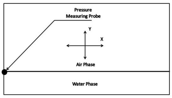
Figure 1.
Computational domain employed in the study.
In the experimental work, the pressure measuring probe was placed on the left boundary at the liquid–air interface (Figure 1) for an 18% fill level, after which the setup was subjected to a ±4° rotation. This necessitates the simulation of not only the two-phase flow but also requires rotation of the mesh. For this purpose, the “Inter-DyMFOAM” solver of OpenFOAM was employed. A uniformly structured mesh with 2400 cells was prepared in the “blockMesh” utility, with an aspect ratio of 1.54074 and a non-orthogonality of 0. A grid independence study was carried out with twice as many cells, which did not indicate a significant effect on the output parameters of Center of Mass and pressure relative to our chosen configuration, as shown in Figure 2; therefore, the initial mesh density was retained for further work.
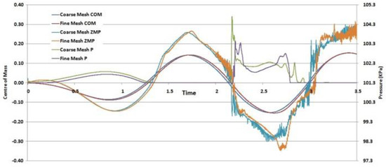
Figure 2.
Grid independence study comparing center of mass (COM), zero moment point (ZMP) and pressure P, for coarse and fine meshes.
2.2. Mathematical Modelling
The mathematical modelling employed in this study had three aspects: the ZMP description of a dynamic liquid region, computationally capturing the dynamics of the air and liquid regions in a domain subjected to periodic motion, and extracting essential information from the computational model for the calculation of ZMP of the dynamic liquid region.
The ZMP [14] methodology describes the stability of bipeds by defining a point where the gravitational force acting on the biped balances the resultant horizontal inertia, which results in no moment along the horizontal plane at the point of contact of the biped with the ground. The ZMP can be calculate using the approach presented by Miomir Vukobratovic [14] along with the table cart method [15,16]. Between these two techniques, the table cart method can be seamlessly integrated to the liquid domain due to its dependence on the Center of Mass.
A basic outline of a liquid tank carrying robot is depicted in Figure 3A, highlighting the CoM and the free surface between the air and liquid regions that is subjected to extreme topological changes during the robot’s motion. Figure 3B shows the cart table description of this robot where a massless table is arranged within a robot and a cart is shown moving on it. Here the cart containing mass “m” at position (x, y) on the table represents the liquid domain of the container, while the table is considered to have the same shape and dimensions of support polygon as that of a robot foot print [27].
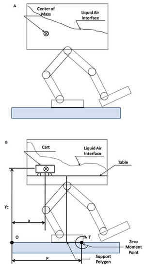
Figure 3.
Liquid carrying robot: (A) simplified model, and (B) table cart description.
The principle of ZMP was adapted from Kajita [15] and Siciliano [27], who employ the following relationship to locate the ZMP with respect to the origin:
where g is the gravitational constant, the location of CoM of the cart along the horizontal axis measured from the origin is x, while is its acceleration and yc is the height of CoM of the cart. For the computation of ZMP for a liquid-carrying robot, the value of yc and x are extracted from CoM, while is obtained from a second order time differencing scheme.
The interDyMFoam (“DyM” stands for “Dynamic Mesh”) solver of OpenFOAM (OF), generally employed to simulate problems involving multiphase flow coupled with moving domains, was modified for this research to calculate the ZMP while solving the three-dimensional Navier–Stokes equations over two fluid domains consisting of incompressible air and water by employing the Volume of Fluid (VOF) approach over a finite volume discretization. The VOF method describes each phase by the fraction αi of the volume of the i’th cell that is occupied by the dispersed phase. The InterDyMFoam solver uses a PIMPLE approach, which combines both the Pressure Implicit with Splitting of Operators (PISO) and the Semi-Implicit Method for Pressure Linked Equations (SIMPLE) algorithms. Its main structure is inherited from the original PISO, but it allows equation under-relaxation to ensure the convergence of all the equations at each time step, as outlined by Jasak [25]. The fluids (air and water) are treated as incompressible, immiscible, and isothermal, while the interface between them is captured using a VOF technique coupled with a moving mesh function. To resolve fluid behavior under dynamic conditions, the conservation of mass and momentum equations are first solved over the liquid and air regions. These are as follows:
where U denotes the velocity, µ denotes the dynamic viscosity, ρ is the density, g is the gravitational acceleration, and t is the time. In order to the capture the air–liquid interface, the VOF method introduces a function α with a value of zero if the mesh cell is completely filled with air and unity if it is completely filled with water [28]. The free surface is formed by the cells containing the value between unity and zero. A special technique can be used to find the derivative of α, keeping in view that it is a step function. These derivatives give the normal direction of quick change in the value of α. Eventually, after determining the normal direction and value of α, a line can be drawn in the boundary cell to show the free surface of the fluid and estimate the interface. The time-dependent governing equation of α is given below:
The Volume of Fluid method in the solver makes use of an artificial compression term ∇·UC α (1 − α) which is added in phase Equation (4). UC is the artificial compressive velocity, and equals to |UC| = min[Cα |U|,max(|U|)]. The fluid density and dynamic viscosity are calculated using following relationships:
where ρwater is the density of water, ρair is the density of air, α is the fluid fraction of water, ρ is the overall density of the control volume, µ is the kinematic viscosity of the overall control volume, and μwater and μair are the kinematic viscosities of water and air, respectively. The term (1 − α) shows that if a cell is α% filled with water then the remaining portion will be filled with air.
The physical properties used in the study include the density of water, ρwater of 998 kg/m3, and dynamic viscosity μwater of 8.94 × 10⁻⁴ kg/(m.s). The density and dynamic viscosity of air are 1.225 kg/m3 and 1.983 × 10⁻⁵ kg/(m.s) respectively, and the surface tension, σ between them is 0.0728 N/m. The frequency of rotation is kept at 2 Hz, while the roll motion amplitude is 4° degree. The upper portion of the container has an atmospheric pressure of 101,000 Pa. The roll center is taken in the middle of the tank (with coordinates of 0 0 −0.225), whereas this study excludes heave and sway motion.
The next phase in the mathematical modelling was the extraction of necessary data from the multiphase description of a dynamic fluid domain. This included the calculation of the CoM and the Cartesian components of its acceleration. The solver was modified to calculate the CoM at each time instant in order to solve Equation (1). For this purpose, let us suppose we have two masses M1 and M2 and their distance from origin X1 and X2 as shown in Figure 4.
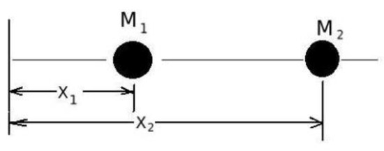
Figure 4.
Center of mass two bodies.
Here, the CoM was between the center of both masses and was calculated by summing the products of the initial masses and distances and dividing this sum with the sum of the masses.
This CoM was calculated for two bodies only for the horizontal distance. While dealing with fluids, CFD gives us several control volumes that are individual masses, and they are three dimensional and can be arranged in two dimensions considering the problem at hand. Equation (7) can be used to obtain the CoM in a three-dimensional space:
In this equation, the COM is obtained in vector format, ri is the position vector of the i’th mass from the origin, and mi is mass of that i’th mass or control volume. In interFoam density is constant, so we can write the mass as ρVi and implement the above equation as in Equation (9).
To implement this condition in openFoam, the following code is added in interStabilityFoam.C:
CoM = sum ( rho ∗ mesh.V() ∗ mesh.C().dimensionedInternalField())/sum( rho ∗ mesh.V());
The spatiotemporal acceleration of the CoM was computed from the following second order numerical difference scheme:
where the equation is using binomial coefficients after the summation sign, x is the location of CoM, h is the time step, and f finds the CoM. Equation (10) provided a numerical estimate of the acceleration, which was implemented in the solver after the start of time loop by first assigning the x, y, and z components of the CoM values calculated previously to scalar variables as follows:
scalar CoMx=CoM.value().x();
scalar CoMy=CoM.value().y();
scalar CoMz=CoM.value().z();
Initially, for the first two steps there was no acceleration based on the backward differencing approach. From the third time step onwards, the acceleration along the x-axis was calculated by the function:
where CoMx3 is the x-coordinate of CoM at the current time step “i”, while CoMx2 and CoMx1 are the x-coordinates of the previous time steps “i−1” and “i−2”, respectively. An if-else loop over a parallel time step was added to the code, in which three time step values of the CoM are stored to calculate acceleration using backward differencing. At every time step “i” the values from the previous time step “i−1” and “i−2” are updated into the parallel time domain. The values of the CoM component are redefined at every time step. The ensuing information was then employed in the estimation of the zero-moment point using Equation (1) as follows:
Ax = (CoMx3 − 2.0 ∗ CoMx2 + CoMx1)/pow((runTime.deltaTValue()),2);
Xzmp = CoMx − ((Ax ∗ CMY)/9.81);
Now, the schematic for the ZMP solver can be drawn, as in Figure 5.
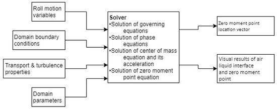
Figure 5.
Outline of solver processes.
In this flow diagram, the roll motion parameters, domain boundary conditions, transport, and turbulence models, as well as domain parameters, are to be specified by the user. The solver solves fluid domain with the governing equations of fluids, i.e., the Navier–Stokes equation, the continuity equation, the phase equation for the air–liquid interface, and the CoM equation to obtain the ZMP. While the Courant number Co should be restricted ~0.25 for the stability of transient simulations in explicit interface capturing solvers, the semi-implicit solver used in the study was unconditionally stable and the value of Co was determined by the solver based on temporal accuracy requirements.
2.3. Test Cases
Seven experimental simulations were carried out in OpenFOAM. First, an experiment with an 18% filled tank was carried out to benchmark the computational method. Subsequent experiments were carried at different fill levels (20%, 30%, 40%, 50%, 60%, 70%, and 80%) in a rectangular tank of the same dimensions. Higher fill levels restrict the physical space available for liquid sloshing so were not significant to the present study.
3. Results and Discussion
The pressure data at the probe from the published results was compared with the pressure at the probe location obtained from the numerical study, as shown in Figure 6, in order to validate computation of air–water multiphase fluid dynamics, after which the ZMP was calculated for the fluid domain to assess stability against tipping over. The maximum deviation between the experimental study and the numerical study was observed to be less than 5.5% in terms of pressure, while the occurrence of the peak pressure pulse showed a maximum of 0.1 s temporal distortion. The numerical implementation of the roll angle had very little deviation from experimental values (<0.01%).
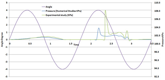
Figure 6.
Pressure comparison (experimental vs. numerical).
This comparison shows that both domains have almost the same angle at same time in the study, leading to very similar pressure perturbations. Different test cases were prepared in this study and pressures extracted for all of them. A comparison of the pressure on the probe at different fill levels is shown in Figure 7. This highlights the behavior of pressure with fill levels indicating that while the occurrence of the peak pressure was over similar roll angles for all fill levels, the magnitude of the pressure peak at the probe position was inversely proportional to the fill level. The only deviation from this inverse relationship was observed between the 18% and the 30% fill level, where the 18% filled tank showed a slightly shorter pressure peak than 30% fill level. This is because the availability of volumetric space allows the fluid to experience greater levels of slosh at lesser fill levels, while at very low fill levels the amount of fluid subjected to slosh is small and unable to generate higher pressure peaks. The maximum value of peak pressure was observed in the 30% filled tank, while tanks that were more than 50% full showed a negligible pressure peak.
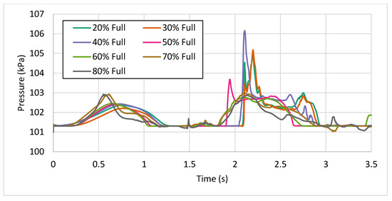
Figure 7.
Pressure curves at different fill levels.
The CoM has a key role in the application of the ZMP. Therefore, after analyzing the pressure it was necessary to observe the behavior of the CoM in relation to the motion of the fluid domain. The change in position of the CoM from the origin with respect to time is shown in Figure 8, along with the pressure sensed by two probes placed on the left- and right-side walls at a distance from the bottom coinciding with the air water interface for an 18% fill level. This comparison shows that pressure is exerted on the walls due to the motion of fluid and, ultimately, the CoM.
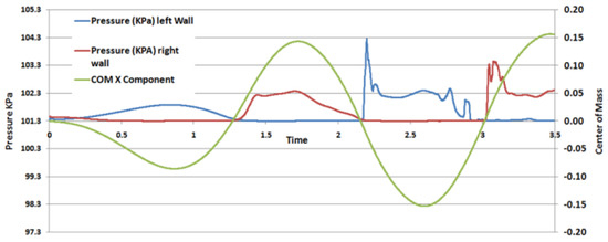
Figure 8.
Center of Mass (CoM) and pressure at the left and right probes.
It was observed that in the first slosh, corresponding to a half roll motion, the CoM did not deviate much, while for the second roll motion the CoM moved a greater value due to a larger amount of liquid slosh. The CoM thus indicates a sinusoidal behavior with increasing amplitude.
We also observed that, as the liquid bulk moved from one side of the container to the other, the pressure sensed by the probe on that side experienced a significant jump. When pressure on left wall increased in first slosh the CoM moved to the left side, giving negative value. After that, the fluid bulk moved towards right side of the tank, due to which the pressure on the left wall probe dropped to zero and right wall probe increased, as shown in Figure 9. Whereas the CoM showed a positive value, the displacement of the CoM was negative in the left half of container and positive in the right half. It was also observed that pressure was higher in the second slosh than that in the first slosh. Thus, the observed behavior of the CoM was in perfect harmony with the roll motion as indicated by the pressures sensed by the two probes.
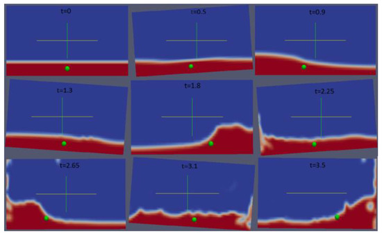
Figure 9.
Center of mass and air–liquid interface.
Next, we summarize the movement of the CoM along with the fluid bulk and the air–liquid interface in Figure 10. The position of the CoM at different time steps can be visually observed in the figure at different angles corresponding to previously described range of roll angles.
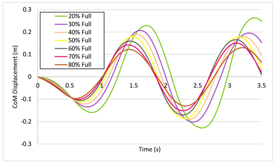
Figure 10.
Center of Mass vs. fill level of container.
The results of the present study highlight the close relation between liquid slosh and CoM, which has hitherto received little attention in the literature due to experimental limitations in determining the CoM. Figure 11 shows the change in behavior of the CoM across the different fill levels of the tanker. This indicates that with the decrease in fill level the CoM moves outwards from the center of domain. Similar to the pressure curves in Figure 8, fill levels greater than 50% exhibited minor changes in the displacement of the CoM, while, contrary to the pressure curve, the maximum displacement was shown by a 18% fill level (instead of 30%). Overall, the two characteristics exhibited similar trends and complemented each other.
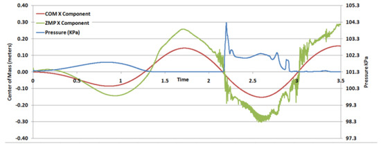
Figure 11.
Zero Moment Point (ZMP), Center of Mass, and pressure comparison.
Using the CoM information and estimating the ZMP according to Equation (1), we plotted the ZMP, the CoM, and the left pressure probe with respect to time for 18% fill level (Figure 11). This showed alternation of the ZMP around the center of domain corresponding to the movement of the fluid bulk. In later roll motions, oscillations were observed in the ZMP location which correspond to sloshing frequencies, while, overall, the Zero Moment Point curve follows the CoM curve (Figure 12).
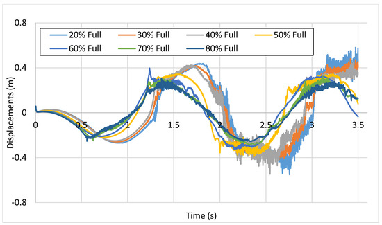
Figure 12.
Displacement of horizontal component of ZMP vs. time at different fill levels.
The evolution of the ZMP across different fill levels is summarized in Figure 12. We observed oscillations in 20%, 30%, and 40% fill levels, while the onset of these oscillations was earliest in the smallest fill level. It can be seen in the case of a 30% fill level that after the onset of oscillations there was slight dampening before it peaked again, while at fill levels of 50% or greater there was no oscillation in the ZMP curve. Hence, we suggest that the ZMP of a dynamic liquid domain can be calculated to estimate its stability, determined by retaining the ZMP within the support polygon as in the present study cases.
4. Conclusions
The stability of dynamic fluid cargo for autonomous vehicles and liquid-handling robots poses a significant hurdle for the advancement of robotics. The indeterministic nature of sloshing liquids that obstruct development of rigorous motion planning has been addressed in this work by a novel approach that incorporates the Zero Moment Point. Computational fluid dynamics (CFD) were employed to capture the displacements of the Center of Mass of a rectangular liquid domain subjected to roll motion by solving the Navier–Stokes equations coupled with the Volume of Fluid (VOF). The computational results were first validated against experimental data prior to the estimation of ZMP. Analysis of the results shows a strong agreement between the fluid’s sloshing motion, the CoM and its ZMP. This enables us to determine the stability of partially filled liquid containers. Further research can be carried out on determining support polygons for complex liquid transport problems involving humanoid robots or autonomous vehicles.
Author Contributions
Conceptualization, M.S. and Y.A.; Methodology, M.U., M.S., Y.A. and E.U.; Software, M.U. and M.S.; Validation, M.U. and M.S.; Investigation, M.U.; Resources, M.S. and E.U.; Data Curation, M.U. and M.S.; Writing—Original Draft Preparation, M.U.; Writing—Review & Editing, M.S.; Supervision, M.S. All authors have read and agreed to the published version of the manuscript.
Funding
This research received no external funding.
Conflicts of Interest
The authors declare no conflict of interest.
References
- Harada, K.; Kajita, S.; Saito, H.; Morisawa, M.; Kanehiro, F.; Fujiwara, K.; Kaneko, K.; Hirukawa, H. A Humanoid Robot Carrying a Heavy Object. In Proceedings of the 2005 IEEE International Conference on Robotics and Automation, Barcelona, Spain, 18–22 April 2005; pp. 1712–1717. [Google Scholar]
- Hirukawa, H. Walking biped humanoids that perform manual labour, Philosophical Transactions of the Royal Society A: Mathematical. Phys. Eng. Sci. 2007, 365, 65–77. [Google Scholar] [CrossRef] [PubMed]
- Kam, L.W.; Gvildys, J. Fluid-structure interaction of tanks with an eccentric core barrel. Comput. Methods Appl. Mech. Eng. 1986, 58, 51–77. [Google Scholar]
- Kargbo, O.; Xue, M.-A.; Zheng, J. Multiphase Sloshing and Interfacial Wave Interaction with a Baffle and a Submersed Block. J. Fluids Eng. 2019, 141. [Google Scholar] [CrossRef]
- Kong, F.; Yuan, L.; Zheng, Y.F.; Chen, W. Automatic Liquid Handling for Life Science:A Critical Review of the Current State of the Art. J. Lab. Autom. 2012, 17, 169–185. [Google Scholar] [CrossRef] [PubMed]
- Lorenz, M.G.O. Liquid-Handling Robotic Workstations for Functional Genomics. J. Assoc. Lab. Autom. 2004, 9, 262–267. [Google Scholar] [CrossRef]
- Faiña, A.; Nejati, B.; Stoy, K. EvoBot: An Open-Source, Modular, Liquid Handling Robot for Scientific Experiments. Appl. Sci. 2020, 10, 814. [Google Scholar] [CrossRef]
- Barthels, F.; Barthels, U.; Schwickert, M.; Schirmeister, T. FINDUS: An Open-Source 3D Printable Liquid-Handling Workstation for Laboratory Automation in Life Sciences. SLAS Technol. Transl. Life Sci. Innov. 2020, 25, 190–199. [Google Scholar] [CrossRef]
- Samad, A.; Khan, A.A.; Sajid, M.; Zahra, R. Assessment of biofilm formation by pseudomonas aeruginosa and hydrodynamic evaluation of microtiter plate assay. J. Pak. Med Assoc. 2019, 69, 666–671. [Google Scholar]
- Zahra, R.; Khan, A.A.; Sajid, M. Hydrodynamic Evaluation of Microtiter Plate Assay Using Computational Fluid Dynamics for Biofilm Formation. In Proceedings of the Asme-Jsme-Ksme 2019 8th Joint Fluids Engineering Conference; American Society of Mechanical Engineers: New York, NY, USA, 2019. [Google Scholar]
- Delorme, L.; Colagrossi, A.; Souto-Iglesias, A.; Zamora-Rodriguez, R.; Botia-Vera, E. A set of canonical problems in sloshing, Part I: Pressure field in forced roll—Comparison between experimental results and SPH. Ocean Eng. 2009, 36, 168–178. [Google Scholar] [CrossRef]
- Liu, D.; Lin, P. Three-dimensional liquid sloshing in a tank with baffles. Ocean Eng. 2009, 36, 202–212. [Google Scholar] [CrossRef]
- Sugihara, T.; Nakamura, Y.; Inoue, H. Real-time humanoid motion generation through ZMP manipulation based on inverted pendulum control. In Proceedings of the 2002 IEEE International Conference on Robotics and Automation (Cat. No.02CH37292), Washington, DC, USA, 11–15 May 2002; Volume 2, pp. 1404–1409. [Google Scholar]
- Vukobratovic, M.; Borovac, B. Zero Moment Point—Thirty Five Years of its Life. Int. J. Hum. Robot. 2004, 1, 157–173. [Google Scholar] [CrossRef]
- Kajita, S.; Kanehiro, F.; Kaneko, K.; Fujiwara, K.; Harada, K.; Yokoi, K.; Hirukawa, H. Biped walking pattern generation by using preview control of zero-moment point. In Proceedings of the 2003 IEEE International Conference on Robotics and Automation (Cat. No.03CH37422), Taipei, Taiwan, 14–19 September 2003; Volume 2, pp. 1620–1626. [Google Scholar]
- Sun, G.; Wang, H.; Lu, Z. A Novel Biped Pattern Generator Based on Extended ZMP and Extended Cart-Table Model. Int. J. Adv. Robot. Syst. 2015, 12, 94. [Google Scholar] [CrossRef]
- Scianca, N.; Simone, D.D.; Lanari, L.; Oriolo, G. MPC for Humanoid Gait Generation: Stability and Feasibility. IEEE Trans. Robot. 2020, 1–18. [Google Scholar] [CrossRef]
- Faltinsen, O.M.; Lagodzinskyi, O.E.; Timokha, A.N. Resonant three-dimensional nonlinear sloshing in a square base basin. Part 5. Three-dimensional non-parametric tank forcing. J. Fluid Mech. 2020, 894, A10. [Google Scholar] [CrossRef]
- Ibrahim, R.A. Recent Advances in Physics of Fluid Parametric Sloshing and Related Problems. J. Fluids Eng. 2015, 137, 090801. [Google Scholar] [CrossRef]
- Sanapala, V.S.; Rajkumar, M.; Velusamy, K.; Patnaik, B.S.V. Numerical simulation of parametric liquid sloshing in a horizontally baffled rectangular container. J. Fluids Struct. 2018, 76, 229–250. [Google Scholar] [CrossRef]
- Ansari, M.; Firouz-Abadi, R.; Ghasemi, M. Two phase modal analysis of nonlinear sloshing in a rectangular container. Ocean Eng. 2011, 38, 1277–1282. [Google Scholar] [CrossRef]
- Boroomand, B.; Bazazzadeh, S.; Zandi, S.M. On the use of Laplace’s equation for pressure and a mesh-free method for 3D simulation of nonlinear sloshing in tanks. Ocean Eng. 2016, 122, 54–67. [Google Scholar] [CrossRef]
- Jäger, M. Fuel Tank Sloshing Simulation Using the Finite Volume Method; Springer: Berlin/Heidelberg, Germany, 2019. [Google Scholar]
- Tang, Y.; Yue, B.; Yan, Y. Improved method for implementing contact angle condition in simulation of liquid sloshing under microgravity. Int. J. Numer. Methods Fluids 2019, 89, 123–142. [Google Scholar] [CrossRef]
- Jasak, H.; Jemcov, A.; Tukovic, Z. OpenFOAM: A C++ library for complex physics simulations, in International workshop on coupled methods in numerical dynamics. In Proceedings of the Ternational Workshop on Coupled Methods in Numerical Dynamics IUC, Dubrovnik, Croatia, 19–21 September 2007; pp. 1–20. [Google Scholar]
- Souto-Iglesias, A.; Botia-Vera, E.; Martín, A.; Pérez-Arribas, F. A set of canonical problems in sloshing. Part 0: Experimental setup and data processing. Ocean Eng. 2011, 38, 1823–1830. [Google Scholar] [CrossRef]
- Siciliano, B.; Khatib, O. Springer Handbook of Robotics; Springer: Berlin/Heidelberg, Germany, 2016. [Google Scholar]
- Hu, Z.Z.; Greaves, D.; Raby, A. Numerical wave tank study of extreme waves and wave-structure interaction using OpenFoam®. Ocean Eng. 2016, 126, 329–342. [Google Scholar] [CrossRef]


© 2020 by the authors. Licensee MDPI, Basel, Switzerland. This article is an open access article distributed under the terms and conditions of the Creative Commons Attribution (CC BY) license (http://creativecommons.org/licenses/by/4.0/).