Abstract
A system for the automatic classification of cardiac sounds can be of great help for doctors in the diagnosis of cardiac diseases. Generally speaking, the main stages of such systems are (i) the pre-processing of the heart sound signal, (ii) the segmentation of the cardiac cycles, (iii) feature extraction and (iv) classification. In this paper, we propose methods for each of these stages. The modified empirical wavelet transform (EWT) and the normalized Shannon average energy are used in pre-processing and automatic segmentation to identify the systolic and diastolic intervals in a heart sound recording; then, six power characteristics are extracted (three for the systole and three for the diastole)—the motivation behind using power features is to achieve a low computational cost to facilitate eventual real-time implementations. Finally, different models of machine learning (support vector machine (SVM), k-nearest neighbor (KNN), random forest and multilayer perceptron) are used to determine the classifier with the best performance. The automatic segmentation method was tested with the heart sounds from the Pascal Challenge database. The results indicated an error (computed as the sum of the differences between manual segmentation labels from the database and the segmentation labels obtained by the proposed algorithm) of 843,440.8 for dataset A and 17,074.1 for dataset B, which are better values than those reported with the state-of-the-art methods. For automatic classification, 805 sample recordings from different databases were used. The best accuracy result was 99.26% using the KNN classifier, with a specificity of 100% and a sensitivity of 98.57%. These results compare favorably with similar works using the state-of-the-art methods.
1. Introduction
According to the World Health Organization, cardiovascular diseases are among the leading causes of death worldwide [1]. An updated report from the American Heart Association on heart disease statistics showed that 31% of deaths worldwide are related to heart disease (17.7 million each year), with the highest rate of mortality in rural areas [1,2]. Typically, people who live in rural areas have limited access to primary care programs for the prevention and early detection of heart conditions [2]. Further exacerbating this situation, medical specialists and equipment, such as cardiologists and echocardiography, are often non-existent in such areas [3]. In this environment, non-specialized medical personnel still have to rely on cardiac auscultation, defined as the listening to and interpretation of cardiac sounds using a stethoscope [4], as the primary method for the screening of heart diseases. However, the effectiveness of auscultation is highly dependent on the skill of the medical practitioner, which in recent years has been discovered to be in decline [5,6,7].
The heart sounds heard by doctors through the stethoscope are due to the noise generated by the opening and closing of the heart valves. A normal heart sound is composed of the S1 sound (generated by the closing of the atrioventricular valve), the S2 sound (generated by the closing of the semilunar valve), the systole (ranging between S1 and S2) and diastole (with a range including S2 and S1 of the next cycle) [4]. In the case of abnormal heart sounds, murmurs usually occur in the systolic or diastolic interval [8]. Different types of heart sound anomalies have been defined, such as aortic stenosis, aortic regurgitation, mitral stenosis, mitral regurgitation and ventricular defect [8]. However, identifying one of these particular conditions from auscultation alone is a very demanding task.
To help with this issue, the development of a system that performs the automatic and reliable classification of normal and abnormal heart sounds is highly desirable. Additionally, this system could have a positive impact in rural areas that do not have specialized personnel and equipment. Generally speaking, a system for the automatic classification of heart sounds is composed of four main stages: a stage of pre-processing, which allows the attenuation of unwanted signals such as external noise or breathing sounds; a segmentation stage, which helps to identify the S1 and S2 sounds in a recording; a stage which is used to extract classification features from segmented cardiac cycles; and a classification stage based on machine learning to decide to which class the signal belongs.
Different methods have been proposed in the state-of-the-art approaches to create an intelligent system that allows for discrimination between normal and abnormal heart sounds. Below is a list of several works related to the pre-processing, segmentation, feature extraction and classification of these signals.
In [9], the envelope of the cardiac signal was calculated from the normalized average Shannon energy (NASE), specifying a threshold to identify the candidate peaks for S1 and S2; then, several criteria were used for the selection of definitive peaks for S1 and S2.
The method used in [10] calculates the Shannon energy of the local spectrum calculated by the S-transform for each sample of the heart sound signal. Finally, the authors extracted features based on the singular value decomposition (SVD) of the matrix S to distinguish between S1 and S2.
The decomposition and reconstruction of cardiac signals with fifth-level discrete wavelets using the frequency bands of the approximation coefficient a4 (0 to 69 Hz) and the detail coefficients d3 (138 to 275 Hz), d4 (69 to 138 Hz) and d5 (34 to 69 Hz) have been used as an alternative to extract normal heart sounds and facilitate the identification of S1 and S2 [11].
In several studies, the decomposition wavelet has been used to reduce signal noise and hidden Markov models (HMM) to segment the signal, considering each segment (i.e., S1, systole, S2 and diastole) as a state [12]. One of the most frequently used segmentation algorithms in the state-of-the-art models was proposed in [13]; this algorithm is based on logistic regression and hidden semi-Markov models and uses electrocardiographic signals (ECG) as a reference to make the annotations of the four segments of a heart cycle (S1, S2, systole and diastole). However, this method fails when the cardiac signal has significant murmurs that are longer than normal heart cycles and there is an irregular sinus rhythm. In [14], the authors present the performance of the algorithm by testing it with different databases of heart sounds and describe the limitations mentioned above.
In [15] a fourth-level, sixth-order Daubechies filter was used on the sound signal. The authors removed all the details at each level and reconstructed the signal using the approximation coefficients. Finally, they used the spectrogram to extract the signal below 195 Hz. In [16], a Butterworth band pass filter with an order of two and cutoff frequencies from 25 to 400 Hz was applied to the signal. The spikes were removed from the signal using a spike removal algorithm, as presented by Schmidt [17]. Subsequently, the authors used a homomorphic filter to extract the envelope of the cardiac signal. In [18], a fifth-order Chebyshev type I low-pass filter with cut-off frequencies of 100 Hz and 882 Hz was applied. Then, the Shannon envelope of the normalized signal was computed. Similarly, in [19], the authors used a sixth-order Butterworth bandpass filter with cut-off frequencies of 25 Hz and 900 Hz and then extracted the signal envelope using Shannon’s average energy.
In general, although all the methods listed above propose different types of filters in their preprocessing stage, they are not yet sufficiently efficient to attenuate unwanted signals (external noise, murmurs) and amplify S1 and S2 sounds; therefore, the segmentation algorithm can easily make errors in the identification of each cardiac cycle. On the other hand, several segmentation algorithms use fixed amplitude thresholds to detect S1 and S2 sounds, but these can fail when these sounds have a low amplitude that does not exceed the stipulated threshold, as well as when some unwanted noise exceeds the threshold. Table 1 summarizes different processing methods proposed in the literature along with their year of publication.

Table 1.
Summary of previous work in the automatic segmentation of heart sounds.
The Physionet and Pascal databases are the most widely used databases for the analysis of heart sounds. Physionet is composed of eight data sets and contains 3153 recordings in total, of which 2488 recordings are labelled as normal and 665 recordings are labelled as abnormal, presenting an imbalance in the data set [20]. The Pascal database is composed of two data sets and contains the following categories: normal (351 recordings), murmur (129 recordings), extra heart sound (65 recordings) and artifact (40 recordings). Unlike Physionet, the manual segmentation of a group of heart sound recordings is specified in this database [21].
On the other hand, different techniques for the extraction of characteristics and machine learning models have been proposed for the automatic classification of heart sounds in order to obtain good accuracy, specificity and sensitivity in the results. Many researchers have worked with features in the time and frequency domain, as well as perceptual-based features. Table 2 shows the results obtained from various authors, specifying the number of cardiac cycles used for the experiment, the segmentation and feature extraction methods and the machine learning (classifier) model.
Table 2.
Summary of the state-of-the-art approaches. N: normal, A: abnormal, T: total, NN: does not specify the data, F: features, A: accuracy, E: specificity, S: sensibility, DWT: discrete wavelet transform, LPC: linear prediction coefficients, SVM: support vector machine, KNN: K-nearest neighbor, RF: random forest, LB: LogitBoost, CSS: cost-sensitive classification, DNN: dense neural network, ANN: artificial neural network.
In [25], 19 Mel-frequency cepstral coefficients (MFCCs) and 24 discrete wavelet transform (DWT) features were extracted from a cardiac cycle. These features were used as inputs to a Support Vector Machine (SVM) model to classify normal and abnormal heart sounds, obtaining an accuracy of 97%.
In [26], the authors extracted a total of 27 features: 13 MFCC features, 10 statistical features and four frequency features. In that work, they used an XgBoost algorithm, obtaining an accuracy of 92.9%. In [27], six linear prediction coefficients (LPC) and 14 MFCCs were extracted for each segment of a cardiac cycle (S1, S2, systole and diastole). These features became the input to three classifiers (SVM, KNN and random forest), obtaining an accuracy of 94.6%. In [30], a total of 90 features were extracted in the time domain, time–frequency and perceptual dimensions. These were used as the input to a two-layer feed forward neural network, achieving 90.1% sensitivity and 93.1% specificity in the validation process, using samples that present high sound quality. In [31], deep convolutional neural networks and MFCCs were used for the recognition of normal and abnormal heart sounds, achieving an overall accuracy of 84.15%.
The experiments in [26,28,32,33,34,35,36,37,40] were performed with the Physionet database [20]. In [32], features were extracted in time, frequency, wavelet and statistics, obtaining a total of 29 features. In the classification stage, a nested set of ensemble algorithms consisting of random forest (RF), LogitBoost (LB) and cost-sensitive classification (CSS) were used, obtaining an overall accuracy of a 80.1%, specificity of 80.6% and sensibility of 79.6%.
Table 1 and Table 2 show different methods used for automatic segmentation and classification of heart sounds, respectively. However, the techniques used in segmentation tend to fail when the sound signal contains murmurs or external noise with amplitude peaks equal or greater than the peaks of the S1 or S2 sounds. As for automatic classification, it tends to require very complex feature extraction and classification models that limit its use in real-time applications due to their high computational cost. Therefore, this article proposes methods to combat these limitations.
This article proposes a robust algorithm that allows the automatic segmentation of normal and abnormal phonocardiogram (PCG) signals, identifying the systolic and diastolic intervals of a recording even in the presence of high-amplitude murmurs. The proposed method uses the modified empirical wavelet transform and normalized average Shannon energy. Additionally, an analysis and classification procedure is proposed to discriminate between normal and abnormal heart sounds, using as a model input the signal power extracted from several sub-segments of the systole and diastole. A total of four classifiers were tested: support vector machine (SVM), K-nearest neighbor (KNN), random forest and multilayer perceptron (MLP).
The rest of this document is organized as follows: Section 2 presents the proposed method for the automatic segmentation of heart sounds; Section 3 presents the proposed method for the feature extraction and classification of segmented heart sounds; Section 4 presents the results for the segmentation and classification of heart sounds compared with the state of the art; and finally, Section 5 presents the discussions and conclusions of the work.
2. Proposed Method for Automatic Segmentation of Heart Sounds
In this method, the algorithm proposed in [41], called empirical wavelet transform (EWT), is studied as a reference in the preprocessing stage of the cardiac signal. The EWT allows the extraction of different components of a signal when designing an appropriate filter bank. The theory of the EWT algorithm is described in detail in [41]. This method has given better results than empirical mode decomposition (EMD), since the latter decomposes the signal in many ways that are difficult to interpret or do not give relevant information [41].
The EWT algorithm has been used as a signal filtering stage in different applications, such as in the processing of voice and movement signals for the classification of Parkinson’s disease severity [42], detection of mechanical failures from vibration signals [43] and in the analysis of geomagnetic signals for the detection of seismic activity [44]. However, this technique demands a high computational cost, since the model can decompose the signal into many components according to the criteria and then chooses the optimal component, and is therefore a non-viable method for a real-time system. Therefore, many researchers have sought ways to apply improvements to the method in order to obtain the desired components in a more effective way, as described in [42,43,44].
In our case, we need to improve the EWT algorithm to extract the S1 and S2 components of the cardiac signal, while attenuating the murmurs or external noises that are present in the original signal. To achieve this, we consider that the frequency range of the S1 and S2 sounds is between 20–200 Hz [45]; therefore, we decided to modify the edge selection method that determines the number of components.
Figure 1 shows the block diagram for the proposed segmentation system. Initially, all the signals taken from the databases are decimated to a sampling frequency of 4 kHz and amplitude-normalized using Equation (1), where X(n) and N denote the original signal and the length in samples of the signal.
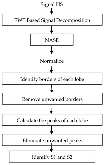
Figure 1.
Block diagram for the proposed segmentation system.
The first stage of the system decomposes the signal into different frequency bands using the modified EWT (mEWT) method. To achieve this, the first step is to identify the maximum value of the Fast Fourier Transform (FFT) of the signal, which is in the range of 20 Hz to 150 Hz. After identifying which frequency belongs to the maximum value, this is taken as the center frequency for a filter with a bandwidth of 40 Hz; that is, if the center frequency is 70 Hz, a bandwidth between 50–90 Hz is established using the EWT method. Thus, we reduce the computational cost by not computing many filters for many different frequency bands and efficiently eliminate unwanted noise.
In Figure 2, a heart sound and its respective FFT are shown. In this example, the maximum amplitude is approximately 60 Hz; therefore, the frequency band is 40–80 Hz, as seen in the green segment (see Figure 2B). Figure 2 also shows four components in order to illustrate the shape of the signal in different frequency ranges, using the adaptive filters of the EWT method. For this example, the low-frequency segment is defined between 1–40 Hz (blue segment, Figure 2C); in the segment from 80 Hz to 350 Hz, some kind of murmur is expected (red segment, Figure 2E); and in the segment of 350 Hz and above, it is expected that high-frequency noises that intervene in the recording can be observed (cyan segment, Figure 2F). It can be seen that in the segment of 40–80 Hz (green segment, Figure 2D), the S1 and S2 sounds have a considerable amplitude that can facilitate their identification.
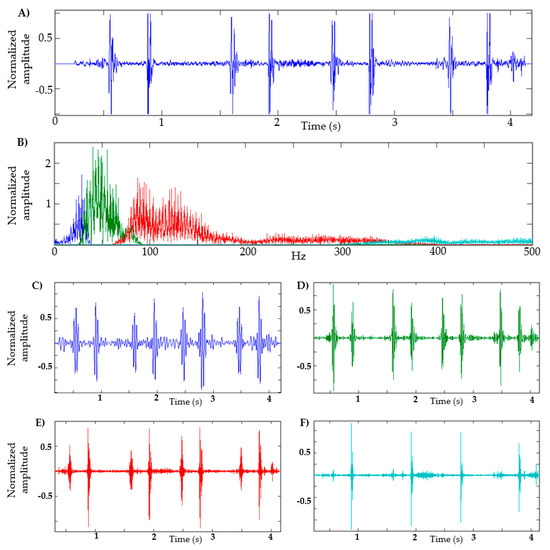
Figure 2.
Decomposition of heart sound using EWT. (A) Heart sound recording; (B) FFT of heart sound with the frequency bands determined; (C) EWT components defined between 1–40 Hz. (D) EWT components defined between 40–80 Hz. (E) EWT components defined between 80–350 Hz. (F) EWT components defined at 350 Hz and above.
A main stage in automatic segmentation is the detection of the envelope of the S1 and S2 segments. Various techniques have been attempted in the literature, such as the absolute value of the signal, quadratic energy, Shannon entropy, Shannon energy and Hilbert transform, among others [46]. In [46], the authors make a comparison of different methods used to calculate the envelope of the PCG signal, with the Shannon energy being the most effective for identifying the S1 and S2 peaks. In [9,10,11], this method is used, obtaining good results in the identification of S1 and S2 segments. The Shannon energy equation is defined as
where x (i) represents the samples of the signal and E is Shannon’s energy.
When calculating the quadratic value of a sample, large oscillations can be generated; the amplitude of the sample increases when the absolute value of the original amplitude is greater than 1 and decreases otherwise. Therefore, it is convenient to use normalized energy, as in the case of the normalized average Shannon energy (NASE) [47], defined as follows:
where is the average value of energy E of the signal, is the standard deviation of energy E of the signal and En is the normalized average Shannon Energy.
After calculating the NASE in the HS signal decomposed by the EWT—that is, that signal that has the S1 and S2 sounds—the negative values are equaled to zero and the signal is normalized. In Figure 3B, the result of an NASE signal of a heart sound recording can be observed.
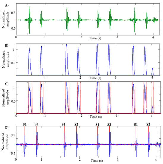
Figure 3.
Stages of segmentation: (A) EWT component: heart sound; (B) NASE of the signal; (C) identification of borders of each lobe; (D) identification of S1 and S2 sounds.
Analyzing the NASE signal, we will proceed to identify the edges of each lobe of the signal; this helps to determine the beginning and the end of the sound S1 or S2. The limits obtained from each lobe are shown in Figure 3C. A problem commonly occurs when there are lobes that are very close to each other; in this case, the lobe that has less energy is eliminated. This process is repeated three times. Lobes of short duration and low amplitude are also eliminated.
Subsequently, the peaks in each lobe are calculated as shown in Figure 3D. Unwanted peaks are removed using the following steps:
- Calculate the average of the intervals between peak (i) and peak (i + 1).
- Eliminate the peaks that belong to an interval less than 0.25 * on average.
- Eliminate the peaks that belong to an interval less than 0.3 * on average.
- Eliminate the peaks that belong to an interval less than 0.4 * on average.
- Eliminate the peaks that belong to an interval less than 0.55 * on average.
There are cases in which the sound of S1 or S2 has a low amplitude and short duration, as seen in Figure 4A. Generally, the methods presented in the state-of-the-art approaches fail in this case. Taking into account the fact that the duration of the cardiac cycle is approximately 0.8 s and the diastolic interval is approximately 0.6 s [48], a condition is established in which the interval between each peak is evaluated, and if in most cases the interval is greater than 650 milliseconds, it can be said that there is a sound (S1 or S2) in that interval. Then, each interval is normalized as shown in Figure 4C. Subsequently, all the previous stages are performed to find sound S1 or S2.
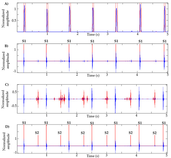
Figure 4.
Segmentation of heart sounds with S1 of low amplitude and short duration. (A) NASE of heart sound; (B) Identification of peaks; (C) Heart sound with normalized intervals; (D) Identification of S1 sounds.
To identify the S1 and S2 sounds in a recording, it is enough to know that the systolic interval is located between S1 and S2, while than the diastolic is located between S2 and S1 of the next cycle. In addition, it is known that the systolic interval is always shorter than the diastolic [48]. With these criteria, it is easy to identify which are the sounds S1 and S2, systole and diastole.
3. Proposed Method for Automatic Classification of Heart Sounds
3.1. Feature Extraction
After the stages of noise reduction (pre-processing) and segmentation, we proceed to the feature extraction in the cardiac cycle. In this stage, the features of the signals that facilitate the classification process are extracted. Many signal processing techniques have been tested in the literature (see Table 2); however, many require a high computational cost for extraction and also extract many features, requiring in turn a complex classification model. Health professionals use different attributes of heart murmurs to achieve their discrimination, the most common of which are their location, duration, pitch and shape [49]. These attributes are related to the different types of murmurs shown in Figure 5 [50].
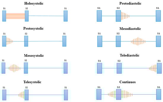
Figure 5.
Types of murmurs according to their location.
Taking as a reference the analysis carried out on the representation of the different types of murmurs shown in Figure 5, we propose the division of the systolic and diastolic interval into three segments and calculate the signal power in each segment, obtaining a total of six characteristics (three in the systole and three in the diastole; see Figure 6). In this way, we try to emulate the attributes (location, duration, pitch and shape) that doctors use to aurally detect some type of heart murmur.
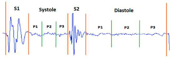
Figure 6.
Distribution of power features for a normal heart sound.
The power of a signal is defined as the amount of energy consumed in a time interval. This calculation is widely used to characterize a signal [51]. In the discrete domain, the power of a signal is given by
The signal is called the power signal when . Figure 6 shows the distribution of the power features.
With this method, it is possible to establish criteria to advance the classification of types of murmurs. For example, if the value of the power P1 of the systole is greater than the P2 and P3 powers, it can be assumed that the type of abnormality is protosystolic.
In this work, this study is not carried out since not all the samples used in the experiment are labeled with the corresponding type of abnormality. Therefore, it is decided to work only on the classification of normal and abnormal sounds and leave the identification of specific anomalies for future work when a suitable training database is available.
3.2. Classification
In this stage, four machine learning models were used to compare their precision, specificity and sensitivity. The models are the support vector machine (SVM), K-nearest neighbors (KNN), random forests (RF) and multilayer perceptron (MLP). These models are selected because they have been widely used in the state-of-the-art approaches (see Table 2) and have given good classification results. The different models used in this work are described below.
- -
- SVM: This classification method, developed by Vladimir Vapnik and his team (Lee et al. 2002), is one of the most used in pattern recognition and binary classification problems, such as for discriminating between normal and abnormal heart sounds. This model is based on constructing a hyperplane that allows the separation of the data into two classes [52].
- -
- KNN: The K-nearest neighbor classifier computes the distance between the data that we want to classify and labeled training data, selecting the nearest neighbors. Based on the neighbor’s category, it is determined to which class the test data belongs [53]. The Euclidean distance is commonly used to determine nearby neighbors for the test data. This model is also suitable for binary classification.
- -
- RF: Random forest is a combination of tree-structured classifiers, where each tree depends on the values of a random vector. To classify an input vector, each tree that belongs to the forest gives a “vote” for classification. Subsequently, the model determines the classification according to the highest number of votes. Random forest is very efficient when used for binary classification on a large number of samples, guaranteeing good specificity and sensitivity in the results. However, it is confusing in terms of its interpretation compared to decision trees [54].
- -
- MLP: The multilayer perceptron (MLP) is a direct-feed artificial neural network and is the most widely used neural network classifier. The MLP has an input layer that takes the characteristics/patterns of the training data, a hidden layer and an output layer with one node per class. The inverse propagation algorithm is used to calculate the weights transported by the network connections. The number of nodes in the hidden layer is determined experimentally [55].
The well-known tool for data mining and machine learning Weka (Knowledge Environment of Waikato University) was used to construct classification models [56]. The power characteristics were used as inputs for the three classifiers (SVM, KNN, RF and MLP). A cross validation of 10 folds was used to evaluate the performance of each classifier.
4. Results
4.1. Results of Automatic Segmentation of Heart Sounds
The heart sound database can be downloaded from the Pascal Classifying Heart Sounds Challenge website [24]. Data have been gathered from two sources: (A) samples acquired through a smartphone using the iStethoscope app and (B) samples acquired in a hospital setting using a DigiScope electronic stethoscope. The database contains the following categories: normal, murmur, extra heart sound and artifact. Table 3 presents in detail the number of recordings and cardiac cycles for the two datasets.
Table 3.
Database of heart sounds: Pascal Challenge. HS: heart sound.
In [24], the results of manual segmentation carried out by experts are presented that serve to evaluate the performance of the segmentation algorithms. The objective of this challenge is to calculate the number of cardiac cycles and identify the S1 and S2 sounds of a recording. Table 4 and Table 5 show the results obtained using dataset A and B respectively, where the evaluation metric is the error that exists between manual segmentation labels provided by the database and those obtained by the proposed method; that is, the difference between the samples corresponding to the S1 and S2 sounds with those detected by the segmentation algorithm. In [24], a spreadsheet is presented to evaluate the error of each sound.
Table 4.
Results of segmentation for dataset A. (HB: heartbeat).
Table 5.
Results of segmentation for dataset B.
Table 6, the results of the total errors shown in [17,18,19,20,21] and the proposed method for datasets A and B are shown. Taking into account that the results presented in [19,20,21] were the best for the Pascal Challenge. Our method obtained a total error of 843,440.8 for dataset A and 17,074.1 for dataset B. These results are the best compared to the state-of-the-art approaches.
Table 6.
Results general of segmentation.
This algorithm was also tested with recordings obtained from Physionet, specifically those signals in which the method in [13] failed, as described in [14]. Figure 7 presents the result of the segmentation in recordings a031, a0112, a0284 and a0352 using the proposed method. In [14] (Figure 4, page 14 of that article), the result of segmentation with these same signals is presented using the method in [13] based on logistic regression and HSMM, with this being one of the most used algorithms in the state of the art. As shown in Figure 7, the proposed algorithm correctly detects the S1 and S2 sounds in each of the recordings.
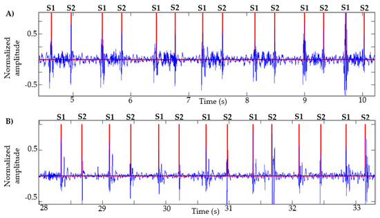
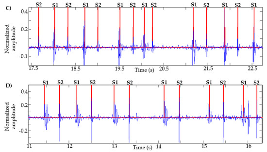
Figure 7.
Examples of segmentation using the proposed method. Heart sound signals for recordings (A) a031, (B) a0112, (C) a0284 and (D) a0352 are taken from the PhysioNet/CinC Challenge 2016, together with the successful segmentations using the proposed algorithm.
4.2. Results of Automatic Classification of Heart Sounds
Accuracy, specificity and sensitivity are the metrics used to evaluate the performance of each classifier. These values were calculated from Equations (5)–(7), respectively, where the values TP (true positive), TN (true negative), FP (false positive) and FN (false negative) are taken from a confusion matrix [57].
- TP: Number of normal heart sounds that were classified as normal.
- TN: number of abnormal heart sounds that were classified as abnormal.
- FP: Number of abnormal heart sounds that were classified as normal.
- FN: Number of normal heart sounds that were classified as abnormal.
This work makes the comparison of models [25,26,27] with the proposed method, since they used characteristics in the domains of time, time–frequency and perceptual domains and techniques used for audio recognition—specifically, the voice. Therefore, different techniques were implemented to extract the characteristics that the authors used in their works. Table 7, Table 8 and Table 9 describe in detail the characteristics used in [25,26,27], respectively. Regarding the classification stage, in [27], the SVM, KNN and random forest algorithms were used; in [25], deep neural networks and SVM were used, with latter showing the best performance; and in [26], the best performance was obtained using the XgBoost algorithm.
Table 7.
Features used in [25].
Table 8.
Features used in [26].
Table 9.
Features used in [27].
In the case of the model in [28], 1D and 2D convolutional neural networks (CNN) were used. In the 1D-CNN model, the authors performed the normalization of 1000 samples for each cardiac signal in order to use it as the input to the model. For the 2D-CNN model, they extracted 12 MFCC features in each 30 ms frame, obtaining a 96 × 12 feature matrix. Table 10 shows the configurations of the 1D-CNN and 2D-CNN model.
Table 10.
Summary of 1D-CNN and 2D-CNN model configurations in [28].
Finally, in the model in [29], the authors used 12.5 s of each recording of heart sounds, making a total of 50,000 samples. Then, they applied a decimation with a factor of eight twice until they obtained a total of 782 samples in each recording. This model used recurrent neural networks, specifically long short-term memory (LSTM). Table 11 shows the model configuration.
Table 11.
Summary of LSTM model configurations in [29].
A total of 805 heart sounds (415 normal and 390 abnormal) from six databases were selected:
- -
- Samples taken from PhysioNet/Computing in Cardiology Challenge 2016 [20].
- -
- Pascal challenge database [21].
- -
- Database of the University of Michigan [58].
- -
- Database of the University of Washington [59].
- -
- Thinklabs database (digital stethoscope) [60].
- -
- 3M database (digital stethoscope) [61].
In the models in [25,26,27], segmentation was performed manually for the identification of the cardiac cycle, S1 and S2 sounds and systolic and diastolic intervals, unlike the proposed method that uses the automatic segmentation method described in Section 2. In the case of the models proposed in [28], normalization was applied to 1000 samples in each cardiac cycle and the MFCC features were calculated. Furthermore, for the model in [29], the decimation process was carried out in each recording, until a total of 782 samples were obtained in each signal.
Table 12 shows the comparison of the accuracy results between the methods in [25,26,27] and the proposed method using the different ML models. Table 13, Table 14 and Table 15 show the results of specificity, sensitivity and the area under the receiver operating characteristic curve (AUC), respectively. Table 16 presents the comparison of the results obtained with the proposed method using the KNN classifier and the models proposed in [28,29].
Table 12.
Results of accuracy between the methods in [25,26,27] and the proposed method.
Table 13.
Results of specificity between the methods in [25,26,27] and the proposed.
Table 14.
Results of sensibility between the methods [25,26,27] and the proposed.
Table 15.
Results of AUC between the methods [25,26,27] and the proposed.
Table 16.
Comparison of results between the methods in [28,29] and the proposed method.
Our method obtained an accuracy of 99.25%, a specificity of 100%, a sensitivity of 98.57% and an AUC of 91.81% using the KNN classifier, which was the best result obtained. Furthermore, with all other classifiers tested, our method ranks at or close to the top, suggesting that the proposed segmentation and feature extraction algorithms are indeed useful, irrespective of the classification model applied on their output.
Finally, Table 17 presents the confusion matrix for each classification model using as inputs the characteristics extracted in the proposed method. It can be seen that, in all cases, a good performance was obtained in the detection of normal heart sounds, taking into account the fact that a 10-fold cross validation was applied.
Table 17.
Confusion matrix of proposed method.
5. Discussions and Conclusions
An algorithm for the automatic segmentation of heart sounds based on EWT and NASE was implemented, obtaining good results in the identification cardiac cycles and their segments (i.e., S1, systole, S2 and diastole) in a recording. The algorithm was tested with two datasets of heart sounds proposed in the Pascal Challenge [21]; the metric used in the challenge consists of the sum of the differences between manual segmentation labels provided in the datasets and the segmentation labels obtained with the automatic segmentation in each recording [21]. The results of the proposed methods compared favorably to methods in the current literature that used the same dataset. The error for dataset A was 843,440.8 and for dataset B was 17,074.1. Additionally, tests were performed with recordings from the Physionet database, obtaining good segmentation performance.
With the help of this system, we can analyze and extract characteristics for each heart cycle segment for the development of a complete system for the automatic classification of heart sounds.
On the other hand, several combinations of features and classifiers have been presented to identify normal and abnormal sounds. The proposed method of feature extraction is based on power values in the systolic and diastolic intervals. Subsequently, four classification models were used: SVM, KNN, random forest and MLP. In addition, the characteristics proposed in [25,26,27] were extracted and the results compared with the proposed method. Similarly, models based on deep learning, such as those used in [28,29], were also implemented and compared with the proposed method.
A classification experiment was carried out using samples obtained from different databases downloaded from the Internet. The best results were obtained with the signal power values calculated in the systole and diastole; the classifier with the best results in accuracy and specificity was KNN with values of 99.25% and 100%, respectively, while the random forest classifier obtained the best result of sensitivity and AUC, with values of 98.8% and 99.62%, respectively.
These results compare favorably with those presented in the state-of-the-art approaches [25,26,27,28,29] (see Table 12, Table 13, Table 14, Table 15 and Table 16); additionally, our experiment used a greater number of testing samples compared to previous works, therefore giving more statistical weight to the results, plus a low computational cost for feature extraction and a small number of characteristics for the classification stage, and the tests were performed together with the proposed automatic segmentation algorithm. In general, the resulting metrics for the classification test are at or close to the top marks in Table 12, Table 13, Table 14, Table 15 and Table 16, for every tested classification model. This can be seen as a strong indication that the proposed segmentation and feature extraction methods are indeed useful irrespective of the classification model that is then applied. This method could potentially be implemented in real-time and guarantees a rapid response with low computational cost.
The main limitation that exists in the proposed method is when the recording of the cardiac signal has ambient noises with a high amplitude, since these noises can be contained in different frequency bands. Therefore, automatic segmentation can identify false positives in the systolic or diastolic interval. Similarly, the power features can vary when the signal has these types of noise and the classifier could in turn be confused regarding whether a heart murmur is present, with the detected murmur actually being an ambient noise.
We are in the construction stage of our own database of heart sounds, with a broad and standardized set of recordings taking into account variables such as the age, sex, height and weight of patients and the diagnostic of the abnormal sound type in collaboration with a cardiologist. Additionally, generative adversarial network models are being developed for the generation of synthetic heart sounds (normal and types of abnormalities), since it is difficult to acquire many samples of a specific type of abnormality. By using this future database, we hope to improve the performance of the classification system and advance the classification of specific types of abnormalities and the automatic segmentation of heart sounds. In the long term, we hope to build a complete real-time automatic system based on the Cloud for the classification of heart sounds that is suitable for telemedicine applications.
Author Contributions
Conceptualization, P.N. and W.S.P.; methodology, P.N. and W.S.P.; software, P.N. and S.G.; validation, P.N., S.G. and W.S.P.; formal analysis, P.N. and W.S.P.; investigation, P.N.; resources, P.N.; data curation, P.N.; writing—original draft preparation, P.N.; writing—review and editing, P.N. and W.S.P.; visualization, P.N.; supervision, W.S.P.; project administration, P.N.; funding acquisition, P.N. and W.S.P. All authors have read and agreed to the published version of the manuscript.
Funding
This research received no external funding.
Conflicts of Interest
The authors declare no conflict of interest.
References
- World Health Organization. A global brief on hypertension. 2013. Available online: http://www.who.int/cardiovascular_diseases/publications/global_brief_hypertension/en/ (accessed on 23 June 2020).
- Benjamin, E.J.; Blaha, M.J.; Chiuve, S.E.; Cushman, M.; Das, S.R.; Deo, R.; De Ferranti, S.D.; Floyd, J.; Fornage, M.; Gillespie, C.; et al. Heart Disease and Stroke Statistics—2017 Update: A Report From the American Heart Association. Circulation 2017, 135, e146–e603. [Google Scholar] [CrossRef] [PubMed]
- Arbelaez, C.; Patino, A. State of emergency medicine in Colombia. Int. J. Emerg. Med. 2015, 8, 9. [Google Scholar] [CrossRef] [PubMed]
- Shank, J. Auscultation Skills: Breath & Heart Sounds, 5th ed.; Lippincott Williams & Wilkins: Philadelphia, PA, USA, 2013. [Google Scholar]
- Alam, U.; Asghar, O.; Khan, S.; Hayat, S.; Malik, R. Cardiac auscultation: An essential clinical skill in decline. Br. J. Cardiol. 2010, 17, 8. [Google Scholar]
- Roelandt, J.R.T.C. The decline of our physical examination skills: Is echocardiography to blame? Eur. Heart J. Cardiovasc. Imag. 2014, 15, 249–252. [Google Scholar] [CrossRef] [PubMed]
- Clark, D.; Ahmed, M.I.; Dell’Italia, L.J.; Fan, P.; McGiffin, D.C. An argument for reviving the disappearing skill of cardiac auscultation. Clevel. Clin. J. Med. 2012, 79, 536–544. [Google Scholar] [CrossRef] [PubMed][Green Version]
- Brown, E.; Leung, T.; Collis, W.; Salmon, A. Heart Sounds Made Easy, 2nd ed.; Churchill Livingstone Elsevier: London, UK, 2008. [Google Scholar]
- Liang, H.; Lukkarinen, S.; Hartimo, I. Heart Sound Segmentation Algorithm Based on Heart Sound Envelolgram. Comput. Cardiol. 1997, 1997, 105–108. [Google Scholar]
- Moukadem, A.; Dieterlen, A.; Hueber, N.; Brandt, C. A robust heart sounds segmentation module based on S-transform. Biomed. Signal Process. Control. 2013, 8, 273–281. [Google Scholar] [CrossRef]
- Huiying, L.; Sakari, L.; Iiro, H. A heart sound segmentation algorithm using wavelet decomposition and reconstruction. In Proceedings of the 19th Annual International Conference of the IEEE Engineering in Medicine and Biology Society. ’Magnificent Milestones and Emerging Opportunities in Medical Engineering’ (Cat. No.97CH36136), Chicago, IL, USA, 30 October–2 November 1997; Volume 4, pp. 1630–1633. [Google Scholar]
- Alexander, B.; Nallathambi, G.; Selvaraj, N. Screening of Heart Sounds Using Hidden Markov and Gammatone Filterbank Models. In Proceedings of the 2018 17th IEEE International Conference on Machine Learning and Applications (ICMLA), Orlando, FL, USA, 17–20 December 2018; pp. 1460–1465. [Google Scholar]
- Springer, D.B.; Tarassenko, L.; Clifford, G.D. Logistic Regression-HSMM-based Heart Sound Segmentation. IEEE Trans. Biomed. Eng. 2015, 63, 1. [Google Scholar] [CrossRef]
- Liu, C.; Springer, D.; Clifford, G.D. Performance of an open-source heart sound segmentation algorithm on eight independent databases. Physiol. Meas. 2017, 38, 1730–1745. [Google Scholar] [CrossRef]
- Deng, Y.; Bentley, P.J. A Robust Heart Sound Segmentation and Classification Algorithm using Wavelet Decomposition and Spectrogram. In Proceedings of the Workshop Classifying Heart Sounds, La Palmam, Canary Islands, 24 April 2012; pp. 1–6. [Google Scholar]
- Mubarak, Q.-U.-A.; Akram, M.U.; Shaukat, A.; Hussain, F.; Khawaja, S.G.; Butt, W.H. Analysis of PCG signals using quality assessment and homomorphic filters for localization and classification of heart sounds. Comput. Methods Programs Biomed. 2018, 164, 143–157. [Google Scholar] [CrossRef]
- Schmidt, S.E.; Holst-Hansen, C.; Graff, C.; Toft, E.; Struijk, J.J. Segmentation of heart sound recordings by a duration-dependent hidden Markov model. Physiol. Meas. 2010, 31, 513–529. [Google Scholar] [CrossRef]
- Gomes, E.F.; Pereira, E. Classifying heart sounds using peak location for segmentation and feature construction. In Proceedings of the Workshop Classifying Heart Sounds, La Palmam, Canary Islands, 24 April 2012; pp. 480–492. [Google Scholar]
- Fatima, C.; Abdelilah, J.; Chafik, N.; Ahmed, H.; Amir, H. Detection and Identification Algorithm of the S1 and S2 Heart Sounds. In Proceedings of the 2016 International Conference on Electrical and Information Technologies (ICEIT), Tangier, Morocco, 4–7 May 2016. [Google Scholar]
- PhysioNet/Computing in Cardiology Challenge. Classification of Normal/Abnormal Heart Sound Recordings. Available online: https://www.physionet.org/challenge/2016/ (accessed on 31 May 2018).
- Bentley, P.; Nordehn, G.; Coimbra, M.; Mannor, S.; Getz, R. Classifying Heart Sounds Callenge [online]. Available online: http://www.peterjbentley.com/heartchallenge/#downloads. (accessed on 3 May 2018).
- Renna, F.; Oliveira, J.H.; Coimbra, M. Deep Convolutional Neural Networks for Heart Sound Segmentation. IEEE J. Biomed. Heal. Inform. 2019, 23, 2435–2445. [Google Scholar] [CrossRef] [PubMed]
- Bently, P.J. “Abstract”. In Proceedings of the Workshop Classifying Heart Sounds, La Palmam, Canary Islands, 24 April 2012. [Google Scholar]
- Oliveira, J.; Renna, F.; Mantadelis, T.; Coimbra, M. Adaptive Sojourn Time HSMM for Heart Sound Segmentation. IEEE J. Biomed. Heal. Inform. 2018, 23, 642–649. [Google Scholar] [CrossRef] [PubMed]
- Yaseen; Son, G.-Y.; Kwon, S. Classification of Heart Sound Signal Using Multiple Features. Appl. Sci. 2018, 8, 2344. [Google Scholar] [CrossRef]
- Arora, V.; Leekha, R.; Singh, R.; Chana, I. Heart sound classification using machine learning and phonocardiogram. Mod. Phys. Lett. B 2019, 33. [Google Scholar] [CrossRef]
- Narvaez, P.; Vera, K.; Bedoya, N.; Percybrooks, W.S. Classification of heart sounds using linear prediction coefficients and mel-frequency cepstral coefficients as acoustic features. In Proceedings of the 2017 IEEE Colombian Conference on Communications and Computing (COLCOM), Cartagena, Colombia, 16–18 August 2017; pp. 1–6. [Google Scholar]
- Noman, F.; Ting, C.-M.; Salleh, S.-H.; Ombao, H. Short-segment Heart Sound Classification Using an Ensemble of Deep Convolutional Neural Networks. In Proceedings of the ICASSP 2019—2019 IEEE International Conference on Acoustics, Speech and Signal Processing (ICASSP), Brighton, UK, 12–17 May 2019; pp. 1318–1322. [Google Scholar]
- Raza, A.; Mehmood, A.; Ullah, S.; Ahmad, M.; Choi, G.S.; On, B.-W. Heartbeat Sound Signal Classification Using Deep Learning. Sensors 2019, 19, 4819. [Google Scholar] [CrossRef] [PubMed]
- Abdollahpur, M.; Ghaffari, A.; Ghiasi, S.; Mollakazemi, M.J. Detection of pathological heart sounds. Physiol. Meas. 2017, 38, 1616–1630. [Google Scholar] [CrossRef]
- Maknickas, V.; Maknickas, A. Recognition of normal–abnormal phonocardiographic signals using deep convolutional neural networks and mel-frequency spectral coefficients. Physiol. Meas. 2017, 38, 1671–1684. [Google Scholar] [CrossRef]
- Homsi, M.N.; Warrick, P. Ensemble methods with outliers for phonocardiogram classification. Physiol. Meas. 2017, 38, 1631–1644. [Google Scholar] [CrossRef]
- Plesinger, F.; Viscor, I.; Halamek, J.; Jurco, J.; Jurak, P. Heart sounds analysis using probability assessment. Physiol. Meas. 2017, 38, 1685–1700. [Google Scholar] [CrossRef]
- Meintjes, A.; Lowe, A.; Legget, M. Fundamental Heart Sound Classification using the Continuous Wavelet Transform and Convolutional Neural Networks. In Proceedings of the 2018 40th Annual International Conference of the IEEE Engineering in Medicine and Biology Society (EMBC), Honolulu, HI, USA, 18–21 July 2018; pp. 409–412. [Google Scholar]
- Nogueira, D.M.; Ferreira, C.A.; Gomes, E.; Jorge, A.M. Classifying Heart Sounds Using Images of Motifs, MFCC and Temporal Features. J. Med Syst. 2019, 43, 168. [Google Scholar] [CrossRef] [PubMed]
- Kay, E.; Agarwal, A. DropConnected neural networks trained on time-frequency and inter-beat features for classifying heart sounds. Physiol. Meas. 2017, 38, 1645–1657. [Google Scholar] [CrossRef] [PubMed]
- Li, L.; Wang, X.; Du, X.; Liu, Y.; Liu, C.; Qin, C.; Li, Y. Classification of heart sound signals with BP neural network and logistic regression. 2017 Chin. Autom. Congress (CAC) 2017, 7380–7383. [Google Scholar] [CrossRef]
- Hamidi, M.; Ghassemian, H.; Imani, M. Classification of heart sound signal using curve fitting and fractal dimension. Biomed. Signal Process. Control. 2018, 39, 351–359. [Google Scholar] [CrossRef]
- Juniati, D.; Khotimah, C.; Wardani, D.E.K.; Budayasa, I.K. Fractal dimension to classify the heart sound recordings with KNN and fuzzy c-mean clustering methods. J. Phys. Conf. Ser. 2018, 953, 12202. [Google Scholar] [CrossRef]
- Zhang, W.; Han, J.; Deng, S. Heart sound classification based on scaled spectrogram and tensor decomposition. Expert Syst. Appl. 2017, 84, 220–231. [Google Scholar] [CrossRef]
- Gilles, J. Empirical Wavelet Transform. IEEE Trans. Signal Process. 2013, 61, 3999–4010. [Google Scholar] [CrossRef]
- Oung, Q.W.; Muthusamy, H.; Basah, S.N.; Lee, H.; Vijean, V. Empirical Wavelet Transform Based Features for Classification of Parkinson’s Disease Severity. J. Med. Syst. 2017, 42, 29. [Google Scholar] [CrossRef]
- Qin, C.; Wang, D.; Xu, Z.; Tang, G. Improved Empirical Wavelet Transform for Compound Weak Bearing Fault Diagnosis with Acoustic Signals. Appl. Sci. 2020, 10, 682. [Google Scholar] [CrossRef]
- Alegria, O.C.; Valtierra-Rodriguez, M.; Amezquita-Sanchez, J.P.; Millan-Almaraz, J.R.; Rodriguez, L.M.; Moctezuma, A.M.; Dominguez-Gonzalez, A.; Cruz-Abeyro, J.A. Empirical Wavelet Transform-based Detection of Anomalies in ULF Geomagnetic Signals Associated to Seismic Events with a Fuzzy Logic-based System for Automatic Diagnosis. Wavelet Transf. Some Real World Appl. 2015. [Google Scholar] [CrossRef]
- Debbal, S.M.; Bereksi-Reguig, F. Computerized heart sounds analysis. Comput. Boil. Med. 2008, 38, 263–280. [Google Scholar] [CrossRef] [PubMed]
- Choi, S.; Jiang, Z. Comparison of envelope extraction algorithms for cardiac sound signal segmentation. Expert Syst. Appl. 2008, 34, 1056–1069. [Google Scholar] [CrossRef]
- Martínez-Alajarín, J.; Merino, R.R. Efficient method for events detection in phonocardiographic signals. Microtechnol. New Millenn. 2005, 5839, 398–409. [Google Scholar] [CrossRef]
- Deshpande, N. Assessment of Systolic and Diastolic Cycle Duration from Speech Analysis in the State of Anger and Fear; Academy and Industry Research Collaboration Center (AIRCC): Basel, Switzerland, 2012. [Google Scholar]
- Etoom, Y.; Ratnapalan, S. Evaluation of Children with Heart Murmurs. Clin. Pediatr. 2013, 53, 111–117. [Google Scholar] [CrossRef] [PubMed]
- Johnson, W.; Moller, J. Pediatric Cardiology: The Essential Pocket Guide; Wiley-Blackwell: Hoboken, NJ, USA, 2008. [Google Scholar]
- Gordon, E. Signal and Linear System Analysis; Allied Publishers Limited: New Delhi, India, 1994; p. 386. [Google Scholar]
- Wang, L. Support Vector Machines: Theory and Applications; Springer: Berlin/Heidelberg, Germany, 2005. [Google Scholar]
- Rajaguru, H.; Kumar, S. KNN Classifier and K-Means Clustering for Robust Classification of Epilepsy from EEG Signals: A Detailed Analysis; Anchor Academic Publishing: Hamburg, Germany, 2017. [Google Scholar]
- Sullivan, W. Decision Tree and Random Forest: Machine Learning and Algorithms: The Future Is Here! CreateSpace Independent Publishing Platform: Scotts Valley, CA, USA, 2018. [Google Scholar]
- Haikyn, S. Neural Networks and Learning Machines, 3rd ed.; Prentice Hall: Upper Saddle River, NJ, USA, 2009. [Google Scholar]
- Johnson, E.M.; Cowie, B.; De Lange, W.S.P.; Falloon, G.; Hight, C.; Khoo, E. Adoption of innovative e-learning support for teaching: A multiple case study at the University of Waikato. Australas. J. Educ. Technol. 2011, 27. [Google Scholar] [CrossRef]
- Zhu, W.; Zen, N.; Wang, N. Sensitivity, Specificity, Accuracy, Associated Confidence Interval and ROC Analysis with Practical SAS® Implementations. North East SAS Users Group Health Care Life Sci. 2010, 19, 67. [Google Scholar]
- University of Michigan. Heart Sound and Murmur Library. Available online: https://open.umich.edu/find/open-educational-resources/medical/heart-sound-murmur-library (accessed on 31 May 2018).
- University of Washington. Heart sound and murmur. Available online: https://depts.washington.edu/physdx/heart/demo.html (accessed on 31 May 2018).
- Thinklabs. Heart Sounds Library. Available online: http://www.thinklabs.com/heart-sounds (accessed on 31 May 2018).
- Littmann Stethoscope. Heart Sounds Library. Available online: http://solutions.3mae.ae/wps/portal/3M/en_AE/3M-Littmann-EMEA/stethoscope/littmann-learning-institute/heart-lung-sounds/ (accessed on 31 May 2018).


© 2020 by the authors. Licensee MDPI, Basel, Switzerland. This article is an open access article distributed under the terms and conditions of the Creative Commons Attribution (CC BY) license (http://creativecommons.org/licenses/by/4.0/).