1. Introduction
A liquid sample can be classified using physical properties, such as concentration, color, boiling temperature, and fusion point. In the case of concentration, this can be defined as the amount of solute mass in the total volume of a solution [
1]. There are many methods and tools for the estimation of concentrations in liquid samples; however, most of them are invasive and destructive [
2,
3,
4]. A technique that is able to perform measurements of concentration differences with high accuracy, in a non-invasive and non-destructive way, is digital holographic interferometry (DHI) [
5].
DHI is a high precision, non-contact, non-invasive, non-destructive, and full-field optical metrology technique [
6,
7]. DHI is able to measure, with a very high sensitivity, variations in the physical properties of phase objects (i.e., a liquid sample in a glass container can be considered as a phase object), based on the comparison of wavefronts recorded as holograms at different instants in times or states of an object [
8,
9]. The holograms are recorded by an image sensor, and saved on a computer; then, a reconstruction process can be performed using numerical methods [
10,
11,
12]. The phase difference extracted from reconstructed object images is wrapped from −π to π. The accuracy of the DHI depends on the accuracy with which the phase difference is estimated, which is usually noisy and wrapped [
13]. However, phase unwrapping methods require a robust algorithm [
14,
15,
16,
17]. In addition, phase unwrapping methods have a trade-off between the computational cost and accuracy, i.e., a high accuracy method requires more computational time [
18].
The growth of new computer vision and open-source technologies can improve the trade-off between computational cost and accuracy in phase difference estimation. A new promising technology is the convolutional neural network (CNN). CNNs are mathematical algorithms that mimic the functioning of the mammalian visual cortex using advanced operation blocks, and several layers of neurons, due to the ability to approximate any continuous function accurately [
19]. CNNs have been applied to multiple tasks, including image classification, object detection, object tracking, and scene labeling [
20,
21,
22,
23,
24,
25,
26].
Specifically for the optical metrology techniques, CNNs have been applied as a phase demodulation from a single fringe pattern in projection profilometry [
27], as a phase and amplitude reconstructor from a single hologram intensity pattern in holography [
28], as an estimator of depth position without multiple diffraction calculations in digital holography [
29], and as an optical fringe pattern denoising method in interferometry [
30]. CNNs have also been applied in digital holographic interferometry, including new phase unwrapping methods, e.g., Spoorthi et al. [
31] proposed a phase unwrapping method using the wrapped phase as input and wrap-count as a semantic label, Zhang et al. [
32] presented a phase unwrapping method based on a semantic segmentation algorithm, and Zhang et al. [
33] generated the unwrapped phase from the combination of a denoised wrapped phase and a corrected integral multiple.
Therefore, in order to improve the calculation efficiency and simplify the procedures of phase difference estimation, the aim of this research was to implement open sources and artificially intelligent technologies for DHI in liquid samples. This research proposes to develop a new method that does not need phase unwrapping to estimate concentrations with high sensitivity, high accuracy, and with a low computational cost.
2. Materials and Methods
2.1. Experimental Setup
The optical system for concentration measurements was based on DHI. The principles and mathematical equations of DHI are well known in the literature [
5,
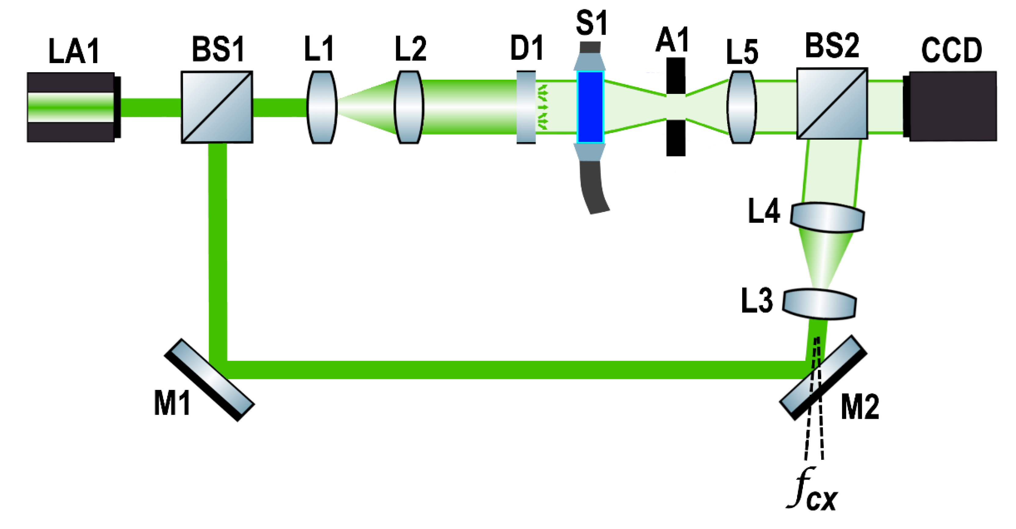
6]. In DHI, phase difference maps were obtained from the correlation between two holograms. The experimental setup we used to record the holograms is shown in
Figure 1. The optical system had a He-Ne laser light
LA1 (CrystaLaser, Reno, NV, USA) with a peak wavelength of λ = 543 nm, and with a maximum output power of 15 mW. The laser beam was divided into two beams by a beam splitter
BS1. One beam (object beam) was sent to the
L1 and
L2 lenses to be expanded and collimated, respectively. Then, the object beam was scattered by a diffuser
D1, and passed through a common glass tube that contained the liquid sample
S1 to be analyzed.
The object beam passed through a rectangular aperture A1 and was collected by a positive lens L5. Then, it was sent to a cubic beam splitter BS2 that was placed in front of an 8-bit charge-coupled device camera (CCD) (Pixelink, Rochester, NY, USA). In addition, the liquid sample with respect to the acquisition camera had a distance of 25 cm. Otherwise, the reference beam was reflected by the M1 and M2 mirrors. Later, the reference beam was sent to the L3 and L4 lenses to be expanded and collimated, and then, the output beam was sent to BS2 where it could interfere with the object beam, which was right in front of the CCD camera.
A small angle was introduced between the object and the reference beam on the Mach–Zehnder configuration to achieve the off-axis holography geometry. The CCD was a monochromatic sensor with 1280 × 1024 pixels (1.3 MP) with an 8-bit dynamic range. The pixel size was 5.2 μm. The holograms were continuously recorded at 13 fps, while the liquid sample passed through the glass tube at a rate of 12 mL/min. This allowed us to create a large image dataset by recording 13 different holograms per second. The liquid sample was continuously injected by a syringe Infusion Pump KDS 200 (KD Scientific Inc., Holliston, MA, USA).
2.2. Phase Difference Images
Seven liquid samples were created by mixing 1 liter of distiller water with various masses of NaCl. The different masses of NaCl used are shown in
Table 1.
In order to measure the concentration difference between two liquid samples, two holograms were recorded at different moments or states. A hologram is obtained from a wave-front. The wave-front coming from certain liquid sample is represented as:
where
is the amplitude,
is the phase of the wave-front, and
are the rectangular coordinates of the recording sensor plane.
Then, a second hologram was obtained from a wave-front coming from another liquid sample or after slightly modifying the concentration of the liquid sample. The new wave-front is represented as:
where
is the new phase that indicates a change in the optical path length, i.e.,
.
The procedure continued with the calculation of the phase difference from the individual phase terms
. A phase term depends on the transverse distances and the refractive index of the liquid mixture inside a glass tube. The refractive index difference is related to the change of concentration (
CON) and the temperature (T) between liquid samples. In the case of aqueous salt mixtures, the liquid samples have a linear relationship between the refractive index and concentration (
CON), which is considered to be constant at 1.71 × 10
−3 at a temperature of 20 °C. Therefore, the concentration difference between two liquid samples can be described as [
5]:
where
,
is the wavelength,
and
are the concentration values of two liquid samples, and
is the inner transversal distance of the glass tube.
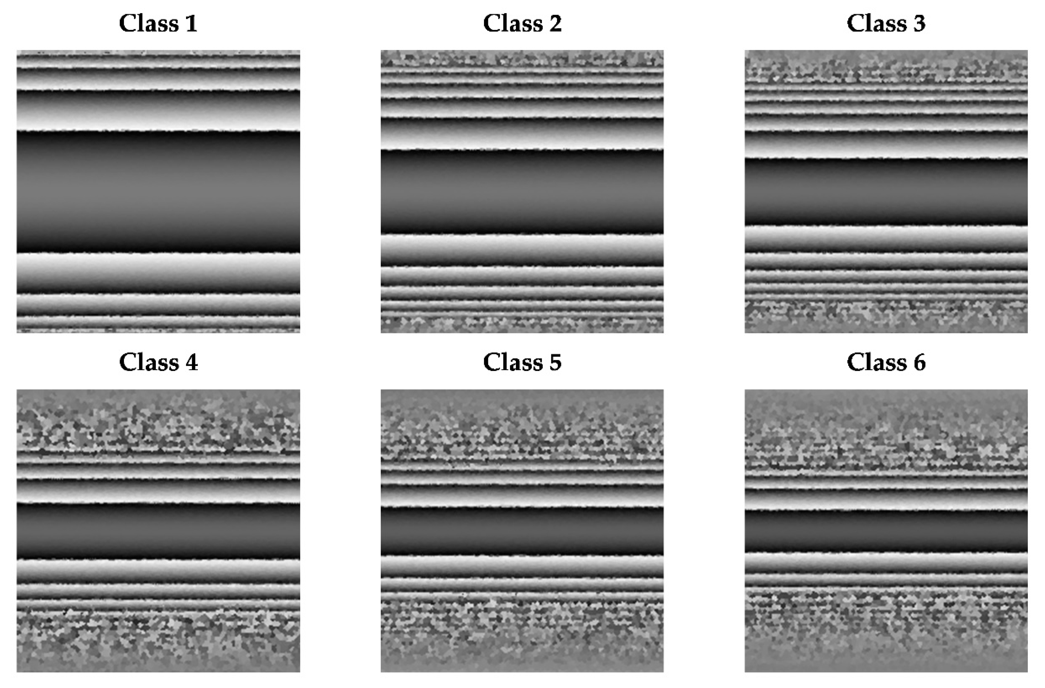
Therefore, the wrapped phase difference images were obtained from the difference between two holograms with different concentrations. The wrapped phase difference images were obtained from the difference between the different samples and the sample with only distilled water (0 g of NaCl), which did not require special preparation. In addition, six classes were created with different concentrations, and they are shown in
Table 2. The wrapped phase difference images for each class are shown in
Figure 2.
2.3. Proposed Method
A simple and highly modularized network architecture for image classification is ResNeXt [
34]. ResNeXt is an improvement of a previous version of ResNet due to its cardinality of 32. This next dimension is known as cardinality. A high cardinality value is a more effective way of gaining accuracy in image classifications. That is to say, ResNeXt is built by the repetition of building blocks that add a set of transformations with the same topology, which allows for greater accuracy [
35]. ResNeXt architecture currently has the lowest Top-1 and Top-5 errors among Torchvision package models [
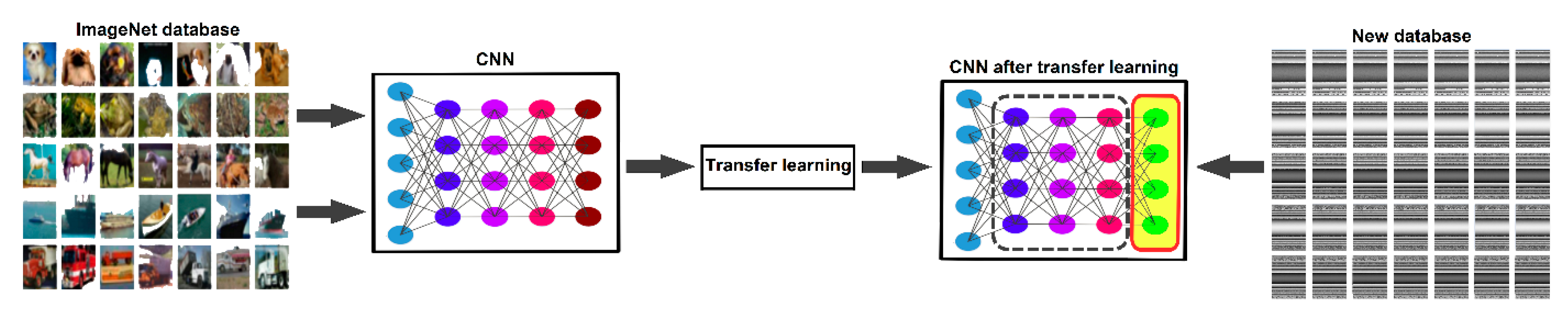
36]. The input size for ResNeXt is 224 × 224 RGB images. Therefore, the characteristics of the ResNeXt model with transfer learning (TL) principles are ideal for use in this research. The main principle of TL is that a CNN model that has been previously trained for a certain task is reused, and trained again to learn a new task. This is possible by modifying the last fully connected layer according to the new number of classes to classify in the new task, and using the process of fine-tuning, which essentially retrains the whole model by unfreezing the convolutional base layers, and allows the weight and bias to be recalculated (updating all of the model parameters).
Figure 3 shows the TL process in a CNN, where the last fully connected layer was changed, from classifying general images to classifying the interferogram dataset collected in this research.
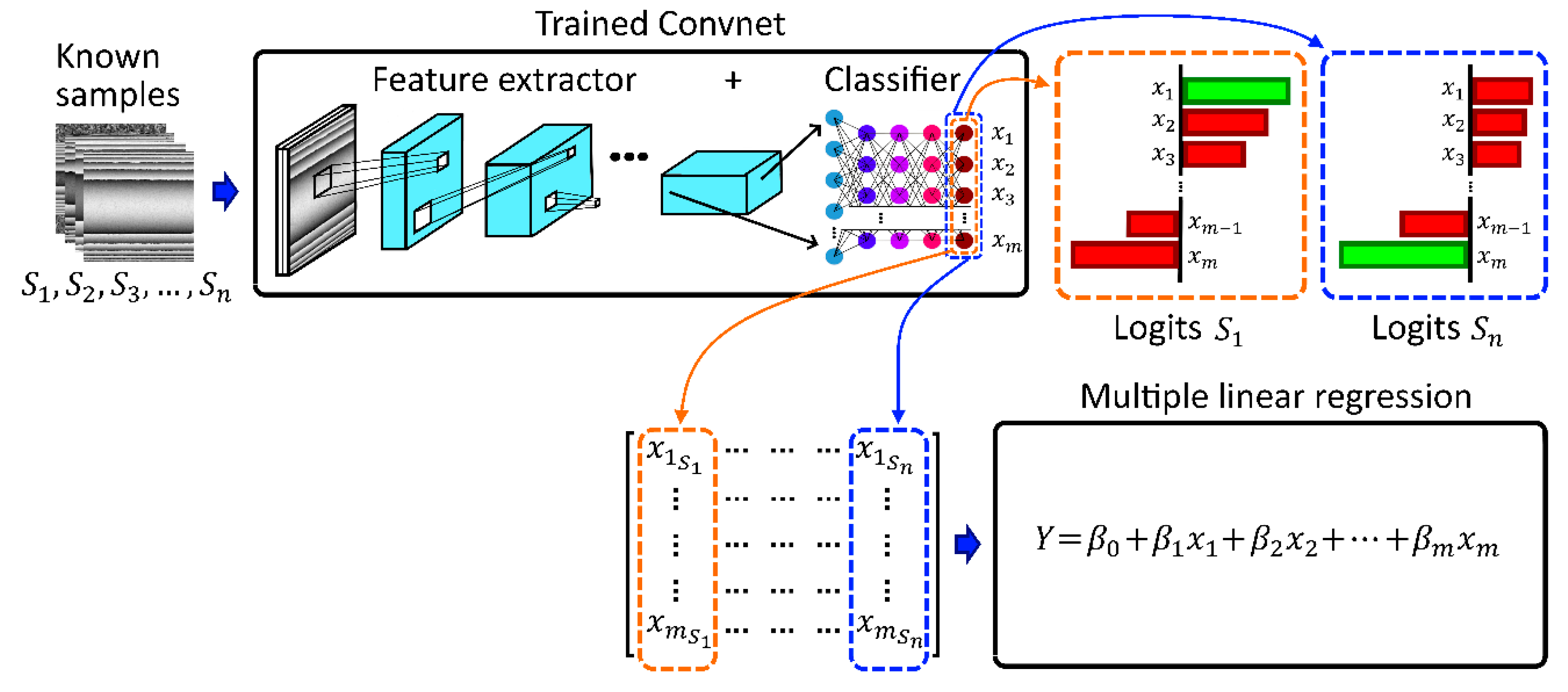
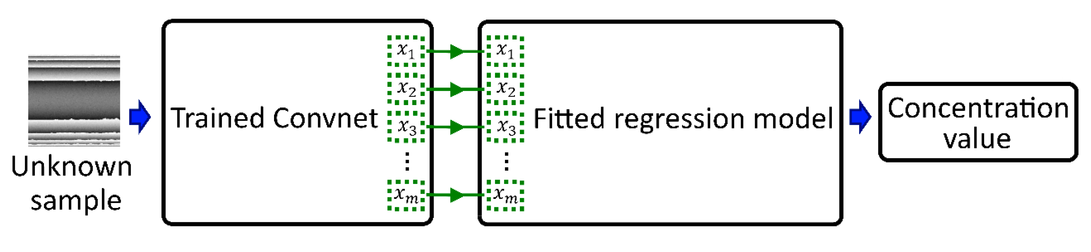
In this research, a ResNeXt model was used to extract implicit information from a dataset and to then use the extracted information to create a feature vector. This feature vector was used to fit a multiple linear regression (Regressor) to predict the concentration measurements from wrapped phase images. The final layer in the ResNeXt model was the logits layer, which returns raw probability values in a feature vector. The Regressor was fitted with the feature vector or logits vector, and an equation was made. The equation relates the feature vector, obtained from the training dataset used to fit the Regressor, with a new feature vector obtained from a new image.
Figure 4 shows the generation of the multiple linear regression from logits vectors obtained by the trained CNN. In addition,
Figure 5 shows the general operation of the proposed method, where an unknown hologram was used as an input image, and its logits vector obtained by the CNN was associated with the logits vector (used to fit the Regressor) to estimate the concentration measurement.
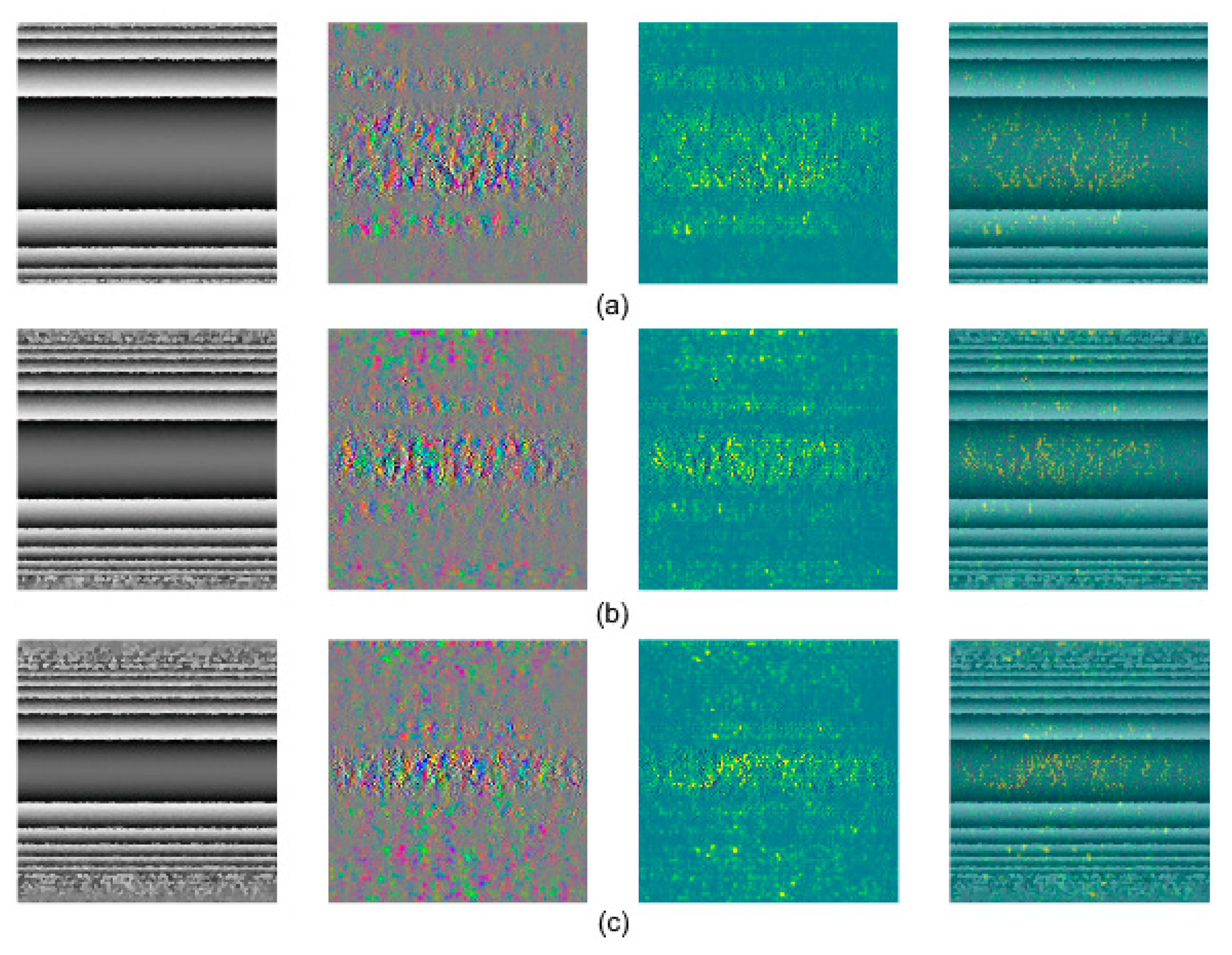
In addition, CNNs have a hierarchical organization in layers, which increases their processing capacity. A CNN has the ability to learn low and high levels of features, and the learned features are used to categorize the input image. A useful tool to understand how neural networks categorize the input images is a saliency map. Saliency maps analyze the learned features and offer a visualization of what the CNN uses to categorize. Saliency maps in computer vision can give indications of the image regions that have more impact on the final decision of the CNN. A gradient across the RGB output channel appears because the CNN works using three different filters, one for each RGB color. Then, the backpropagation step used by the CNN gives classification clues when it calculates the max gradient of the input image. In a saliency map, the dots in the max gradients are not noise, they indicate the pixels in the image that contribute to the output classification. The higher dot density in the phase difference maps is the central region, which strongly contributes to the CNN image classification.
Figure 6 shows some saliency maps randomly taken from this research. The saliency maps show that the CNN model is focused in the image lines due to the phase differences, and not on the noise generated by the high spatial frequencies.
2.4. Training Process
A total of 7200 images of six different classes were recorded. To create the train images dataset (1000 images per class), 6000 images were randomly taken. The remaining 1200 images were used to build the validation dataset (200 images per class). In addition, 1000 new images were recorded with intermediate concentration samples, which were used to prove the proposed method, and they were not used to train the CNN. The intermediate concentration samples were made with NaCl masses of: 0.375 g, 0.625 g, 0.875 g, 1.125 g, and 1.625 g.
The image size registered by the CCD camera was 1280 × 1024 pixels, however, the images were center cropped at 224 × 224 pixels, according to the input layer of the CNN.
The training process was developed and implemented using Google Colaboratory, a free cloud service for machine learning education. It provides a virtual machine on a GPU (graphics processing unit) of a Nvidia Tesla K80 with 2496 CUDA cores. ResNeXt was extracted from PyTorch torchvision package. For the training of the CNN, the algorithm executed a total training of 100 epochs with the optimizer of stochastic gradient descent (SGD). The epoch number was selected by analyzing the loss of training according to previous executions of the training process. The network was trained with a momentum of 0.9, and a stochastic gradient descent. The batch size was 40. The hyperparameters used in the experiment are listed in
Table 3.
2.5. Performance Metrics of the Proposed Method
The performance metrics were carried out in two stages. The first stage evaluated the performance of the CNN as an image classifier, and the second stage evaluated the performance of the Regressor as a concentration estimator.
2.5.1. Performance Metrics of the CNN
The confusion matrix is a metric for the evaluation of the CNN as image classifier. A confusion matrix is defined by four terms, which are: true positive (TP, elements predicted as elements that belong to a particular class, and that belong to that class); true negative (TN, elements predicted as elements that do not belong to a particular class, and that do not belong to that class); false positive (FP, elements predicted as elements that belong to a particular class, and that do not belong to that class ); false negative (FN, elements predicted as elements that do not belong to a particular class, and that belong to that class).
The
accuracy is defined as the percentage of the total number of predictions that were correctly classified and is calculated as:
where
N is the total number of elements to be classified.
The
precision is the ability to predict an element according to the class it belongs to and is defined as:
The
recall is the ability of the classifier to label all the positive cases and is calculated as:
The
specificity is the ability of the classifier to label all the negative cases and is defined as:
The
F-Score determines the precision of our classifier and is calculated as:
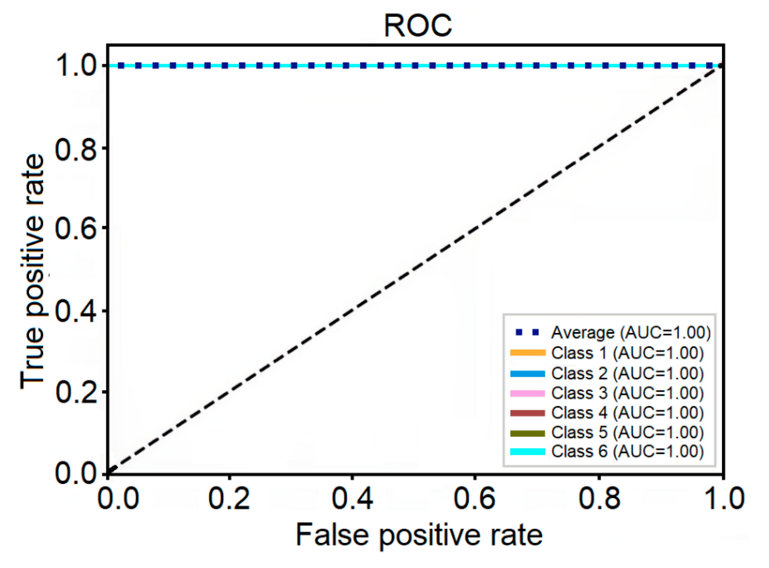
The receiver operating characteristic (ROC) is a graph of Recall versus Specificity. This graph characterizes the ability of a CNN to identify positive cases as positive, and negative cases as negative. Thereby, the area under the ROC curve (AUC) is the probability that a couple of positive and negative cases chosen at random are correctly classified.
2.5.2. Performance Metrics of the Regressor
The coefficient of determination (
) determines the quality of the model to replicate results. It is described as:
where
is the predicted value;
is the true value, and
is the average value of the
true data.
The mean absolute error (
MAE) is the mean of the difference between the true values and the predicted values. It is calculated as:
where n is the total number of data.
The mean square error (
MSE) is a statistical measure of the goodness of fit or reliability of the model according to the data. It is determined as:
3. Experimental Results and Discussion
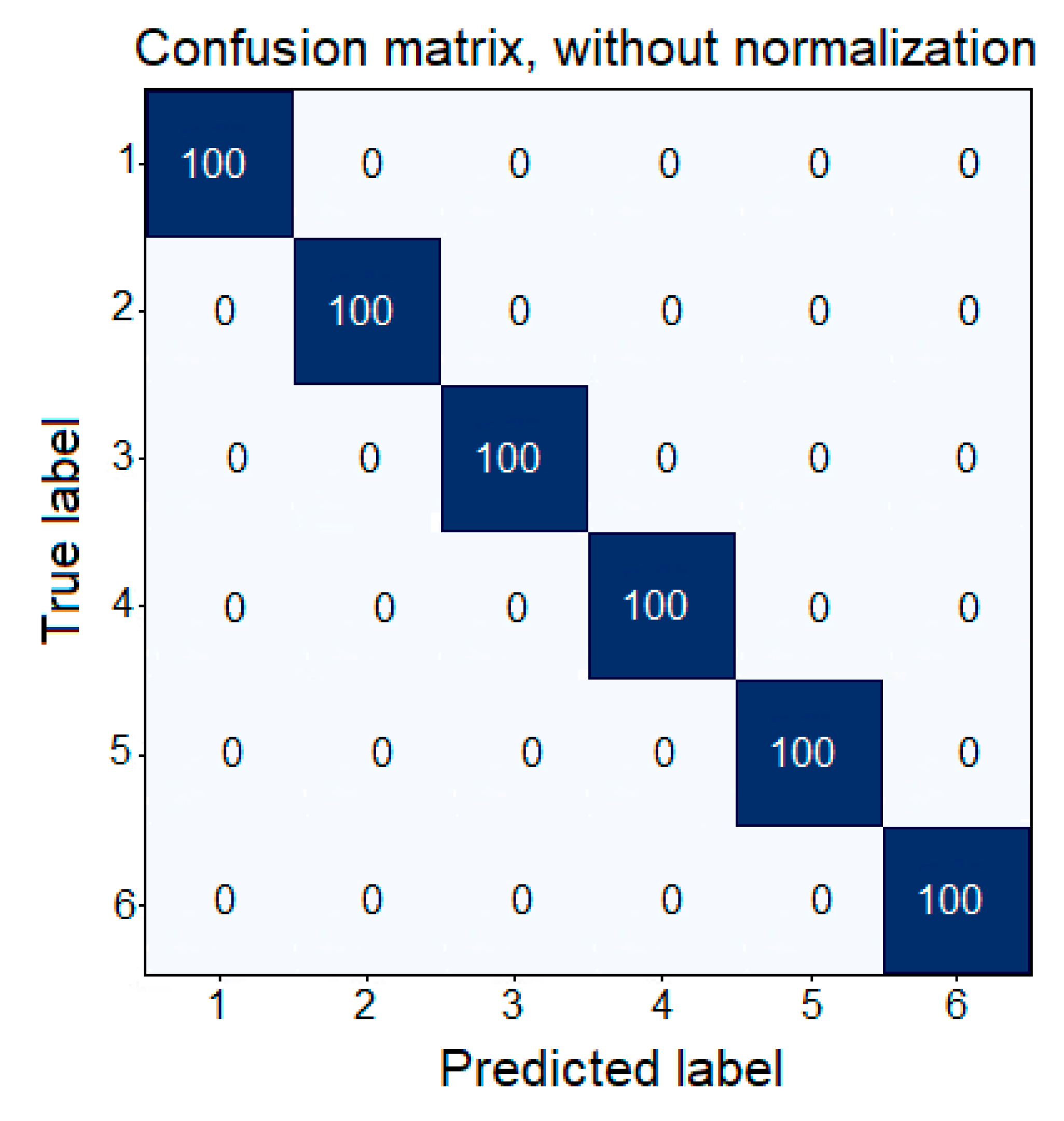
The performance metrics were evaluated with the validation dataset, which consisted of six classes with 200 images in each class. For the CNN evaluation as the image classifier, a perfect classification was reached in the confusion matrix. The confusion matrix reached is shown in
Figure 7. The confusion matrix obtained was a diagonal matrix, where the main diagonal elements reached the maximum classification percentage, i.e., the CNN correctly classified 100% of the images according with their classes.
Therefore, the performance metrics of the CNN as classifier reached the maximum score in accuracy, precision, recall, specificity, F-score, ROC, and AUC. The values of the performance metrics are shown in
Table 4, and the ROC in
Figure 8.
The performance of the Regressor as a phase difference estimator was also calculated, and the results obtained are shown in
Table 5. The Regressor presented a high coefficient of determination (
) of 0.9986, which indicates that it is a high-quality model. Also, the Regressor presented low values of MAE and MSE errors, which indicates that the model presented a good capacity to estimate. It is noted that the regressor reached a high performance, however, there are errors that guarantee that the CNN was not overfitted (the CNN did not memorize the images).
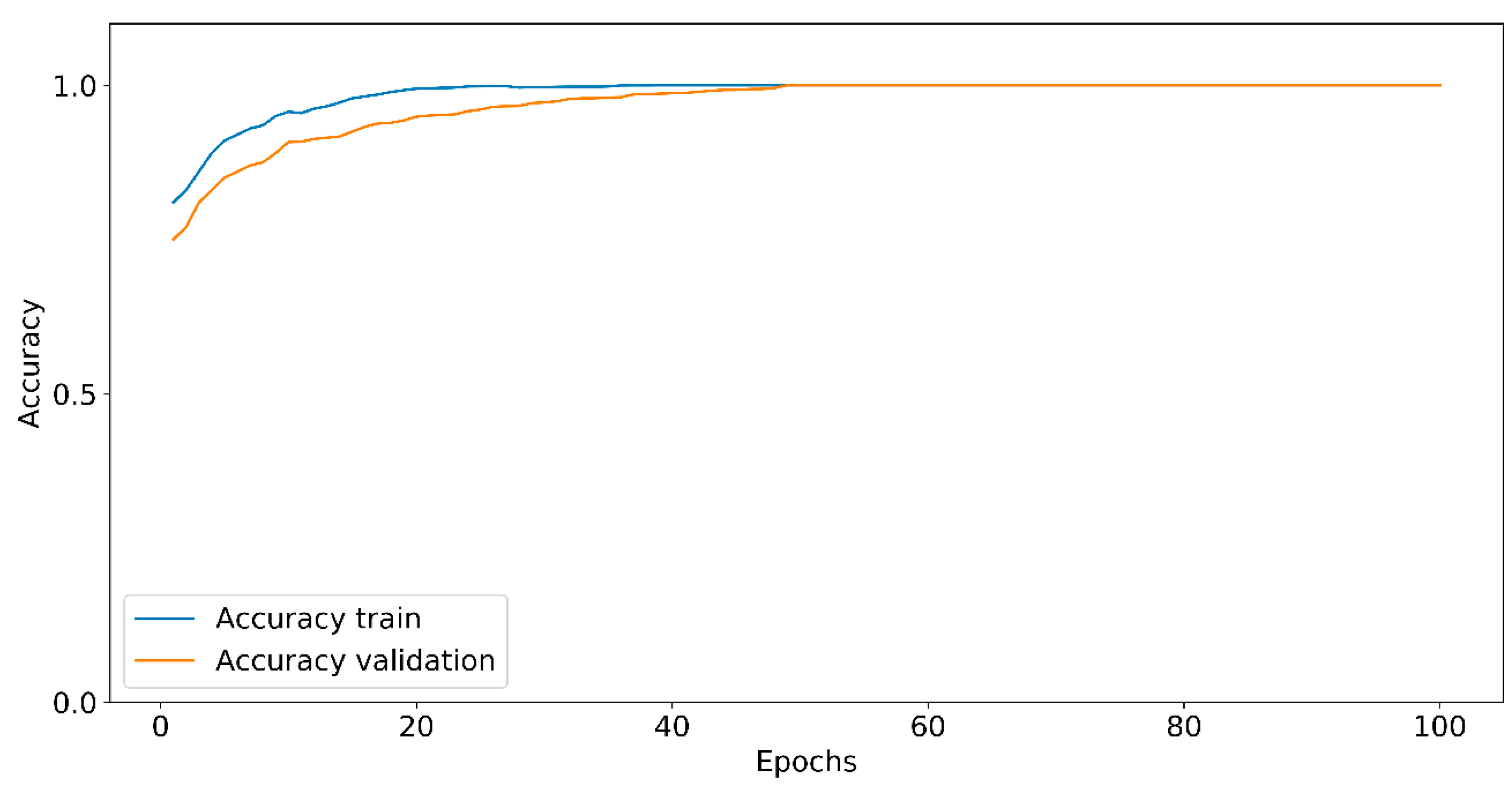
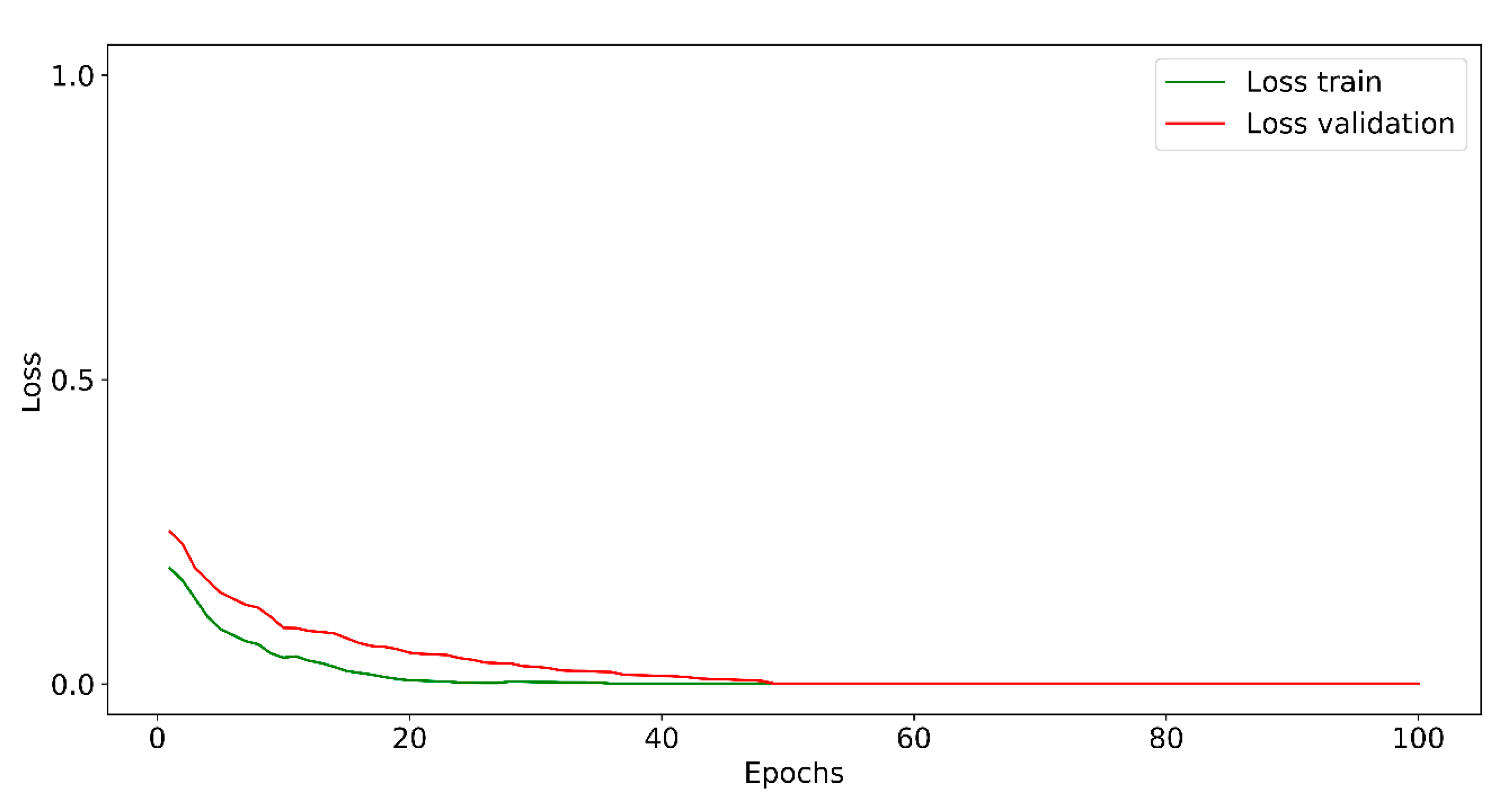
The training accuracy and training loss curves are shown in
Figure 9 and
Figure 10, respectively. The CNN obtained a high value of accuracy of 90% in its first epochs; however, the CNN accuracy presented fluctuations until the epoch 55 reached the maximum numerical score of accuracy.
The concentration values estimated by the proposed method with all the validation dataset are shown in
Table 6. The error relative between the true and predicted values, the standard deviation (STD), the mean absolute error (MAE), and the mean square error (MSE) per class are also listed in
Table 6.
According to the validation dataset, and the classes with which the CNN was trained, the proposed method presents a precision of ± 0.0147, and an accuracy of 0.0043%.
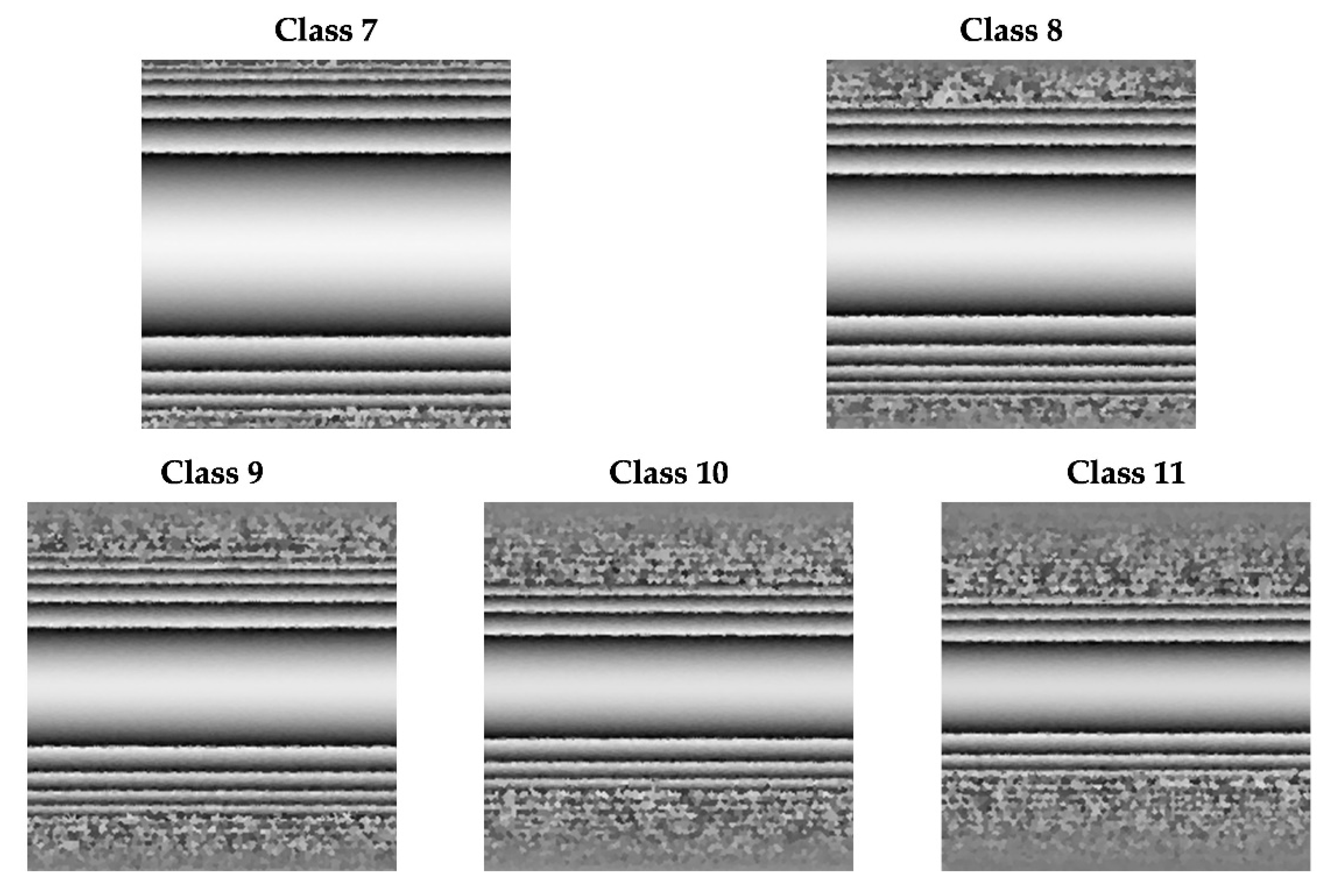
In addition, five new classes with different phases of difference were used to verify the proposed method. The difference phases estimated by the proposed method are shown in
Table 7. Also, the new holograms are shown in
Figure 11. These holograms were not used before in the training process.
It should be noted that the errors in
Table 6 are smaller than the values obtained with the conventional DHI method [
5]. However, in
Table 7 the errors are slightly higher; however, the precision can be improved if the image dataset is increased.
Therefore, the proposed method can calculate concentration ranges from 0.25 gL−1L to 1.5 gL−1, with a precision of ± 0.0645, and accuracy of 0.0731% based on data and classes that were not used to train the CNN.
4. Conclusions
In this paper, a new method to skip the phase unwrapping process in DHI based on CNNs is proposed. The CNN and the Regressor were used to estimate the concentrations of liquid samples in a cylindrical glass, using the images obtained with digital holographic interferometry. Using DHI to measure difference concentration values in liquid samples, large differences created phase map differences with high-frequency fringes, and the fringes appeared as noise. In addition, the liquid samples needed to be fragmented to create minor concentration liquid values, which created phase difference maps that could be correctly mapped by the sensor, and could be unwrapped with common methods.
Using a CNN, the concentration liquid samples were estimated using the phase map difference, and the unwrapping process was omitted. This method directly estimated the concentration values in liquid samples associated with difference phases, without the necessity of common phase unwrapping processes due to the CNN that was trained to quantify the phase wrapped images. In other words, the proposed method was able to estimate the concentration values from an input image based on the spatial distribution of the phase wrapped image without using the conventional phase equations. Although the differences among the image samples for each class could be obvious to the eye, their classification and quantification is not, and the CNN must be trained to estimate the sample concentrations that are different from those it was trained with.
In other words, our proposed method was able to estimate the concentration values for classes that were unknown based on the central region of the input image. The results showed a performance with high accuracy and precision. Once the CNN was trained and the Regressor was fitted, the proposed method was able to calculate the concentration values directly, with classes that were not used in the training process, as long as the values were in the operational range. As further work, a range extension could be performed, and a different form of the unwrapping phase based on CNNs could be analyzed.

 ,
, 


