An Analysis on the Effects of the Fuel Injection Rate Shape of the Diesel Spray Mixing Process Using a Numerical Simulation

Abstract

In diesel engines, fuel mixing is an important process in determining the combustion efficiency and emissions level. One of the measures used to achieve fuel mixing is controlling the nature and behavior of the fuel spray by shaping the injection rate. The mechanism underlying the behavior of the spray with varying injection rates before the start of combustion is not fully understood. Therefore, in this research, the fuel injection rate shape is investigated to assess the spraying and mixing behavior. Diesel sprays with different ambient temperatures and injection pressures are modeled using the CONVERGE-CFD software. The validation is performed based on experimental data from an Engine Combustion Network (ECN). The verified models are then used to analyze the characteristics of the diesel spray before and after the end-of-injection (EOI) with four fuel injection rate shapes, including a rectangular injection rate shape (RECT), a quick increase gradual decrease injection rate shape (QIGD), a gradual increase gradual decrease injection rate shape (GIGD), and a gradual increase quick decrease injection rate shape (GIQD). The spray vapor penetrations, liquid lengths, evaporation ratios, Sauter mean diameter (SMDs), distributions of turbulence kinetic energy, temperatures, and equivalence ratios were compared under different injection rate shapes. The results show that the QIGD injection rate shape can enhance mixing during injection, while the GIQD injection rate shape can achieve better mixing after the EOI.

1. Introduction

Diesel engines find widespread applications in many industries, including transportation, agriculture, and power generation, among others. Soot and NOx emissions, which are products of fuel combustion in these engines, pose a threat to the environment and the health of living organisms. Over the years, strict global regulations have been set to reduce the negative impact of such emissions. These stringent legislations require manufacturers to design cleaner and more efficient engines [1,2]. Many technologies, such as diesel particulate filters (DPFs) [1] and selective catalytic reduction (SCR) [3], have been developed to reduce emissions from diesel engines. In addition, controlling the combustion process (e.g., by using low-temperature combustion (LTC) [2], homogeneous charge compression ignition (HCCI) [4], reactivity-controlled compression ignition (RCCI) [5], and premixed charge compression ignition (PCCI)) have also attracted significant research interest [2]. Research on the fuel mixing process for preparing diesel combustion components in cylinders through effective injection rate adjustment is an important consideration. In this study, we only consider injection rate adjustment in the fuel injection system without changing the air intake and other contexts of the system; thus, this study does not modify the existing injection system too greatly. This is due to the significant influence of the air–fuel mixing process on combustion efficiency and exhaust emissions in diesel engines.

The latest developments in fuel injection strategy efficiency tend to focus on the injection rate to increase fuel mixing efficiency and reduce emissions. Notably, the combustion time will be shorter for cases with high initial injection rates. Generally, a high initial injection rate will result in better atomization and air entrainment. The duration of combustion decreases as the mixture of air and fuel improves, meaning that combustion occurs faster. Conversely, under a low initial injection rate, the initial atomization of the fuel and premixing are not good. The slow initial injection fuel droplets will combine with faster fuel droplets, which will result in a larger droplet size that yields a poor spray breakup. The combustion period will then be longer as more time is required to inject the fuel to atomize and evaporate it for combustion. In the past, researchers were interested in investigating the injection rates to improve fuel injection strategies. Juneja et al. [6] noted that increasing the injection rate after a previous injection is sufficient to increase the collision frequency and formation of large droplets, resulting in high momentum and greater penetration. Liu et al. [7] found that a higher peak injection rate yielded a higher spray tip penetration, peak entrainment rate, and entrainment rate after the end of injection (EOI). In addition, Arsie et al. [8] suggested that the start of injection is the main parameter that affects the impingement phenomenon, whereas Kun Lin Tay et al. [9] found that the start of combustion for each rate shape is different, although the injection duration and start of injection are same due to the start of pressure rise in each case. The peak in-cylinder pressures are higher when the start of combustion is advanced due to the injection rate shaping. The combustion duration will be shorter with a higher initial injection velocity. Apart from that, the results from numerical study on the effects of boot injection rate shapes by co-workers of Balaji Mohan and Kun Lin Tay [10,11,12], showed that NOx decreased but large soot particles occur due to low injection velocity and narrow soot distribution when the main injection velocity is higher [11]. Dezhi Zhou et al. [12] found that higher boot injection velocity and shorter boot injection duration resulted in shorter ignition delay and more fuel burning at the premixed combustion stage. This suggests that a higher injection pressure will often lead to a better spraying process, that this is one of the most effective ways to meet the efficiency requirements, and that this process has a potential benefit in diesel engine performance [13,14,15]. Agarwal et al. [16] found that increasing the injection pressure reduces the number and mass of particles and increases the diesel spray velocity, which improves the atomization and evaporation process. In addition, Shuai et al. [17] applied a numerical simulation to examine the effects of injection time and injection rate shape on the performance and exhaust emissions of compression ignition engines. The authors found that CO, UHC, and soot emissions can be reduced by using rectangular-type and boot-type rate shapes instead of other types. Based on these previous studies, the injection rate is clearly an important parameter that requires more attention. Injection rate parameters, such as injection velocity, injection mass quantity, and injection duration, have a significant influence on the fuel mixing and combustion process [18]. Many of these investigations considered how the diesel spray mixing process behavior can increase mixing efficiency by studying the effect of the injection rate shape. Attempts to increase fuel mixing efficiency by determining the injection rate shape remain unsatisfactory. Although there have been extensive studies in the past on the influence of injection rates, most of these studies were interested in investigating the influence of injection rates on combustion efficiency and engine emissions [9,10,11,12,17]. Few studies have investigated the influence of injection rates on spray mixing behavior.

Based on our previous study [19], we examined the spray mixing characteristics under different injection rate shapes using a modified one-dimensional spray model. This one-dimensional spray model can analyze the spray penetration, entrainment rate, and velocity over a cross-sectional area, as well as the equivalence ratio distributed along with the spray’s axial distance. This model does not consider breakup and evaporation. Instead, it reveals general information on both the liquid and the vapor. The fuel and air are assumed to be immediately mixed uniformly, so turbulent mixing cannot be analyzed in detail. A 3D-CFD model is better for researching a spray that includes two-phase flow characteristics.

Creating a spray model using CFD has become an effective way to study diesel spray to analyze the mechanism of fuel–air mixing and atomization. The results of many previous studies on creating a spray model using CFD show that the various parameters of fuel injection can be efficiently monitored and predicted [20,21,22]. Nevertheless, there are few studies on the injection rate shape’s effects on spray mixing. Unlike a quasi-steady-state spray, it is difficult to obtain clear spray images that include liquid and vapor information under varying injection rates, so there is a lack of experimental data to validate the 3D-CFD spray model with varying injection rates. Consequently, most numerical studies focus on the effects of injection rates on combustion processes and do not offer an in-depth understanding of the spray behaviors under different injection rates.

The objective of the current study is to analyze the effect of different injection rate shapes on the diesel mixing process using a numerical modeling method. In this work, the “CONVERGE” CFD code was adopted for a constant-volume combustion chamber with a single hole injector, particularly to study the spray breakup and spray mixing behavior. Validation of the model results involved a comparison of the spray shape and spray penetration with the experimental data from previous researchers of the Sandia National Laboratory, taken from the ECN website [23]. We found that the modified CFD spray model can predict spray behavior. Four injection rate shapes were used to analyze the effects of injection rate shapes on diesel spray mixing behavior to understand the mixing process in-depth, including the microscopic spray characteristics, evaporation process, and mixture properties. The results of this study are expected to provide useful insights for developing an effective fuel injection rate design for future diesel engines.

2. Numerical Modeling

In this study, numerical simulations were implemented using CONVERGE Version 2.2 [24], which was used to create constant volume models and set the turbulence model, spray model, and sub-model, as shown in

Table 1. Modeling and Numerical Parameters.

Modeling Tool	CONVERGE
Spray models
Drop evaporation model	Frossling model
Collision model	No Time Counter model (NTC) collision
Collision outcome	O’Rourke collision outcomes
Drop drag model	Dynamic drop drags
Breakup	KH-RT model
Turbulence model	RANS, RNG k-ε
Grid control
Base grid size	16 mm
Finest grid size	0.25 mm

. This model was created to predict the diesel spray performance by simulating the spray shape and the spray penetration distance in both a liquid and a vapor state, as well as the mixing behavior. The shape of the model is defined as a constant volume combustion chamber with a diameter of 105 mm and a length of 105 mm to reduce the grid number and increase computational efficiency, with input from the case study boundary conditions under the experimental conditions [23]. The injector was placed at the top center of the cylinder, as shown in Figure 1. The spray was designed using the Spray A condition (detailed information is shown in the ECN [23]). The C₁₂H₂₆ reaction mechanism was used as a diesel fuel agent like the experimental considerations since the current model estimation of the trends and evolution of vapor penetration are independent of the fuel type [25].

The grid size has a large influence on the penetration distance [26]. When the grid size is too small, a long simulation time will be required. In this study set up, a fixed grid embedded with a minimum grid size for the spray flow field is shown in Equation (1) [24], where the “Size of cells in scaled grid” represents the sizes of the cells in the scaled grid in each axial “Size of cells in base grid” indicates the sizes of the cells in the base grid setting of each axial, and “amr_embed_vel_scale” is the level of embedding. In this study, CONVERGE can easily change the overall grid resolution prior to executing a simulation to assess grid sensitivity, which is useful for reducing the working time for constant stimulation. For simulations in areas or periods that are not of great importance, a rough grid can be used and then adjusted to consider only the important periods by setting the level of embedding for each section to obtain results that are accurate and not unnecessarily time intensive for calculations:

$$Sizeofcellsinscaledgrid=Sizeofcellsinbasegrid\ast 2^{-amr\_embed\_vel\_scale}.$$

(1)

The computational fluid dynamics simulation of the in-cylinder process has many modifications in the spray modeling. The interaction of spray turbulence modeling has an important influence on the spray penetration and mixture formation prediction, which emerges at the end of the entire combustion process. A recent literature review on fuel spray modeling showed that the use of RANS guidelines is of fundamental importance to ensure sufficient performance of the spray mixing and combustion processes. In this study, we used the RANS method to describe the spray development process. The RANS model was used in conjunction with the RNG k-ε turbulence model to determine the effects of smaller movements. A drop evaporation model base on the Frossling model was also used. The liquid penetration length is defined as the maximum distance from the axial position with 99% injected fuel mass at the injection location, while the vapor penetration length is defined as the distance from the farthest location with a 0.01% fuel mass fraction to the nozzle exit. For a fast and accurate collision calculation response, the NTC model with an O’Rourke outcome was used in this study. To increase the efficiency of our droplet collision calculations, we used a dynamically simulated gas technique for spraying. For this technique to work effectively, it must be able to handle a common case, where the number of droplets in each particle varies. The configuration can work effectively with general cases under different conditions.

For the spray breakup model in this study, the Kelvin–Helmholtz instability (KH) and Rayleigh–Taylor instability (RT) models were used. The KH model size constant is defined as proposed by Reitz [27]. The wave breakup formulation was used to model the liquid breakup process. The wavelength (Λ_KH) and the breakup size constant (B₀) determined the child droplet sizes. The drop radius equation is calculated as follows:

$${\mathrm{r}}_{\mathrm{K}\mathrm{H}}={\mathrm{B}}_0{\Lambda }_{\mathrm{K}\mathrm{H}}.$$

(2)

By requiring that B₀ equal 0.61 for the droplet breakup regime that has the characteristics of 25 < We < 50, under a higher injection velocity, the B₀ will be in accordance with the applications offered by Hwang et al. [28]. The KH model velocity constant was determined to be 0.188, which is the basic value commonly used by researchers. During the breakup, the parent droplet parcel radius (r) is continuously reduced until it reaches a stable droplet radius (r_KH) according to the following equation:

$$\frac{\mathrm{d}\mathrm{r}}{\mathrm{d}\mathrm{t}}=\frac{\mathrm{r}-{\mathrm{r}}_{\mathrm{K}\mathrm{H}}}{{\mathsf{\tau }}_{\mathrm{K}\mathrm{H}}}, {\mathrm{r}}_{\mathrm{K}\mathrm{H}}\le \mathrm{r}$$

(3)

where τ_KH is the breakup time, given by:

$${\mathsf{\tau }}_{\mathrm{K}\mathrm{H}}=\frac{3.276{\mathrm{B}}_1\mathrm{r}}{{\Lambda }_{\mathrm{K}\mathrm{H}}{\mathsf{\Omega }}_{\mathrm{K}\mathrm{H}}}$$

(4)

where Ω_KH is the KH wave with the maximum growth rate. The KH model breakup time constant (B₁) determines the primary breakup time. In this study, B₁ equals 21, which is more accurate than the recommended value (recommended value equals 7) in other references. The RT breakup length equation is given by:

$${\mathrm{L}}_{\mathrm{b}}={\mathrm{C}}_{\mathrm{b}\mathrm{l}}\sqrt{\frac{{\mathsf{\rho }}_{\mathrm{l}}}{{\mathsf{\rho }}_{\mathrm{g}}}}{\mathrm{d}}_0$$

(5)

where C_bl is the RT model breakup length constant, ρ_l is the fuel density, ρ_g is the ambient gas density, and d₀ is the orifice diameter. The RT model breakup length constant (C_bl) generally equals 1.0.

It is necessary to switch the liquid breakup parameter from the KH model to the RT model. Using this approach, the breakup time can be determined by the RT model breakup time constant (C_τ). The value of C_τ should be less to reduce the breakup delay, as shown in the RT breakup time equation below:

$${\mathsf{\tau }}_{\mathrm{R}\mathrm{T}}={\mathrm{C}}_{\mathsf{\tau }}\frac{1}{{\mathsf{\Omega }}_{\mathrm{R}\mathrm{T}}}$$

(6)

where Ω_RT is the RT wave with the maximum growth rate. The RT model size constant (C_RT) used to determine the scaled wavelengths and the radius of the RT breakup with a higher value increases the predicted RT breakup radius size:

$$\mathrm{r}=\mathsf{\pi }\frac{{\mathrm{C}}_{\mathrm{R}\mathrm{T}}}{{\mathrm{K}}_{\mathrm{R}\mathrm{T}}}$$

(7)

where K_RT is the wavenumber. In this study, C_RT equals 0.1, in which the parent radius decreases continuously until it reaches the constant value in Equation (3), as in the KH model. The setting of the spray breakup model provides an additional configuration for the breakup model constants. Notably, different breakup model constants are used depending on the test conditions and the numerical calculation tools.

The spray dispersion angle is another important input variable. The spray distribution angle defines the fluctuation of air in the injected fuel due to the impulse exchange between gases and liquids. The spray distribution angle will change under different injection intervals (start of injection, the transient regime, the stable regime, and the EOI) due to changes in the nozzle sac flow, momentum, and the interactions between air and the fuel. The actual spray distribution angle detected by each method is different and cannot be compared. The differences in the spray distribution angles measured in the far-field show a higher angle variance than when measuring the angles using the near field method. Generally, the spray distribution angle can be represented in two ways: the spray angle and the spray cone angle. This study analyzed the shapes of different injection rates that have different injection pressures, making the spray distribution angle a very important variable because it is influenced by pressure. Here, the spray distribution angle is measured by taking an image of the cut-plane from the direction of the spray by specifying two lines to determine the area of the spray and then measuring the distribution angle. The spray angle is measured from the nozzle outlet to the spray penetration distance/2 and the spray cone angle is measured from the nozzle outlet to the spray penetration distance equal to the 100×hole diameter. The spray cone angles were used in this study as the input in the spray model to analyze the spray behavior. In this study, the spray cone angles changes depend on the operating conditions of the difference in rail pressure. The spray cone angle will increase noticeably when the injection pressure is higher because the pressure of the fuel mixture inside the nozzle increases and the distribution is higher. The relationship between spray cone angle and injection pressure is discussed in the fourth section.

3. Model Validation

In this section, the numerical models above were studied using a real experiment. Two different sets of operating conditions were used for predicting the spray behavior, including the spray shape, the spray penetration, and the equivalence ratio. The first set involves the model calibration using an evaporation process under experimental conditions at different ambient temperatures. The second set involves the model being calibrated at different rail pressures using the experimental conditions of the Sandia National Laboratory in the ECN [23]. The ambient density, steady flow discharge coefficient, and nozzle hole diameter are the same in all conditions (22.8 kg/m³, 0.89 mm, and 0.084 mm, respectively) and with the other conditions different, as shown in

Table 2. The Operating Conditions of the Test Cases.

Case No.	Ambient Composition	Ambient Temperature [K]	Ambient Pressure [MPa]	Fuel Temperature [K]	Injection Duration [ms]	Injection Mass [mg]	Rail Pressure [MPa]
1	N2 = 100.0	440	2.93	363	1.54	3.46	150
2	O2 = 0.00; N2 = 89.71; CO2 = 6.52; H2O = 3.77	900	6.05	373	1.54	3.46	150
3	O2 = 0.00; N2 = 89.71; CO2 = 6.52; H2O = 3.77	900	6.07	373	5.2	9.30	100
4	O2 = 0.00; N2 = 89.71; CO2 = 6.52; H2O = 3.77	900	6.07	373	5.65	6.90	50

.

The injection rate of the test conditions conducted by the Sandia National Laboratory in the ECN was determined by CMT, in which the injection mass flow rate of the Spray A condition was created using the “Virtual Injection Rate Generator” model on the ECN website. The virtual injection rate generator model considers the expected hydraulic fluctuations, including the injector opening times, the pressure, the nozzle diameter, and the discharge coefficient.

3.1. Ambient Temperature Effects

In this section, the low and high ambient temperature conditions are used for model calibration. To demonstrate the predictive efficiency of the model, the spray behavior under different ambient temperatures, as well as at different ambient pressures (case No. 1 and 2 in Table 2) is used as a case study.

A comparison of the fuel spray injection in the cylinder at different ambient temperatures and ambient pressures shows the influence of evaporation and spray fuel diffusion. Figure 2 and Figure 3 present a comparison of the spray shape and equivalence ratio between the experimental and simulation results for cases No. 1 and 2. The gray background images show the experimental data obtained from high-speed videos using the Schlieren video technique to represent the vapor and liquid for case No. 1. For case No. 2, the experimental data image obtained from the high-speed video using the Schlieren video technique shows vapor and liquid regions, which are stored as MATLAB binary files. The white background images show the simulation result, in which the gradient color region represents the equivalence ratio data. The value of the equivalence ratio is represented by the gradient color bar in the right corner. The black particles are liquid fuel data from the simulation, which the cut-plane from the direction of the spray then rotates 90° to the left. Figure 2 and Figure 3 illustrate the shape of the variance by using Re-Normalization Group Theory to determine the small movement effects, while the KH-ACT model calculation captures the impact of cavitation and turbulence on the primary cracks in addition to aerodynamic separation. The calculation results show a smoother distribution for the spray shape boundary simulation than for the experimental data due to the turbulence model’s limitations in conjunction with the RNG k-ε turbulence model, where the RNG k-ε turbulence model is used for determining the smaller movements effects. Nonetheless, the simulation results are satisfactory, as these results indicate the effective grid resolution for this simulation. Each comparison image shows the exact thickness of the fuel mass distributed throughout and is consistent with the experimental data. The method of image analysis obtained from this model is sufficient for the study of spray behavior.

The comparison results (Figure 4 and Figure 6) show the spray penetration and spray distribution angle. Black and red represent the results under ambient temperatures of 440 and 900 K, respectively, while dots and solid lines represent the experimental and simulation results, respectively.

The results of vapor penetration are shown in the top graphs of Figure 4 and Figure 5, while the middle and bottom graphs show the liquid penetration and injection rates, respectively.

Figure 4 shows the simulation results that are compatible with the experimental results both during injection and after the EOI. The initial injection is important to consider, as it provides the momentum to change the conditions in the combustion chamber caused by the onset of fuel injection, thereby increasing the injection rate, temperature, and pressure. As shown in Figure 5, the initial spray penetration (0.0–0.3 ms) reveals that both cases cannot properly capture the initial ramp for both vapor and liquid penetration. Due to the very short time error of the simulation results (less than 0.1 ms), the injection rate input data from the virtual injection rate generator may not be as accurate as those of the actual injection rate.

Figure 6 shows a comparison of the spray angle (left graph) and the spray cone angle (right graph) with varying ambient temperatures. The measurement results from experimental data show that the ambient temperature influences the spray angle but not on the spray cone angle. The trend of the measurement results of the spray cone angle is the same for both cases, which means that the spray cone angle is independent of the ambient temperature and ambient pressure. In addition, the simulated spray cone angle results show the same trend as the measured experimental results. These results show that the constructed model effectively predicted spray behavior under varying conditions of ambient temperature and ambient pressure.

3.2. Rail Pressure Effects

To ensure that the effects of rail pressure changes are captured by the model when predicting the spray’s behavior between the start of the injection (lamping up) and the end of the injection (lamping down), the experimental conditions from previous ECN work under operating conditions No. 2, 3, and 4 (as described in Table 2) are studied in this section.

Figure 7 and Figure 8 show a comparison of the spray shape and equivalence ratio between the simulation results and the experimental data of the rail pressure under 100 MPa and 50 MPa conditions, respectively. The gray background images show the experimental data obtained from high-speed videos using the Schlieren video technique. The white background images show the simulation results. The gradient color region represents the equivalence ratio data, with values shown on the gradient color bar in the right corner.

The black particles are the liquid fuel data from the simulation, which the cut-plane from the direction of the spray then rotates 90° to the left (which is similar to the display in case No. 2, as mentioned in the previous section (Figure 3)). From these comparisons, the results of the simulation show a better prediction under high rail pressure conditions (150 MPa and 100 MPa) than under a low rail pressure condition (50 MPa).

The results of the spray penetration and spray distribution angle (Figure 9 and Figure 10) shown in the red, blue, and yellow colors indicate the results for rail pressures of 150, 100, and 50 MPa, respectively. The dots and solid lines represent the experimental and simulation results, respectively. The results of vapor penetration are shown in the top graphs of Figure 9 and Figure 10, while the middle and bottom graphs show the liquid penetration and injection rates, respectively.

Figure 9 shows that the model predictions for the penetration length under high rail pressure conditions are longer than those under low rail pressure conditions, which is consistent with the experimental data. Figure 10 shows the initial spray penetration (0.0–0.3 ms); even under the rail pressure conditions in all three cases, these data cannot properly capture the initial ramp for both vapor and liquid penetration. The simulation results show a trend that is consistent with the experimental data. The spray model and other sub-parameters make this model more effective in its predictions, which is consistent with experimental data.

The rail pressure directly affected the air fluctuation in the injected fuel due to the impulse exchange between the gas and the liquid. The spraying behavior under high rail pressure caused the cavitation flow to efficiently accelerate at the nozzle exit. The high rail pressure cavity also increased the spray distribution angle [22]. Figure 11 shows a comparison of the spray angles (left graph) and the spray cone angles (right graph) for different rail pressures, in which the spray distribution angle is measured by the same technique described in the previous section. It was found that the size of the spray angle is not constant, but the spray cone angle from the measured simulation results shows a similar trend to the experiment. This confirms that the spray cone angle size setup in this model is correct and can thus predict the experimental data with acceptable accuracy.

The above results show that different rail pressure conditions affect the spray’s infiltration behavior. The generated model shows good predictive performance when there is a change in the working conditions. These results demonstrate that this model can predict the spray’s permeability and injection characteristics at an acceptable level. This model will be used for spray behavior predictions to analyze the behavior and mixing processes of diesel spray with different injection rate shapes in the next section.

4. Effect of the Injection Rate Shape

The injection rate shape is an important factor that affects the spray formation. After leaving the injector, the fuel spray atomizes into droplets, vaporizes, and mixes with the air. In this work, models with different injection rate shapes are analyzed for their spray and fuel mixing behavior using the basic conditions from the previous work on ECN case No. 2, as shown in Table 2. The four injection rate shapes shown in Figure 12 were selected for this study. The rectangular injection rate (RECT) shape is the constant injection rate and is a commonly used injection rate shape. The other three shapes consist of the Quick Increase Gradual Decrease injection rate (QIGD), the Gradual Increase Gradual Decrease injection rate (GIGD), and the Gradual Increase Quick Decrease injection rate (GIQD). These shapes were designed to examine the effects of an increase and a decrease of the injection rate over a short injection duration to study the influence of spray and combustion behavioral control factors based on previously reviewed research. The above factors include the peak injection rate, the initial injection rate, and the injection velocity of each injection period, which are useful for understanding the spray and fuel mixing behavior. The four injection rate shapes must have the same injection duration and fuel quantity to be used as a benchmark. The three shapes (QIDG, GIGD, and GIQD) had peak injection rates higher than the experimental conditions in case No. 2, which means that the rail pressure would be higher than 150 MPa. As shown in the simulation model, these injection rate shapes can create a peak rail pressure of approximately 600 MPa. A maximum rail pressure of 600 MPa is too high for current engine technology. In this study, the maximum rail pressure generated by the injection rate was determined from the study conditions according to the constant value of the injection duration with the same amount of fuel as used in the experimental data to ensure that the model calibrated from the experiment data would be accurate. The injection pressure can be increased by changing the injection rate of the fuel pump and adjusting the injector area. If the injection pressure is too high, the ignition delay period will be shorter. This may cause a homogeneous decrease in mixing and reduce the combustion efficiency. In practice, changing the injection rate and injector area is necessary to help reduce these effects.

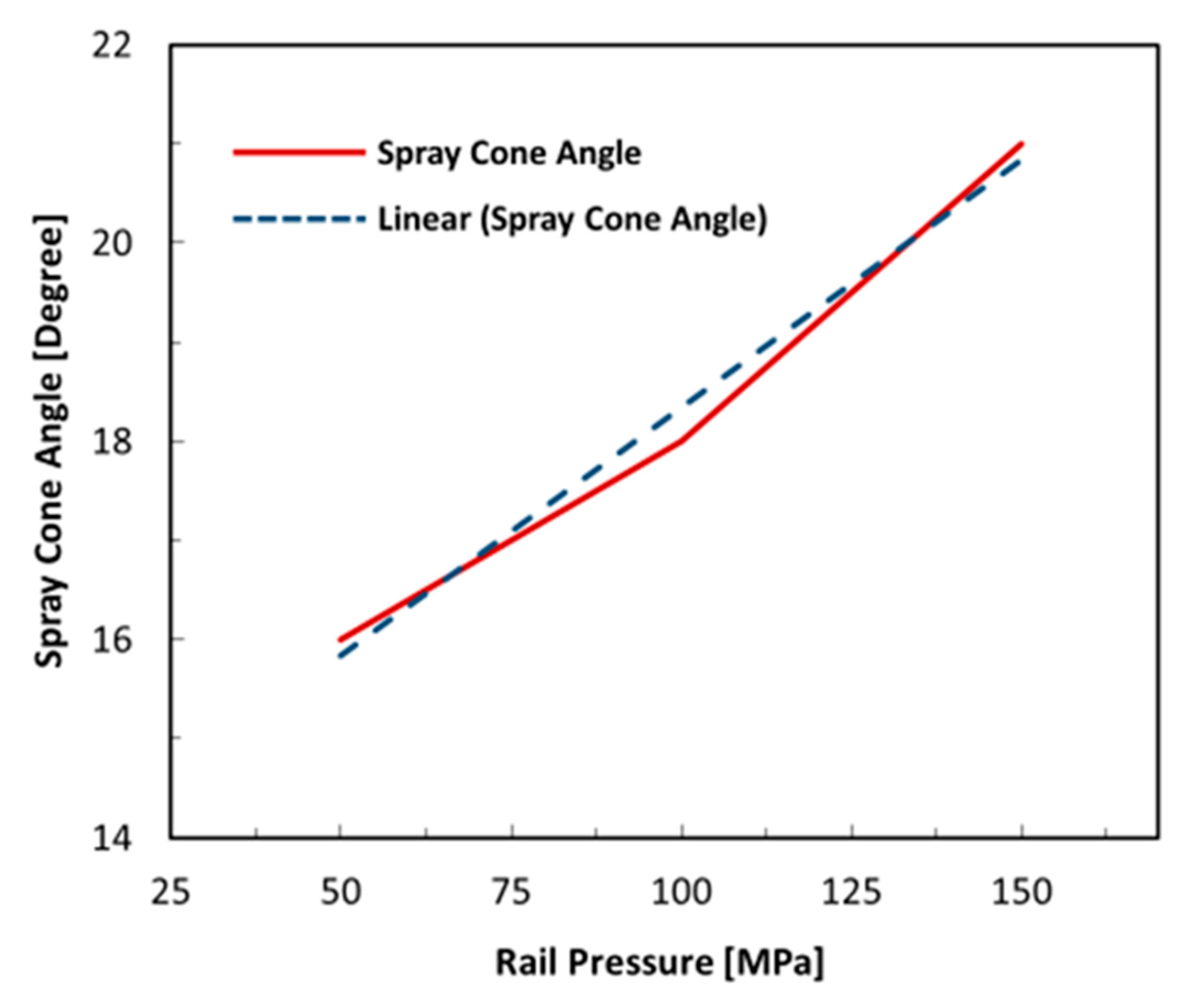
As a result that the newly created injection rate shape for this study is determined by a constant injection duration and fuel mass (including under ambient conditions, which are similar to those of the experimental data), under some conditions, this novel injection rate provides a peak injection rate that is higher than the injection rate of the experimental data used to calibrate the model. This means that higher injection rates will also result in higher rail pressure. Although this study explored the maximum rail pressure conditions up to 600 MPa, the results calibrated with the experimental data for rail pressure of 50, 100, and 150 MPa showed that the model can provide reliable simulation results, even under conditions where the pressure is different. In particular, the simulation results show that the study conditions at a maximum rail pressure of 150 MPa can provide better simulation results than under conditions of a lower maximum rail pressure. This means that the newly created model is effective for high rail pressure conditions. In addition, in this paper, all case studies (including the cases of maximum rail pressure conditions of 600 MPa) use ambient conditions. The injection timing and the fuel mass are the same as those of the experimental conditions at a rail pressure of 150 MPa because the simulation results for the calibration under rail pressure conditions of 150 MPa give good results for both quantity and volume. The prediction results for the spray shape are compatible with the photos from the experimental data; this shape reflects the accuracy of the distribution angle, penetration, and evaporation of the spray. The injection rate and injection pressure have a great influence on these physical characteristics. Therefore, the model created can predict the spray behavior very well, especially under high rail pressure conditions. Based on the study of the effects of different rail pressures, the spray shape data from the experiment demonstrate that the size of the spray cone angle is different under the same ambient conditions, as shown in Figure 13. Figure 13 shows the spray cone angle size obtained from the spray picture of the experiment data. The result indicates that the spray cone angle used as the input data in this study depends on the size of the maximum rail pressure. The model calibration demonstrated that using the spray cone angles obtained from the experimental spray images as inputs can provide good predictive results (consistent with the experimental data). Therefore, this study used the prediction equation (Equation (8)) to predict the size of the spray cone angle at different rail pressures:

$$Sray cone angle=0.05P_{rail}+13.333.$$

(8)

4.1. Microscopic Spray Characteristics

In spraying simulations, the turbulent distribution has a significant impact on the spray parameters. The spray penetration distance depends on the surrounding conditions, including the injection rate, the injection time, the injected mass quantity, and others. The injection rate design affects the spray penetration and spray distribution angle. This section presents the spray penetration distance consisting of liquid and vapor penetration both during the injection time (0–1.54 ms) and after the EOI, by comparing the results of different injection rate shapes and using these shapes to analyze their effects on the microscopic spray characteristics.

Figure 14 shows the simulation results of the spray penetrations. The black, red, blue, and yellow lines represent the simulation results for the RECT, QIGD, GIGD, and GIQD injection rates, respectively. The results of vapor penetration are shown in the top graph, while the middle and bottom graphs show the liquid penetration and injection mass flow rates, respectively. Figure 14 (top graph) shows the vapor penetration for the four injection rates with different shapes. The QIGD injection rates show the longest vapor penetration (approximately 25 mm), with an injection rate of around 4.5 mg/ms. Vapor penetration lengths with the same peak injection rates will ultimately lead to the same vapor penetrations. This occurs because, during injection, vapor penetration increases with the injection acceleration rate. After the EOI, the vapor penetration distance increases along with the injection rate at the EOI, when the spray penetration distance is affected by the momentum flux ratio. For the GIQD injection rate shape after the EOI, the vapor penetration continues to increase continuously, and a high injection rate results in rapid fuel movement, while the vapor penetration of the QIGD injection rate shape decreases continuously because of the injection rate at the EOI. Figure 14 (middle graph) shows the liquid spray penetration, for which the different injection rates also have a significant impact on liquid penetration. The QIGD injection rate provides the longest initial liquid penetration due to having the highest injection rate, while the GIQD injection rate shows the opposite. Liquid spray penetration increases relative to the injection rate shape and terminates at the end of injection. The liquid spray penetration results show the same trend as the injection rate for all cases. Since the greatest penetration distance is primarily affected by the momentum flux ratio, the liquid penetration distance will increase when the injection rate increases and decrease when the injection rate decreases. This is due to slowdown in the movement of the liquid fuel.

In addition, because the spray penetration is a phenomenon that occurs in conjunction with the spray distribution, the spray distribution angle is an important parameter that affects the spray mixing process and is important for the analysis of spray performance. Therefore, the spray distribution angle was investigated by measuring the distribution angle via the spray shape obtained from the simulation. Figure 15 shows the spray distribution angles from the simulation results, where the black, red, blue, and yellow dots represent the measurement results of the RECT, QIGD, GIGD, and GIQD injection rates, respectively. As shown in the Figure 14, comparisons were made between the spray angle (left graph) and spray cone angle (right graph) under different injection rate shapes. Similar techniques to those in the previous section were used to measure the spray distribution angles.

The same spray cone angle measurement results are shown in Figure 15 (right graph) for the same peak injection rate (same peak rail pressure) with different injection rate shapes; the results agree with those in the previous section. The shape with a peak rail pressure of 600 MPa and a spray cone angle of 43° will have spray cone angle larger than approximately twice that of the peak rail pressure of 150 MPa (21°).

Figure 15 (left graph) shows a difference in the spray angle event under the same peak rail pressure. The spray angle increases when the acceleration of the injection rate increases. It can be observed that the QIGD injection rate is significantly small but features a continuous decrease in the spray angle compared to the other injection rates. On the other hand, the GIQD injection rate recorded the largest spray angle at the beginning, followed by a slight decrease, and then remained constant (compared to the other injection rates). This phenomenon demonstrates that the increased injection acceleration rate has a significant effect on the fuel distribution ability, which directly affects the spray angle size. The spray angle is higher when the injection rate is higher because the injection rate can increase the rail pressure, thereby resulting in a higher particle force that can cause a higher penetration force leading to better distribution. The spray angle is an important parameter that helps us understand the global characteristics of the spray. The spray angle and quantity evaluation provide useful information about the airflow in the spray [29,30,31], where the spray angle is an indicator of gas. In general, the greater the spray angle, the higher the increase in gas entrainment, resulting in improved mixing [32]. Another interesting observation is the effect of the injection rate shapes on spray penetration. The simulation results reveal longer vapor penetration at a higher peak injection rate due to the efficient spray distribution, while the lower peak injection rate yielded poor vapor penetration because the low injection rate resulted in poor spray distribution and spray penetration performance. A spray tip that penetrates too long will result in wet combustion chamber walls, causing excessive soot formation and a waste of fuel. On the other hand, if the penetration time is too short, the mixing efficiency and optimum combustion will be compromised. In addition, the simulation results show that the QIGD injection rate with a high initial fuel injection rate quickly causes the initial penetration. This suggests that the injected fuel is very well atomized and has a significant effect on the onset speed of the combustion phenomenon. In the case of the GIQD injection rate, a very low initial injection rate may result in poor fuel atomization and cause an increase in the ignition delay. The evaporation process and mixing behavior will be discussed further in the next section.

4.2. Evaporation Process

We next studied the evaporation process influenced by the fuel injection rate by considering the distribution of droplet sizes. This section presents the simulation results of the evaporation ratio under different injection rate shape conditions, as shown in Figure 16. The simulation results show that different injection rate shapes result in different evaporation ratios. The results of the evaporation ratios are shown in the top graph, and the injection mass flow rates are shown in the bottom graph, where the black, red, blue, and yellow lines represent the simulation results of the RECT, QIGD, GIGD, and GIQD injection rates, respectively. Figure 16 shows that the RECT and the QIGD injection rate shapes undergo more rapid evaporation than the other injection rate shapes. As demonstrated by the RECT and the QIGD injection rate shapes, the evaporation ratio increases to nearly one before approximately 0.01 ms. For the GIGD and GIQD injection rates, the evaporation ratio increases to nearly one at approximately 0.1 ms. These results are due to both injection rate shapes having a quickly increasing initial injection rate, thereby resulting in high rail pressure, which can improve the evaporation rate because higher rail pressure results in a high shear of the fuel particles, which can change the fuel state from liquid to gas very quickly with higher mass flow rates, as well as accelerate the fuel evaporation process.

To better understand the spray breakup characteristics, the SMD is an important parameter that should be considered to reflect the spray performance. The size of the SMD is related to droplet breakup, in which a smaller SMD result in better droplet breakup. Due to the lack of experimental data to calibrate the simulated SMD results, only the relationship between the SMD and injection rate have been considered. Figure 17 shows the relationships of the SMD values for different injection rate shapes, where the black, red, blue, and yellow lines represent the simulation results of the RECT, QIGD, GIGD, and GIQD injection rates, respectively. The results show that the SMD decreases rapidly when the injection rate increases sharply, at the same time, the SMD gradually decreases as the injection rate gradually increases. This occurs because the droplet tends to breakup under conditions with higher injection rates. A high initial injection rate can clearly reduce the SMD. As can be considered from the high initial injection rate conditions (RECT, QIGD), the SMD decreases to nearly zero at approximately 0.02 ms; with gradual increases in the injection rate conditions (GIGD, GIQD), the SMD decreases to nearly zero at approximately 0.1 ms. These values are worth noting for the RECT and QIGD injection rates. Although the initial injection rates are not the same, the injection rate is sufficiently higher to result in a rapid decrease in the SMD. These behaviors support the spray breakup phenomenon. The evaporation rate is higher for the droplet under a higher initial injection rate, as shown in Figure 16. From Figure 17, it can be concluded that the initial injection rate is the main factor affecting the size of the droplets, as an increase in the injection rate results in a decrease in the SMD. Therefore, under higher initial injection rates, the droplets will become smaller and lead to faster evaporation.

The fuel evaporation phenomena can be understood by considering the temperature distribution phenomena. Figure 18 and Figure 19 show the simulation results comparing the temperature distribution with different injection rate shapes during injection and after the EOI. The spray images were obtained from the cut-plane in the direction of the spray. The gradient color region represents the temperature data and shows the temperature value as a gradient color bar in the bottom right corner.

Figure 18 and Figure 19 show that the spray penetration area is cooler than the surrounding combustion chamber, as the fuel absorbs heat for vaporization. The RECT and QIGD injection rates show better vapor penetration at the beginning when considering the temperature distribution contours and comparing them with the other injection rate shapes. This phenomenon occurs due to the higher initial injection rate compared to the GIGD and GIQD injection rates. In addition, the area near the nozzle exit showed different vapor penetration values for each case. The very high injection rate that resulted in initial vapor penetration also occurred further away from the nozzle exit. In Figure 18 and Figure 19, under the GIQD injection rate, the vapor penetration at the nozzle exit is farther away from the nozzle exit and clearly farther from the injector exit than other shapes after the EOI. This is because the gradual increase in the injection rate results in fuel breakup capability.

These phenomena occur because faster injection rates can accelerate the evaporation of fuel, with the airflow in the cylinder having a great impact on the evaporation and atomization of the fuel. Therefore, under the conditions of higher injection rates, the droplets will be smaller and evaporate faster, resulting in better acceleration in the formation of the air–fuel mixture. It can be predicted that a high initial injection rate would result in a decrease in the ignition delay period due to better fuel atomization at the beginning of the injection, which may more quickly lead to the start of combustion. The influence of injection rate shapes on the characteristics of the mixture properties will be studied in the next section.

4.3. Mixture Properties

For a deeper understanding of the diesel spray mixing process, the mixture properties are studied in this section by comparing their equivalence ratios and turbulence kinetic energy (TKE) values at different injection rates.

The mixture properties are analyzed by considering the region of the equivalence ratio predicted from the 3D model, which plays an important role in the analysis of the diesel spray mixing process. Therefore, the equivalence ratio is calculated from the basic data of the mass fraction. In this study, the conditions of the case study are the conditions under which the ambient component does not contain oxygen (r_O2 = 0). We applied the following equation of chemical combustion:

$$\mathrm{F}\mathrm{u}\mathrm{e}\mathrm{l}+{\mathrm{O}}_2\to \mathrm{C}{\mathrm{O}}_2+{\mathrm{H}}_2\mathrm{O}.$$

(9)

Here, we assume that by replacing the oxygen ratio with the total gas ratio (including the oxygen ratio), the general air contains 21% oxygen and 79% other gases. Therefore, the mass fraction is given as Fuel/(Fuel + O₂ + other gases), where the equivalence ratio is equal to 1. From the simulation results, the different injection rate shapes show different spray behaviors and equivalence ratio histories, although the injection duration and injection mass quantity are the same. Figure 20 and Figure 21 provide a comparison of the spray behavior and equivalence ratio histories of the simulation results during injection (Figure 20) and after the EOI (Figure 21). The spray images were obtained from the cut-plane in the direction of spray. The gradient color region represents the equivalence ratio data and shows the equivalence ratio values as a gradient color bar in the bottom right corner, while the black particles are the liquid fuel data from the simulation.

Figure 20 shows the spray behavior and equivalence ratio histories for the four injection rates. It can be observed that although the injection mass and time for all simulated cases are the same, the spray behavior and equivalence ratio histories for each injection rate shape are very different. There is a high fuel distribution near the nozzle exit of the injection rate shapes with a high peak rail pressure (QIGD, GIGD, and GIQD), which is different from the case with the lower peak rail pressure (RECT). In general, fuel distribution is influenced by changes in the fuel injection rates. These phenomena are clearly reflected in Figure 21. Figure 21 clearly shows that the GIQD injection rate with the highest injection rate at the EOI provides the leanest equivalence ratio near the nozzle exit. This is due to the influence of the injection rate, which affects the fuel breakup and the surrounding air crossflow. The momentum arising from increasing the injection rates yields a complementary momentum. The initial injection rate is related to the droplet breakup. For example, for high initial injection rate conditions (RECT and QIGD), the black particles represent the liquid fuel intensely near the nozzle exit and descend quickly when the injection time has passed. This is an example of quick SMD reductions, as shown in Figure 17.

For a better understanding of the spray behavior in diesel spray mixing, TKE is an important influencing factor that can explain the phenomenon of the equivalence ratio. TKE can reflect the intensity of the turbulent movement in the cylinder. Figure 22 shows a comparison of TKE with different injection rates. The TKE is displayed as the average value of the TKE in the control volume model, where the black, red, blue, and yellow lines represent the simulation results of the RECT, QIGD, GIGD, and GIQD injection rates, respectively. The top graph shows the TKE and the bottom graph shows the injection mass flow rate.

The injection rate has a significant relationship with the TKE. At low mass flow rates, the field flow will be smooth without a recirculation zone. On the other hand, when the mass flow rate increases, the vortex will increase. This intense recirculation will increase heat transfer compared to the smooth channels. Figure 22 shows the strongest TKE during the initial injection under the QIGD injection rate, while the RECT injection rate shows the strongest TKE during the injection. Subsequently, after the EOI, the GIQD injection rate shows the strongest TKE. These phenomena can be explained by the influence of TKE production, which is related to the effect of the spray structure. The simulation results of TKE distribution with different injection rates, both during injection and after the EOI, are shown in Figure 23 and Figure 24, respectively. The turbulence phenomenon is considered in the boundary of the spray region, where the model provides sufficient mesh density. The spray images were obtained from the cut-plane of the direction of the spray. The gradient color region represents the TKE distribution, which presents the TKE data as a gradient color bar in the bottom right corner.

Figure 23 and Figure 24 show the contour of the TKE with different injection rate shapes. The state of turbulence distribution affects the proportions of the length and width of the spray shape. For example, Figure 23 and Figure 24 show the strong TKE of the QIGD injection rate case that moved to the area along the length of the spray, which resulted in long spray penetration and a lean equivalence ratio in the spray tip area, as can be seen in Figure 20 and Figure 21. This is because a high injection rate directly affects the crossflow, resulting in significant disintegration and displacement. Figure 23 and Figure 24 show that the TKE production of the RECT injection rate is strong in the axial area of the spray, which indicates that the TKE distribution occurs along the width of the spray. Although the TKE of the RECT injection rate is the strongest during the injection period (see Figure 22), the TKE produced cannot offer penetration longer than the QIGD injection rate (Figure 23 and Figure 24). The QIGD injection rate initially shows the strongest TKE; then, the TKE distribution moves along the length of the spray faster than the other injection rates and has the highest TKE at the spray tip area. This is due to this spray’s high speed and acceleration, causing more increased turbulence levels in the downstream areas than in other injection rate shapes. This gives the QIGD injection rate the highest efficiency of spray turbulence, providing the leanest equivalence ratio at the spray tip area.

The phenomenon of TKE distribution can be well illustrated by the temperature distribution in Figure 18 and Figure 19, which show that the QIGD injection rate has a higher temperature in the spray tip area than other shapes. When considering the temperature distribution behavior after the EOI in Figure 19, the RECT injection rate shape retains the lowest temperature at the spray tip area compared to the other injection rate shapes. The highest temperature at the spray tip area of the QIGD injection rate and the lowest temperature at the spray tip area of the RECT injection rate can predict the spray turbulence behavior. A high temperature means that the area may produce high turbulence results with a lean equivalence ratio but show opposite spray behavior at low temperatures. These results are due to the high temperature influencing the droplet size and evaporation. These phenomena occur when the increased fuel injection rate causing the TKE grows, thereby leading to faster fuel spread and resulting in faster fuel and air mixing. The TKE can reflect the intensity of the turbulent motion in the cylinder, with a large TKE indicating that the agitation is more intense in the cylinder. Examination of the turbulence demonstrates that a high TKE flow provides a clear driving force for mixing and evolution. In addition, strong turbulent mixing leads to the highest chance of saturation, which results in better mixing opportunities. Therefore, the higher the initial injection rate, the greater the variability of the cutting force field in the spray area. This phenomenon is related to the fact that the shape of the injection rate has a significant impact on the potential of spray behavior and TKE production. The mixing efficiency is very potent when the TKE distribution has high potential due to a sufficiently large increase in rail pressure.

The results of this simulation study show that high initial injections will produce high turbulence energy. The GIQD injection rate is highly efficient in atomization and creating good fuel–air mixing, thus resulting in good combustion. The duration of the combustion at each injection rate can be arranged, from long to short, as follows: GIQD, GIGD, RECT, and QIGD. Since the QIGD injection rate has the highest initial injection rate, combustion may start earlier, while the GIQD injection rate has the lowest initial injection rate, which will result in less atomization and poorer combustion.

In addition, when analyzing the mixing behavior of sprays (which can affect emissions), CO emissions increase when the initial injection rate is low, which will shorten the flame lift-off length [6]. This means that the fuel-injection does not have enough time for good air entrainment before the start of combustion, resulting in higher CO emissions levels. A high initial injection will result in high NO because a high initial injection will lead to an earlier start of combustion and a higher peak heat-release. We expect that the QIGD injection rate will have the highest amount of heat released because the temperature contours and the QIGD injection rate case will provide the fastest mixing. This mixing will result in the shortest ignition delay duration with the highest observed heat-release. The strategy for creating high initial injection rates often results in NO_x emissions and a higher engine noise level. In our numerical simulation on the influence of injection rates on spray behavior affecting the mixing and combustion processes, we chose the QIGD injection rate as the optimal rate for the injection strategy, which requires the injection time and combustion to be short, because this injection rate’s mixing efficiency is greater than that of the other injection rate shapes. The RECT injection rate was used for reducing NO_x and engine noise due to lower pressure in the combustion chamber. Future studies will be developed on the efficiency of injection strategies that can simultaneously reduce NO_x emissions, engine noise levels, and soot emissions.

5. Conclusions

In this study, diesel spray was tested with a 3D-CFD numerical simulation. First, the 3D-CFD numbers were checked for their accuracy from the experimental data. Then, we studied the effects of various injection rate shapes on the properties of the spray and analyzed them using the 3D-CFD simulation results. The preliminary conclusions can be summarized as follows:

(1)

The 3D-CFD model can predict the spray behavior’s agreement with the experimental data both during the injection and after the end of the injection, covering different temperatures and injection pressure situations.

(2)

The injection rate shapes affect the penetration of both liquid and vapor, which in turn influence spray evaporation and spray mixing. The spray behavior can change even when the injection duration and injection mass are the same for all simulation cases.

(3)

Injection rates with high peak injection rates (QIGD, GIGD, and GIQD) can provide higher vapor penetration capabilities compared to injection rates with a low peak injection rate (RECT). Furthermore, injection rates with the same peak injection rates will ultimately yield the same vapor penetration.

(4)

Injection rates with a high initial fuel injection, such as the RECT and QIGD injection rates, will make the evaporation more rapid. When the injection rate is rapid enough, resulting in a high temperature, the high TKE and SMD decrease rapidly. For the QIGD injection rate, the TKE grows and moves to an area according to the length of the spray, which results in a longer spray penetration and a leaner equivalence ratio in the spray tip area than the other injection rates. For the RECT injection rate, the TKE grows and moves to an area according to the width of the spray due to the constant injection rate. This means that the initial injection rate shape has a significant impact on the evaporation efficiency and TKE production.

(5)

Injection rate shapes with good evaporation efficiency, such as the QIGD injection rates, will likely result in a shorter ignition delay, including a more rapid onset of combustion and a shorter duration of combustion. The QIGD injection rate has high rail pressure and the strongest turbulent mixing at initial injection, resulting in faster mixing. For a low initial injection rate, the GIQD injection rate shows the opposite, and CO emissions increase because the fuel injection does not have enough time to develop good air entrainment before the start of combustion. Strategies for creating high pressure in the cylinder often result in NO_x emissions and high engine noise levels. This means that the initial injection rate and rail pressure have a significant impact on combustion time, emissions, and engine noise levels.

Finally, the analysis of the numerical simulation of the effects of different fuel injection rate shapes on the diesel spray mixing process shows that the variation in the structure of the air and fuel mixture in diesel engines depends on the shape of the fuel injection rate. The injection rate influences the diesel spray mixing process both during injection and after the EOI.

References

1. Guan, B.; Zhan, R.; Lin, H.; Huang, Z. Review of the state-of-the-art of exhaust particulate filter technology in internal combustion engines. J. Environ. Manag. 2015, 154, 225–258. [Google Scholar] [CrossRef] [PubMed]
2. Imtenan, S.; Varman, M.; Masjuki, H.; Kalam, M.; Sajjad, H.; Arbab, M.; Fattah, I.R. Impact of low temperature combustion attaining strategies on diesel engine emissions for diesel and biodiesels: A review. Energy Convers. Manag. 2014, 80, 329–356. [Google Scholar] [CrossRef]
3. Samojeden, B.; Motak, M.; Grzybek, T. The influence of the modification of carbonaceous materials on their catalytic properties in SCR-NH 3. A short review. C. R. Chim. 2015, 18, 1049–1073. [Google Scholar] [CrossRef]
4. Komninos, N.; Rakopoulos, C. Modeling HCCI combustion of biofuels: A review. Renew. Sustain. Energy Rev. 2012, 16, 1588–1610. [Google Scholar] [CrossRef]
5. Reitz, R.D.; Duraisamy, G. Review of high efficiency and clean reactivity controlled compression ignition (RCCI) combustion in internal combustion engines. Prog. Energy Combust. Sci. 2015, 46, 12–71. [Google Scholar] [CrossRef] [Green Version]
6. Juneja, H.; Ra, Y.; Reitz, R.D. Optimization of Injection Rate Shape Using Active Control of Fuel Injection; SAE Technical Paper Series, 2004–01-0530; SAE: Warrendale, PA, USA, 2004. [Google Scholar] [CrossRef] [Green Version]
7. Long, L.; Bo, L.; Changfu, H.; Magagnato, F.A. Study on Mixing Process of Diesel Jets with Short Injection Duration. ISAIF-S-0092 2017, 13, 1–5. [Google Scholar]
8. Ivan, A.; Rocco, D.L.; Cesare, P.; Matteo, D.C. Enhanced combustion model with fuel-wall impingement oriented to injection pattern tuning in automotive Diesel engines. IFAC-PaperOnLine 2016, 49, 476–483. [Google Scholar]
9. Tay, K.L.; Yang, W.; Zhao, F.; Yu, W.; Mohan, B. Effects of triangular and ramp injection rate-shapes on the performance and emissions of a kerosene-diesel fueled direct injection compression ignition engine: A numerical study. Appl. Therm. Eng. 2017, 110, 1401–1410. [Google Scholar] [CrossRef]
10. Mohan, B.; Yang, W.; Yu, W.; Tay, K.L.; Chou, S.K. Numerical investigation on the effects of injection rate shaping on combustion and emission characteristics of biodiesel fueled CI engine. Appl. Energy 2015, 160, 737–745. [Google Scholar] [CrossRef]
11. Tay, K.L.; Yang, W.; Zhao, F.; Yu, W.; Mohan, B. A numerical study on the effects of boot injection rate-shapes on the combustion and emissions of a kerosene-diesel fueled direct injection compression ignition engine. Fuel 2017, 203, 430–444. [Google Scholar] [CrossRef]
12. Zhou, D.; Tay, K.L.; Tu, Y.; Li, J.; Yang, W.; Zhao, D. A numerical investigation on the injection timing of boot injection rate-shapes in a kerosene-diesel engine with a clustered dynamic adaptive chemistry method. Appl. Energy 2018, 220, 117–126. [Google Scholar] [CrossRef]
13. Morgan, R.; Banks, A.; Auld, A.; Heikal, M.; lenartowicz, C. The Benefits of High Injection Pressure on Future Heavy Duty Engine Performance; SAE Technical Paper Series, 2015–24-2441; SAE: Warrendale, PA, USA, 2015. [Google Scholar] [CrossRef] [Green Version]
14. Stanton, D.W. Systematic development of highly efficient and clean engines to meet future commercial vehicle greenhouse gas regulations. SAE Int. J. Engines 2013, 6, 1395–1480. [Google Scholar] [CrossRef]
15. Huang, W.; Wu, Z.; Gao, Y.; Zhang, L. Effect of shock waves on the evolution of high-pressure fuel jets. Appl. Energy 2015, 159, 442–448. [Google Scholar] [CrossRef]
16. Agarwal, A.K.; Dhar, A.; Srivastava, D.K.; Maurya, R.K.; Singh, A.P. Effect of fuel injection pressure on diesel particulate size and number distribution in a CRDI single cylinder research engine. Fuel 2013, 107, 84–89. [Google Scholar] [CrossRef]
17. Shuai, S.; Abani, N.; Yoshikawa, T.; Reitz, R.D.; Park, S.W. Evaluation of the effects of injection timing and rate-shape on diesel low temperature combustion using advanced CFD modeling. Fuel 2009, 88, 1235–1244. [Google Scholar] [CrossRef]
18. Xu, L.; Bai, X.-S.; Jia, M.; Qian, Y.; Qiao, X.; Lu, X. Experimental and modeling study of liquid fuel injection and combustion in diesel engines with a common rail injection system. Appl. Energy 2018, 230, 287–304. [Google Scholar] [CrossRef]
19. Naruemon, I.; Long, L.; Qihao, M.; Xiuzhen, M. Investigation on an injection strategy optimization for diesel engines using a one-dimensional spray model. Energies 2019, 12, 4221. [Google Scholar] [CrossRef] [Green Version]
20. Tetrault, P.; Plamondon, E.; Breuze, M.; Hespel, C.; Mounaïm-Rousselle, C.; Seers, P. Fuel Spray Tip Penetration Model for Double Injection Strategy; SAE Technical Paper Series, 2015–01-0934; SAE: Warrendale, PA, USA, 2015. [Google Scholar] [CrossRef]
21. Sazhin, S.; Feng, G.; Heikal, M.R. A model for fuel spray penetration. Fuel 2001, 80, 2171–2180. [Google Scholar] [CrossRef]
22. Yin, B.; Yu, S.; Jia, H.; Yu, J. Numerical research of diesel spray and atomization coupled cavitation by Large Eddy Simulation (LES) under high injection pressure. Int. J. Heat Fluid Flow 2016, 59, 1–9. [Google Scholar] [CrossRef]
23. Pickett, L.M. Engine Combustion Network 2012. Available online: http://www.sandia.gov/ecn (accessed on 15 August 2019).
24. Richards, K.J.; Senecal, P.K.; Pomraning, E. CONVERGETM (Version 2.2.0) Theory Manual; Convergent Science Inc.: Madison, WI, USA, 2014. [Google Scholar]
25. Kook, S.; Pickett, L.M. Liquid length, and vapor penetration of conventional, Fischer–Tropsch, coal-derived, and surrogate fuel sprays at high temperature and high-pressure ambient conditions. Fuel 2012, 93, 539–548. [Google Scholar] [CrossRef]
26. Som, S.; Aggarwal, S.K. Effects of primary breakup modeling on spray and combustion characteristics of compression ignition engines. Combust. Flame 2010, 157, 1179–1193. [Google Scholar] [CrossRef]
27. Reitz, R.D. Modeling atomization processes in high-pressure vaporizing sprays. At. Sprays Technol 1987, 3, 309–337. [Google Scholar]
28. Hwang, S.S.; Liu, Z.; Reitz, R.D. Breakup Mechanisms and Drag Coefficients of High-Speed Vaporizing Liquid Drops. At. Sprays 1996, 6, 353–376. [Google Scholar]
29. Naber, J.; Siebers, D.L. Effects of Gas Density and Vaporization on Penetration and Dispersion of Diesel Sprays; SAE Technical Paper Series, 960034; SAE: Warrendale, PA, USA, 1996. [Google Scholar] [CrossRef] [Green Version]
30. Siebers, D.L. Scaling Liquid-Phase Fuel Penetration in Diesel Sprays Based on Mixing-Limited Vaporization; SAE Technical Paper Series, 0528; SAE: Warrendale, PA, USA, 1999. [Google Scholar] [CrossRef]
31. Arai, M. Diesel spray behaviour and air entrainment. JNNA 2018, 2, 1–17. [Google Scholar]
32. Gimeno, J.; Bracho, G.; Martí-Aldaraví, P.; Peraza, J.E. Experimental study of the injection conditions influence over n-dodecane and diesel sprays with two ECN single-hole nozzles. Part I: Inert Atmosphere. Energy Convers. Manag. 2016, 126, 1146–1156. [Google Scholar] [CrossRef]
Figure 1. Model characteristics of cylinders.
Applsci 10 04983 g001
Figure 2. Comparison of the spray shapes and equivalence ratio histories of the experimental result [23] and the simulation result under an ambient temperature of 440 K.
Applsci 10 04983 g002
Figure 3. Comparison of the spray shapes and equivalence ratio histories of the experimental result [23] and the simulation result for an ambient temperature of 900 K.
Applsci 10 04983 g003
Figure 4. Comparison of the spray penetration of the experimental result [23] and simulation result at different ambient temperatures. (a) Maximum vapor penetration, (b) liquid spray penetration and (c) injection mass flow rate.
Applsci 10 04983 g004
Figure 5. Comparison of the initial spray penetration (0.0–0.3 ms) of the experimental result [23] and the simulation result under different ambient temperatures. (a) Maximum vapor penetration, (b) liquid spray penetration and (c) injection mass flow rate.
Applsci 10 04983 g005
Figure 6. Comparison of the spray distribution angle for different ambient temperatures. (a) Spray angle and (b) spray cone angle.
Applsci 10 04983 g006
Figure 7. Comparison of the spray shapes and the equivalence ratio histories of the experimental result [23] and the simulation result under a rail pressure of 100 MPa.
Applsci 10 04983 g007
Figure 8. Comparison of the spray shapes and equivalence ratio histories of the experimental results [23] and simulation results for a rail pressure of 50 MPa.
Applsci 10 04983 g008
Figure 9. Comparison of the spray penetration of the experiment results [23] and the simulation results for different rail pressures. (a) Maximum vapor penetration, (b) liquid spray penetration and (c) injection mass flow rate.
Applsci 10 04983 g009
Figure 10. Comparison of the initial spray penetration (0.0–0.3 ms) for the experiment results [23] and the simulation results under different rail pressures. (a) Maximum vapor penetration, (b) liquid spray penetration and (c) injection mass flow rate.
Applsci 10 04983 g010
Figure 11. Comparison of the spray distribution angle for different rail pressures. (a) Spray angle and (b) spray cone angle.
Applsci 10 04983 g011
Figure 12. The varying shape of the fuel injection rate with a constant injection duration and fuel quantity. The rectangular injection rate (RECT), the Quick Increase Gradual Decrease injection rate (QIGD), the Gradual Increase Gradual Decrease injection rate (GIGD), and the Gradual Increase Quick Decrease injection rate (GIQD).
Applsci 10 04983 g012
Figure 13. Comparison spray cone angle for different rail pressures.
Applsci 10 04983 g013
Figure 14. Comparison of the simulated spray penetration with different injection rate shapes. (a) Maximum vapor penetration, (b) liquid spray penetration and (c) injection mass flow rate.
Applsci 10 04983 g014
Figure 15. Comparison of the spray distribution angle for different injection rate shapes. (a) Spray angle and (b) spray cone angle.
Applsci 10 04983 g015
Figure 16. Comparing the evaporation ratios from the simulation results. (a) Evaporation ratio and (b) injection mass flow rate.
Applsci 10 04983 g016
Figure 17. Comparison of the Sauter mean diameter (SMD) for different injection rate shapes.
Applsci 10 04983 g017
Figure 18. Comparison of the temperature distribution during injection for different injection rate shapes.
Applsci 10 04983 g018
Figure 19. Comparison of temperature distribution after the EOI for different injection rate shapes.
Applsci 10 04983 g019
Figure 20. Comparison of the spray behavior and equivalence ratio histories during injection for different injection rate shapes.
Applsci 10 04983 g020
Figure 21. Comparison of the spray behavior and equivalence ratio histories after the EOI for different injection rate shapes.
Applsci 10 04983 g021
Figure 22. Comparison of the turbulence kinetic energy (TKE) for different injection rate shapes. (a) TKE and (b) injection mass flow rate.
Applsci 10 04983 g022
Figure 23. Comparison of the TKE distribution during injection for different injection rate shapes.
Applsci 10 04983 g023
Figure 24. Comparison of the TKE distribution after the EOI for different injection rate shapes.
Applsci 10 04983 g024