Generalized Single Stage Class C Amplifier: Analysis from the Viewpoint of Chaotic Behavior

Featured Application

Results arising from research on an isolated cell of a bipolar-transistor-based class C amplifier show that chaos belongs to natural behavior of such simple dynamical systems. Since this network topology can be found in a huge number of complex electronic systems, the pronounced conclusion can be extrapolated to a variety of common radio frequency circuits.

Abstract

This paper briefly describes a recent discovery that occurred during the study of the simplest mathematical model of a class C amplifier with a bipolar transistor. It is proved both numerically and experimentally that chaos can be observed in this simple network structure under three conditions: (1) the transistor is considered non-unilateral, (2) bias point provides cubic polynomial feedforward and feedback transconductance, and (3) the LC tank has very high resonant frequency. Moreover, chaos is generated by an autonomous class C amplifier; i.e., an isolated system without a driving force is analyzed. By the connection of a harmonic input signal, much more complex behavior can be observed. Additionally, due to the high degree of generalization of the amplifier cell, similar fundamental circuits can be ordinarily found as subparts of typical building blocks of a radio frequency signal path.

1. Introduction

So far, a significant number of research papers have been focused on numerical analysis of conventional electrical circuits from the viewpoint of chaos evolution. The general definition of chaos speaks about long-time unpredictable behavior, dense state attractors with a fractal dimension, generated waveforms with increased entropy, and extreme sensitivity to small changes in initial conditions. The mentioned properties can be detected and quantified using several well-established numerical algorithms. For example, a routine known as approximate entropy [1,2,3] can be used to measure self-similarity of the data sequence produced by any dynamical system. The time sequence can be used for calculation of the largest Lyapunov exponent as well; see [4,5] for more details. More precise results of the quantification of dynamical motion can be reached if describing a mathematical model (set of ordinary differential equations) is known. Spectra of Lyapunov exponents can be also calculated using linearization of the flow along the evolved state trajectory [6,7,8,9]. The same method can be utilized for optimization, i.e., to increase robustness of the chaotic operational regime [10], to find the parameter subspace leading to chaos [11] in the analyzed dynamical system, or to replace parts of chaotic oscillators without changing of global dynamics [12]. Some research papers showed the possibility to study chaotic systems via patterns of return maps [13], bifurcation diagrams associated with real circuits [14] and processes [15], etc. Some recent papers were focused on analysis and circuit design of fractional-order chaotic oscillators. These should be dealt with as systems that contain constant phase elements, as demonstrated in [16].

Chaos can be observed in various lumped electronic circuits, including standard structures of radio frequency systems. For example, the famous Chua’s oscillator [17] can be considered a parallel LC oscillator loaded with a timing network and negative resistance. This mature topology still serves as an educational example of a robust chaotic system and has already undergone thorough analytical, numerical, and experimental analysis [18]. After the early discovery of Chua’s system, evidence of chaos in other types of naturally harmonic oscillators was only a matter of time. The existence of strange attractors within the dynamics of the well-known Colpitts oscillator was revealed in [19]. One logical step further, namely, interchanges of network components, one can observe chaos in Hartley’s oscillator [20]. The process of chaotification of the common Wien bridge oscillator was a subject of an interesting paper [21,22,23]. It was demonstrated in a step-by-step manner that different passive feedback two-ports can be used for chaos generation. A study [24] presented the concept of a looped passive low-pass filter (arbitrary structure) and active two-port having smooth polynomial transfer characteristics. Phase-locked loops can be also subject to complex behavior, including multistability and chaos, as proved in a research paper [25]. Many power electronic systems are ideal candidates to observe chaotic solutions. Let us mention a few interesting examples, namely, the switched-mode power converter [26], DC–DC converter [27], and buck [28] and boost [29] converter. A dynamical model of multistate static memory possesses, by principle, a very complex configuration of the vector field [30]. However, its chaotic behavior was described only very recently; see papers [31,32] for more details. Besides the papers dealing with autonomous deterministic dynamical systems mentioned above, chaos can easily evolve in the electronic circuits under periodic driving. For example, state-variable frequency filters can produce chaotic signals if two conditions are satisfied: a high-quality factor and piecewise-linear or polynomial feedback nonlinearity [33]. The same network structures can also generate robust chaos in the case of nonlinear integrators [34].

Of course, the list of chaotic systems mentioned above is by no means complete. Searching for chaos in mathematical models of real physical systems still belongs to a favorite topic of many researchers and design engineers. This paper enriches this sort of problem because chaos was localized within dynamics of a generalized class C power amplifier. The upcoming section describes a mathematical model of a single-transistor amplifier stage with defined nonlinearities. The third section provides numerical analysis of the discovered chaotic system from different perspectives. The fourth part of this paper is focused on circuit implementation of the proposed chaotic system. Several different topologies with equivalent behavior are discussed. Then, experimental verification is given in the frame of the fifth section. Finally, discussion and concluding remarks are provided.

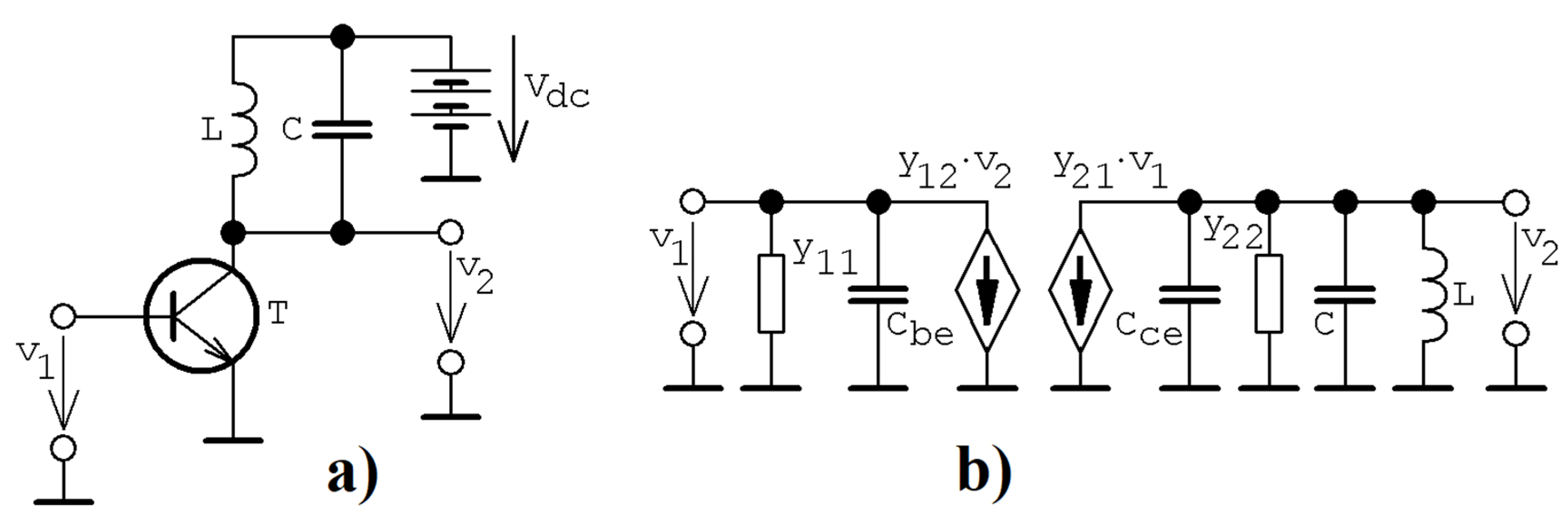
2. Simplest Model of Class C Amplifier

The fundamental structure of a single-transistor class C amplifier is provided in Figure 1a. This circuitry can be redrawn for the useful high-frequency signals (typically about tens or hundreds of MHz) by considering significant parasitic capacitances, as shown in Figure 1b. Note that at this point, the system is considered isolated, i.e., without an input signal. Dynamics of the resulting network can be described by following a set of ordinary differential equations:

$$C_1\frac{d}{dt}{v}_1=-y_{11}·v_1-y_{12}\left(v_2\right), C_2\frac{d}{dt}{v}_2=-y_{21}\left(v_1\right)-y_{22}·v_2-i_L, L\frac{d}{dt}{i}_L=v_2,$$

(1)

where a state vector is x = (v₁, v₂, i_L)^T, y₁₁ and y₂₂ are the input and output admittance of the bipolar transistor, and y₁₂ and y₂₁ are transconductance-type nonlinear smooth functions of the form

$$y_{21}\left(v_1\right)=a_1·v_1+a_2·{v_1}^3 , y_{12}\left(v_2\right)=b_1·v_2+b_2·{v_2}^3.$$

(2)

Note that nonlinearities are considered lower-order polynomials; i.e., approximations are valid in the close neighborhood of the calculated bias point. Fixed points are all real solutions of nonlinear algebraic equations dx/dt = 0, i.e.,

$$v_1=-y_{12}\left(0\right)/y_{11} , v_2=0, i_L=-y_{21}\left(v_1\right).$$

(3)

Therefore, Dynamical System (1) with (2) possesses only a single equilibrium located at zero. Associated eigenvalues can be established as roots of characteristic polynomial

$$s^3+\left(\frac{y_{11}}{c_1}+\frac{y_{22}}{c_2}\right)·s^2+\left(\frac{1}{c_2·l}-\frac{a_1·b_1}{c_1·c_2}+\frac{y_{11}+y_{22}}{c_1·c_2}\right)·s+\frac{y_{11}}{c_1·c_2·l}=0.$$

(4)

Small letters denote normalized values of circuit components. In general, Math Model (1) is analyzed using normalized values of accumulation elements and admittances. For a particular application, time and impedance rescaling need to be considered. Note that capacitor C₁ de facto represents parasitic capacitance between the base and emitter C_be, while C₂ is a sum of parasitic C_ce and tank capacitance. Detailed numerical investigations reveal the advantageous possibility to keep C₁ = C₂ = 1 F and L = 1 H. For further analysis, let us assume that linear term a₁ in Function (2) is very small. Symbolic formulas for eigenvalues can be expressed as

$${\delta }_1=-\frac{y_{11}}{c_1} , {\delta }_{2,3}=-\frac{1}{2·c_2}·\left(y_{22}\pm \sqrt{y_{22}^2-\frac{4·c_2}{l}}\right),$$

(5)

i.e., we experience a pair of complex conjugated eigenvalues if y₂₂²⋅l < 4⋅c₂. In this case, local vector field geometry near the origin is spanned by the eigenvector and eigenplane defined by two lines, namely

$$\begin{gathered} {ϵ}_{vector}={\left(\begin{array}{ccc}1& 0& 0\end{array}\right)}^T , \\ {ϵ}_{plane}^1=Re{\left(\mp \begin{array}{ccc}\frac{l·b_1·\left(y_{22}\pm \sqrt{y_{22}^2-\frac{4·c_2}{l}}\right)}{c_1·\sqrt{y_{22}^2-\frac{4·c_2}{l}}+2·c_2·y_{11}-c_1·y_{22}}& -\frac{l·\left(y_{22}\pm \sqrt{y_{22}^2-\frac{4·c_2}{l}}\right)}{2·c_2}& 1\end{array}\right)}^T, \\ {ϵ}_{plane}^2=Im{\left(\mp \begin{array}{ccc}\frac{l·b_1·\left(y_{22}-\sqrt{y_{22}^2-\frac{4·c_2}{l}}\right)}{c_1·\sqrt{y_{22}^2-\frac{4·c_2}{l}}+2·c_2·y_{11}-c_1·y_{22}}& -\frac{l·\left(y_{22}\pm \sqrt{y_{22}^2-\frac{4·c_2}{l}}\right)}{2·c_2}& 1\end{array}\right)}^T. \end{gathered}$$

(6)

Nonlinear scalar functions y₁₂(v₂) and y₂₁(v₁) have been considered as cubic polynomials without offset, while all remaining parameters were freely enabled for optimization. During the search procedure, the bipolar transistor was fixed in an active regime of operation where y₂₂ = 0 S. Therefore, fifth-dimensional hyperspace of the internal system parameters undergoes the optimization algorithm where the largest Lyapunov exponent (LLE) together with a simple condition for a bounded attractor has been combined and adopted as a fitness function. Finally, the following set of internal parameters was discovered:

$$y_{11}=0.42 , a_1=0 , a_2=1.2 , b_1=1.71 , b_2=-\mathrm{0.88.}$$

(7)

Using these values, eigenvalues near the equilibrium point form unstable geometry ℜ³∈ℜ²_unstable⊕ℜ¹_stable; i.e., the dynamical flow near the origin acts according to saddle-spiral vector field geometry. Eigenvalues are δ₁ = −0.486 and δ_2,3 = 0.033 ± j0.929.

Note that the final set of ordinary differential equations has eight terms, including two polynomials. Therefore, it does not belong to the family of the simplest chaotic flows, as discussed in papers [35,36,37].

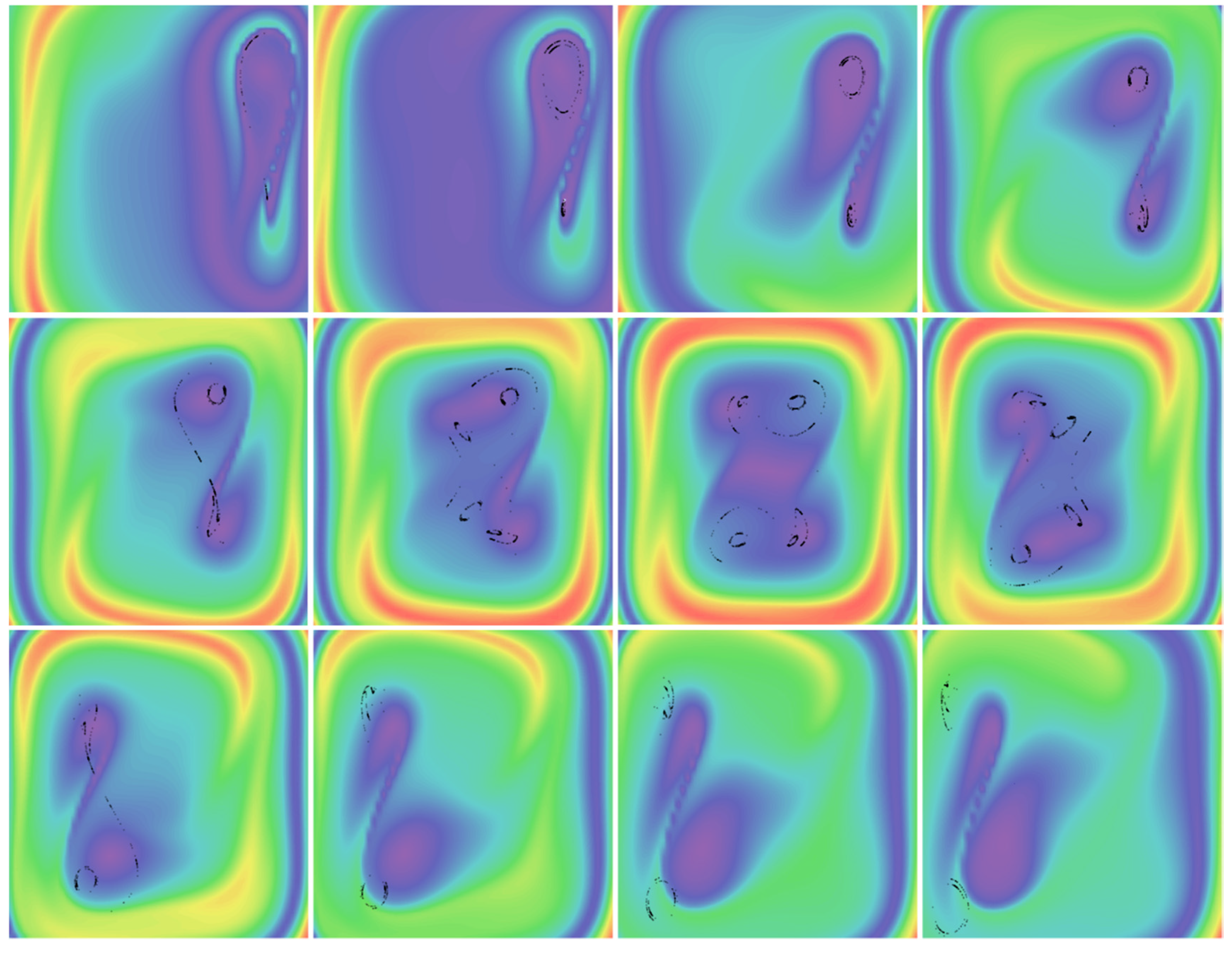
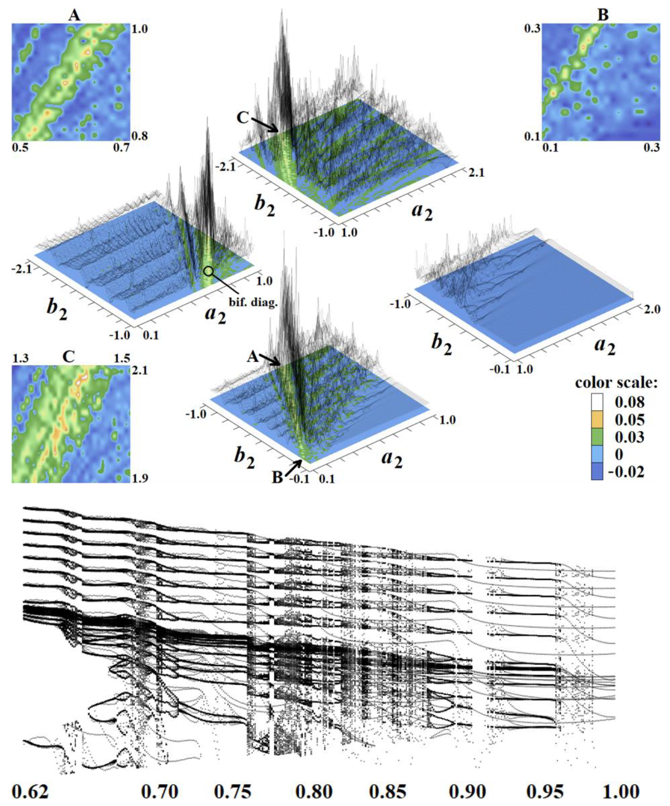
3. Numerical Results

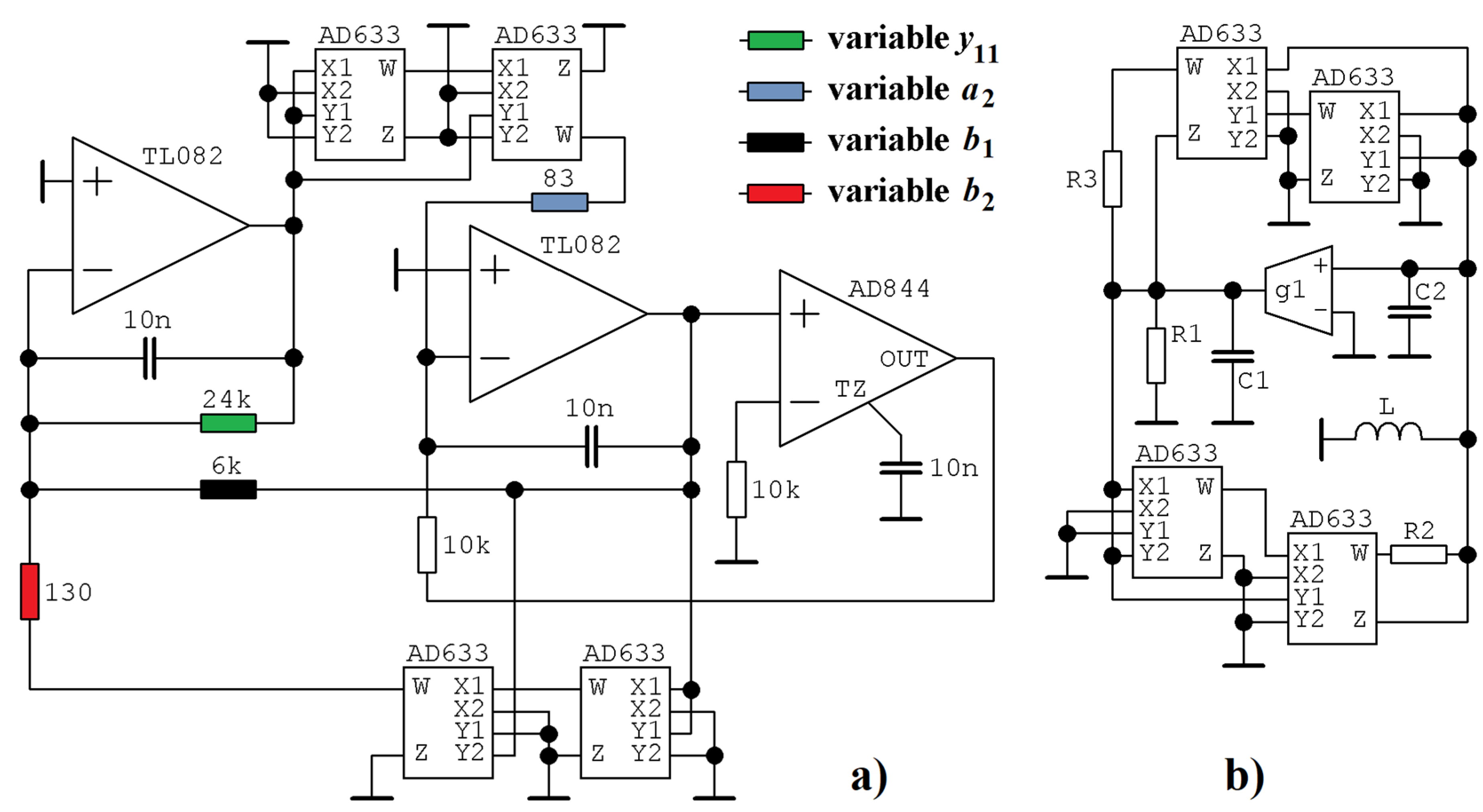
Discovered Novel Chaotic System (1) with Parameters (7) has been numerically analyzed using Mathcad and MATLAB. For numerical integration, the fourth-order Runge–Kutta method has been adopted. Figure 2 demonstrates the typical strange attractor generated by a bipolar transistor cell under bias point conditions mentioned above. The final time is 10⁴, time step is 10⁻², and sensitivity to changes in initial conditions is also visualized. The group of 10⁴ initial conditions were randomly generated around point x₀ = (1, 0, 0)^T using normal distribution with deviation of 10⁻² (red dots); short time evolutions after 1 s are plotted (blue), and then states after 100 s of the integration process are depicted (orange dots), and the final state after 1000 s is provided (green dots). Note that neighborhood state trajectories diverge slowly, and this should be respected when setting input parameters of the upcoming analysis. Figure 3 shows dynamic energy calculated in the state space volume where the strange attractor evolves. In this plot, a rainbow scale is used: red denotes high energy, green stands for average value, and blue marks regions with very low dynamic energy. Figure 4 illustrates basins of attraction for the typical chaotic attractor generated by a transistor-based system. Here, each plot contains a linear grid having 101 × 101 points, and the color scale is as follows: the limit cycle is marked by green, chaotic attractor by red, and fixed-point solution is blue. Ranges of horizontal and vertical axes are the same for each plot: v₁∈(−5, 5) and v₁∈(−5, 5), respectively.

Figure 5 provides us with an idea about potential robustness of the designed chaotic oscillator. This idea is simplified and plotted in two dimensions, namely as a function of cubic terms a₂ and b₂. This figure also illustrates zoomed plots A and C, where chaotic areas guarantee the generation of structurally stable strange attractors. However, careful circuit realization is still required for future laboratory success. The LLE was calculated using a final time of 10⁴, time step of 10⁻² s, and Gram–Schmidt orthogonalization. For each line in these three-dimensional plots, a bifurcation diagram can be calculated. Two interesting examples denoted by letters D and E are demonstrated. Note that evolution of trumpet attractors is not subject to a traditional period-doubling route to the chaos scenario. During the calculation of Figure 5, the maximal value of LLE is 0.082, and the Kaplan–Yorke dimension of the associated chaotic attractor is about 2.2.

4. Circuit Design

Synthesis of lumped chaotic oscillators based on knowledge of describing ordinary differential equations is a simple task with multiple solutions. The most straightforward approach is known as the concept of analog computers. Following this approach, only three basic building blocks are necessary: inverting integrators, differential amplifiers, and two ports with the prescribed nonlinear transfer curve. These circuits can be designed either in voltage mode [38,39] or current mode [40]. The first case is much more common because of the commercial availability of active elements and easily measurable state variables. The corresponding circuit implementation of the analyzed dynamical system is provided via Figure 6a, and its behavior is uniquely determined by the following set of ordinary differential equations:

$$C_1\frac{d}{dt}{v}_1=-\frac{v_1}{R_{green}}-\frac{v_2}{R_{black}}+\frac{K^2}{R_{red}}{v_2}^3 , C_2\frac{d}{dt}{v}_2=-\frac{v_3}{R_{brown}}-\frac{K^2}{R_{blue}}{v_1}^3 , C_3\frac{d}{dt}{v}_3=\frac{v_2}{R_{white}} ,$$

(8)

where C₁, C₂, and C₃ are the left, middle, and right capacitor, respectively. Note that seven active devices are needed for network design. The time constant is a compromise between the speed of integration (should be high due to long transients) and parasitic properties of active elements (should be low such that parasitic properties can be neglected). In our case, it is chosen as τ = 10⁴ × 10⁻⁸ = 100 μs. In the first experiments, red and blue resistors were supposed to be of variable values, i.e., potentiometers. Much better results were achieved if system dissipation also became an adjustable quantity, i.e., the green resistor was substituted by a potentiometer. It is worth noting that OrCAD PSpice circuit simulator has been used to validate the upcoming experimental results before construction of the oscillator.

The oscillator can be simplified by the following different idea. Assume that each differential equation represents the sum of the currents measured at independent nodes. One can easily obtain the electronic system visualized in Figure 6b and described by mathematical expression

$$C_1\frac{d}{dt}{v}_1=-\frac{v_1}{R_1}-g_1·v_2+\frac{K^2}{R_3}{v_2}^3 , C_2\frac{d}{dt}{v}_2=-i_L-\frac{K^2}{R_{blue}}{v_1}^3 , L\frac{d}{dt}{i}_L=v_2 ,$$

(9)

where K = 0.1 is the internally trimmed constant of a four-quadrant analog multiplier. Obviously, the number of active elements decreases to five. On the other hand, the third state variable is not easily measurable. Note that, without the introduction of state variable rescaling, transadmittance amplifier g₁ should be able to handle high input voltages without output current distortion.

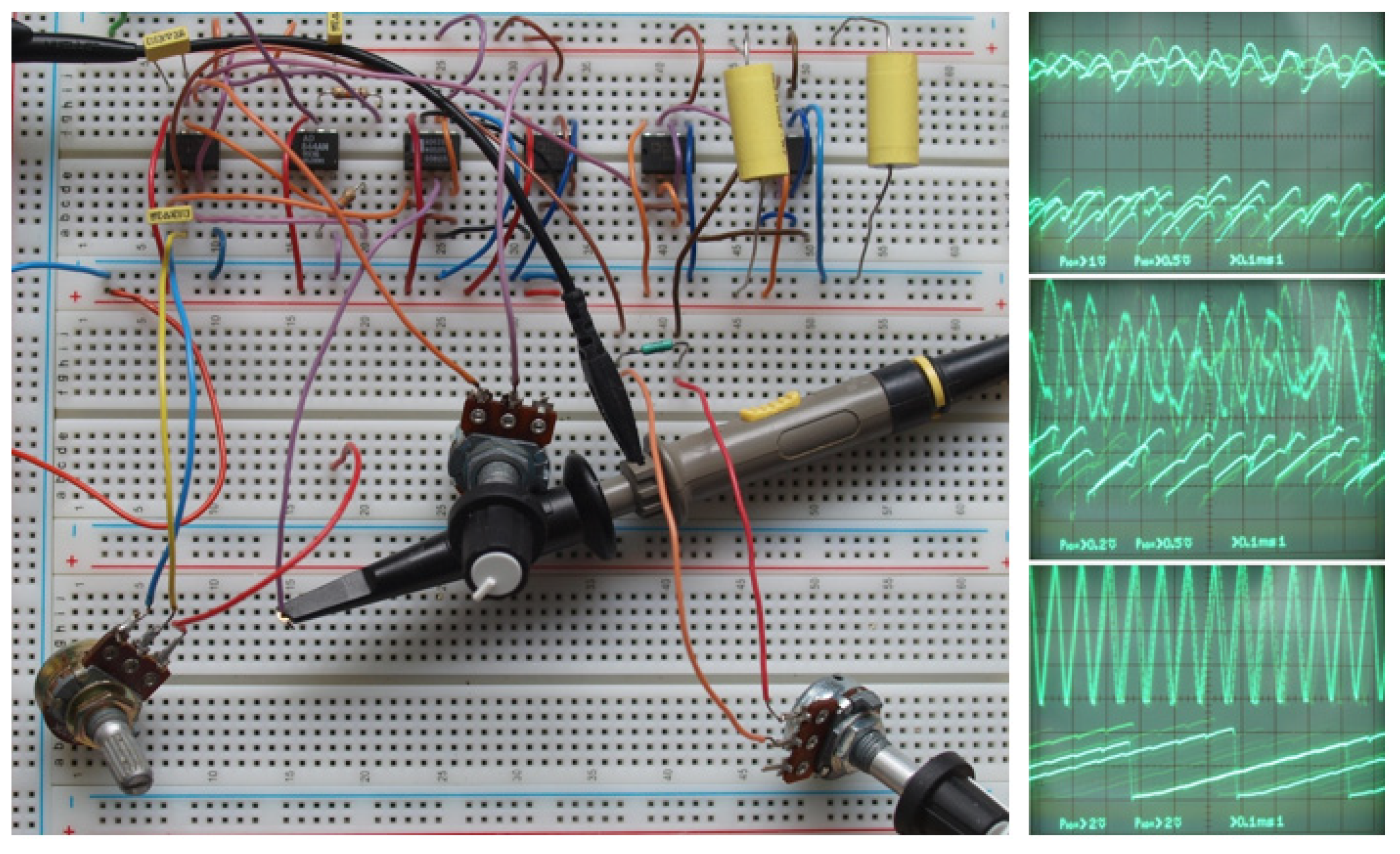
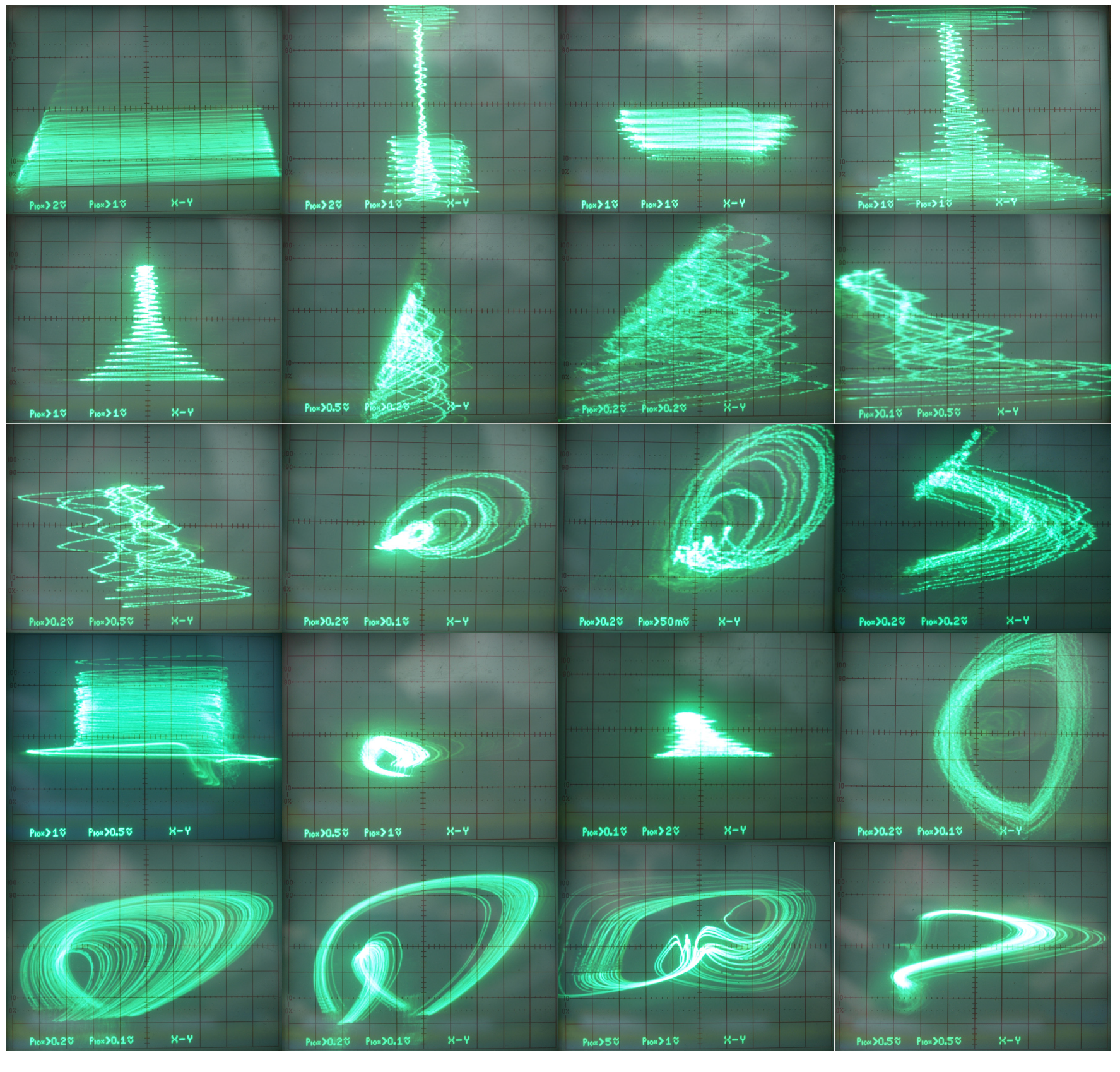
5. Experimental Verification

The new structure of the chaotic oscillator was designed using universal breadboard; see Figure 7, where the measurement setup is demonstrated. Interestingly, variously shaped strange attractors captured by oscilloscope during experimental verification of the proposed chaotic oscillator are shown in Figure 8. Some of them were not discovered during numerical analysis but were repeatedly observable within the dynamics of the lumped chaotic oscillator.

For given numerical values, the designed chaotic circuit generated waveforms with a continuous scale of the nonnegligible frequency components up to 100 kHz. Therefore, this oscillator can be used in many applications instead of truly random (noise) signal generators [41], to secure communication channels and information sources [42], as the core engine for chaos-based modulation and cryptography techniques [43], etc.

6. Discussion

The work described in this paper, that is, the discovery of chaotic dynamics within a generalized class C amplifier, leaves a significant place for future research activities. Let us mention a few unanswered questions and challenges:

(a)

The presence of chaos in the case of nonlinear transconductances approximated by piecewise-linear functions. From a circuit design point of view, the analog multipliers can be substituted by series and/or parallel connections of diodes.

(b)

The existence of chaos in a class D single-transistor-based amplifier. Three degrees of freedom required for chaos evolution are presented in fundamental topology (thanks to an output LC low-pass passive filter) without need of considering intrinsic parasitic capacitances of the transistor itself.

(c)

Robust chaos detected in Figure 1b under the condition of linear y₁₂(v₂), i.e., the only nonlinear function in the mathematical model stands at y₂₁(v₁).

This list is by no means complete. Further interesting reading about chaotic circuits having one or two bipolar junction transistors can be found in [44].

7. Conclusions

This popularizing paper represents a simultaneous contribution to two areas of chaos theory: (a) the discovery of a new chaotic dynamical system with a specific type of equilibria, namely a single unstable fixed point, and (b) the numerical description of a very simple single-transistor-based network structure from the viewpoint of chaos evolution.

The analyzed amplification topology can be commonly found in many complex electronic systems. The formation of strange attractors is conditioned by the non-unilateral nature of the bipolar transistor; backward trans-conductance especially needs to be active. Typical values of admittance parameters depend not only on the bias point but also on the transistor used. Unipolar transistors are usually modeled differently: by input admittance y₁₁ and trans-conductance y₁₂ equaling zero. However, matching circuits can cause feedback required for chaos evolution. In such a situation, chaos can be observed also in the case of a class C amplifier with a field-effect transistor. Matching networks with accumulation elements will increase the order of the final circuit; i.e., the probability of chaos can be boosted as well.

Based on the findings provided in this paper, chaotic motion can be mitigated by unilaterization of a bipolar transistor, that is, by the reduction of its backward trans-conductance.

References

1. Delgado-Bonal, A.; Marshak, A. Approximate entropy and sample entropy: A comprehensive tutorial. Entropy 2019, 21, 541. [Google Scholar] [CrossRef] [Green Version]
2. Pincus, S.M. Approximate entropy as a measure of system complexity. Proc. Natl. Acad. Sci. USA 1991, 88, 2297–2301. [Google Scholar] [CrossRef] [PubMed] [Green Version]
3. Pincus, S. Approximate entropy (ApEn) as a complexity measure. Chaos Int. J. Nonlinear Sci. 1995, 5, 110–117. [Google Scholar] [CrossRef]
4. Wolf, A.; Swift, J.B.; Swinney, H.L.; Vastano, J.A. Determining Lyapunov exponents from a time series. Physica 16D 1985, 3, 285–317. [Google Scholar] [CrossRef] [Green Version]
5. Yao, T.-L.; Liu, H.-F.; Xu, J.-L.; Li, W.-F. Lyapunov-exponent spectrum from noisy time series. Int. J. Bifurc. Chaos 2013, 23, 1350103. [Google Scholar] [CrossRef]
6. Sprott, J.C. Chaos and Time Series Analysis; Oxford University Press: Oxford, UK, 2003; 507p, ISBN 978-0198508397. [Google Scholar]
7. Eckmann, J.P.; Ruelle, D. Ergodic theory of chaos and strange attractors. Rev. Mod. Phys. 1985, 57, 617–656. [Google Scholar] [CrossRef]
8. Grygiel, K.; Szlachetka, P. Lyapunov exponent analysis of autonomous and nonautonomous set of ordinary differential equations. Acta Phys. Polon. B 1995, 26, 1321–1331. [Google Scholar]
9. Benettin, G.; Galgani, L.; Giorgilli, A.; Strelcyn, J.-M. Lyapunov characteristic exponents for smooth dynamical systems and for Hamiltonian systems; a method for computing all of them. Part 2: Numerical application. Meccanica 1980, 15, 21–30. [Google Scholar] [CrossRef]
10. Pham, V.-T.; Ali, D.S.; Al-Saidi, N.M.G.; Rajagopal, K.; Alsaadi, F.E.; Jafari, S. A novel mega-stable chaotic circuit. Radioengineering 2020, 29, 140–146. [Google Scholar] [CrossRef]
11. Sprott, J.C. Elegant Chaos: Algebraically Simple Chaotic Flows; World Scientific: Singapore, 2010; 304p, ISBN 978-981-283-881-0. [Google Scholar]
12. Petrzela, J. Optimal piecewise-linear approximation of the quadratic chaotic dynamics. Radioengineering 2012, 21, 20–28. [Google Scholar]
13. Jafari, S.; Sprott, J.C.; Pham, V.-T.; Golpayegani, S.M.R.Z.; Jafari, A.M. A new cost function for parameter estimation of chaotic systems using return maps as fingerprints. Int. J. Bifurc. Chaos 2014, 24, 1450134. [Google Scholar] [CrossRef]
14. Delgado-Restituto, M.; Linan, M.; Ceballos, J.; Rodriguez-Vazquez, A. Bifurcations and Synchronization using an integrated programmable chaotic circuit. Int. J. Bifurc. Chaos 1997, 7, 1737–1773. [Google Scholar] [CrossRef] [Green Version]
15. Nazarimehr, F.; Jafari, S.; Golpayegani, S.M.R.H.; Kauffman, L. Investigation of bifurcations in the process equation. Int. J. Bifurc. Chaos 2018, 27, 1750201. [Google Scholar] [CrossRef] [Green Version]
16. Petrzela, J. Fractional-order chaotic memory with wideband constant phase elements. Entropy 2020, 22, 422. [Google Scholar] [CrossRef] [Green Version]
17. Matsumoto, T. A chaotic attractor from Chua’s circuit. IEEE Trans. Circuits Syst. 1984, 31, 1055–1058. [Google Scholar] [CrossRef]
18. Guzan, M. Variations of boundary surface in Chua’s circuit. Radioengineering 2015, 24, 814–823. [Google Scholar] [CrossRef]
19. Kennedy, M.P. Chaos in the Colpitts oscillator. IEEE Trans. Circuits Syst. 1994, 41, 771–774. [Google Scholar] [CrossRef]
20. Kvarda, P. Chaos in Hartley’s oscillator. Int. J. Bifurc. Chaos 2011, 12, 2229–2232. [Google Scholar]
21. Kilic, R.; Yildrim, F. A survey of Wien bridge-based chaotic oscillators: Design and experimental issues. Chaos Solitons Fractals 2008, 38, 1394–1410. [Google Scholar] [CrossRef]
22. Rajagopal, K.; Li, C.; Nazarimehr, F.; Karthikeyan, A.; Duraisamy, P.; Jafari, S. Chaotic dynamics of modified Wien bridge oscillator with fractional order memristor. Radioengineering 2019, 28, 165–174. [Google Scholar] [CrossRef]
23. Song, Y.; Yuan, F.; Li, Y. Coexisting attractors and multistability in a simple memristive Wien-bridge chaotic circuit. Entropy 2019, 21, 678. [Google Scholar] [CrossRef] [Green Version]
24. Petrzela, J.; Polak, L. Minimal realizations of autonomous chaotic oscillators based on trans-immittance filters. IEEE Access 2019, 7, 17561–17577. [Google Scholar] [CrossRef]
25. Endo, T.; Chua, L.O. Chaos from phase-locked loops. IEEE Trans. Circuits Syst. 1988, 35, 987–1003. [Google Scholar] [CrossRef]
26. Hamill, D.C.; Jeffries, D.J. Subharmonics and chaos in a controlled switched-mode power converter. IEEE Trans. Circuits Syst. 1988, 35, 1059–1061. [Google Scholar] [CrossRef]
27. Zhou, X.; Li, J.; Youjie, M. Chaos phenomena in dc-dc converter and chaos control. Procedia Eng. 2012, 29, 470–473. [Google Scholar] [CrossRef] [Green Version]
28. Fossas, E.; Olivar, G. Study of chaos in the buck converter. IEEE Trans. Circuits Syst. I Fund. Theory Appl. 1996, 43, 13–25. [Google Scholar] [CrossRef] [Green Version]
29. Niu, Q. Study on bifurcation and chaos in boost converter based on energy balance model. Energy Power Eng. 2009, 1, 38–43. [Google Scholar] [CrossRef] [Green Version]
30. Galajda, P.; Guzan, M.; Spany, V. The state space mystery with negative load in multiple-valued logic. Radioengineering 2008, 17, 19–24. [Google Scholar]
31. Petrzela, J. Multi-valued static memory with resonant tunneling diodes as natural source of chaos. Nonlinear Dyn. 2018, 93, 1–21. [Google Scholar] [CrossRef]
32. Petrzela, J. Strange attractors generated by multiple-valued static memory cell with polynomial approximation of resonant tunneling diodes. Entropy 2018, 20, 697. [Google Scholar] [CrossRef] [Green Version]
33. Petrzela, J. On the existence of chaos in the electronically adjustable structures of state variable filters. Int. J. Circuit Theory Appl. 2016, 11, 605–653. [Google Scholar]
34. Petrzela, J. Chaotic behavior of state variable filters with saturation-type integrators. Electron. Lett. 2015, 51, 1159–1160. [Google Scholar] [CrossRef]
35. Sprott, J.C. Some simple chaotic flows. Phys. Rev. E 1994, 50, 647–650. [Google Scholar] [CrossRef] [PubMed]
36. Sprott, J.C. Simplest dissipative chaotic flow. Phys. Lett. A 1997, 228, 271–274. [Google Scholar] [CrossRef]
37. Sprott, J.C. Some simple chaotic jerk functions. Am. J. Phys. 1997, 65, 537–543. [Google Scholar] [CrossRef]
38. Itoh, M. Synthesis of electronic circuits for simulating nonlinear dynamics. Int. J. Bifurc. Chaos 2001, 11, 605–653. [Google Scholar] [CrossRef]
39. Karimov, T.; Nepomuceno, E.G.; Druzhina, O.; Karimov, A.; Butusov, D. Chaotic oscillators as inductive sensors: Theory and practice. Sensors 2019, 19, 4314. [Google Scholar] [CrossRef] [PubMed] [Green Version]
40. Petrzela, J.; Gotthans, T.; Guzan, M. Current-mode network structures dedicated for simulation of dynamical systems with plane continuum of equilibrium. J. Circuits Syst. 2017, 27, 1–39. [Google Scholar] [CrossRef]
41. Sapuppo, F.; Llobera, A.; Schembri, F.; Intaglietta, M.; Cadarso, V.J.; Bucolo, M. A polymeric micro-optical interface for flow monitoring in biomicrofluidics. Biomicrofluidics 2010, 4, 024108. [Google Scholar] [CrossRef] [Green Version]
42. Itoh, M. Spread spectrum communication via chaos. Int. J. Chaos Theory Appl. 1999, 9, 155–213. [Google Scholar] [CrossRef]
43. Chien, T.; Liao, T.-L. Design of secure digital communication systems using chaotic modulation, cryptography and chaotic synchronization. Chaos Solitons Fractal 2005, 24, 241–255. [Google Scholar] [CrossRef]
44. Minati, L.; Frasca, M.; Oswiecimka, P.; Faes, L.; Drozd, S. Atypical transistor-based chaotic oscillators: Design, realization, and diversity. Chaos 2017, 27, 073113. [Google Scholar] [CrossRef] [PubMed]
Figure 1. Bipolar transistor circuits: (a) principal concept and (b) equivalent circuit for high-frequency band.
Applsci 10 05025 g001
Figure 2. Numerical integration outputs: (a) typical double-trumpet chaotic attractor, (b) sensitivity to the changes in initial conditions, (c) zoomed short time evolution, (d) zoomed average time evolution, and (e) initial conditions close to point x0 = (0, 0, 0)T. Note the different scales of the axis system for individual plots.
Applsci 10 05025 g002
Figure 3. Kinetic energy calculated in horizontal slices of state space (from left to right, up to down) and return maps (black dots): z = −13, z = −10, z = −6, z = −3, z = −2, z = −1, z = 0, z = 1, z = 2, z = 3, z = 4, and z = 5.
Applsci 10 05025 g003
Figure 4. Basins of attraction calculated as horizontal slices of a state space: (a) iL = 0, (b) iL = 0.1, (c) iL = 0.2, (d) iL = 0.5, (e) iL = 0.7, (f) iL = 0.8, (g) iL = 1, (h) iL = 1.5, (i) iL = 2.0, (j) iL = 2.5, (k) iL = 3.0, (l) iL = 3.5, (m) iL = 4, (n) iL = 4.5, (o) iL = 5, (p) iL = 6, (q) iL = 8, (r) iL = 10, (s) iL = 11, and (t) iL = 12.
Applsci 10 05025 g004
Figure 5. Topographically scaled surface-contour plot of LLE as a two-dimensional function of cubic terms associated with nonlinear transconductances y12(v2) and y21(v1). Bifurcation diagram fitted to the trumpet attractors; cross section chosen as v2 = −1.5 V, while state variable v1 is stored.
Applsci 10 05025 g005
Figure 6. Two flow-equivalent practical realizations of chaotic oscillators based on a class C amplifier: (a) using the integrator block schematic and (b) directly following Kirchhoff’s first law.
Applsci 10 05025 g006
Figure 7. Detail photo of the chaotic oscillator realized using universal breadboard; generated chaotic waveforms in time domain visualized using an oscilloscope.
Applsci 10 05025 g007
Figure 8. Selected oscilloscope screenshots (plane projections of strange attractors) captured during experimental measurement; specific values of system parameters (slider positions of potentiometers) are not provided.
Applsci 10 05025 g008aApplsci 10 05025 g008b