A Novel Grid and Place Neuron’s Computational Modeling to Learn Spatial Semantics of an Environment

Abstract

Health-related limitations prohibit a human from working in hazardous environments, due to which cognitive robots are needed to work there. A robot cannot learn the spatial semantics of the environment or object, which hinders the robot from interacting with the working environment. To overcome this problem, in this work, an agent is computationally devised that mimics the grid and place neuron functionality to learn cognitive maps from the input spatial data of an environment or an object. A novel quadrant-based approach is proposed to model the behavior of the grid neuron, which, like the real grid neuron, is capable of generating periodic hexagonal grid-like output patterns from the input body movement. Furthermore, a cognitive map formation and their learning mechanism are proposed using the place–grid neuron interaction system, which is meant for making predictions of environmental sensations from the body movement. A place sequence learning system is also introduced, which is like an episodic memory of a trip that is forgettable based on their usage frequency and helps in reducing the accumulation of error during a visit to distant places. The model has been deployed and validated in two different spatial data learning applications, one being the 2D object detection by touch, and another is the navigation in an environment. The result analysis shows that the proposed model is significantly associated with the expected outcomes.

1. Introduction

In robotics, the robust localization on an object is very crucial in the perspective of physical tasks. Specifically, in navigation, the localization and path integration is really a big issue over which several efforts have taken place for more than 20 years [1,2,3]. The very first approach proposed for the localization of an agent was the extended Kalman filter (EKF) [4]. The complexity of EKF is quadratic with respect to the landmark’s number, and thus, it behaves badly in a large environment [5]. The localization is also crucial for the object handling tasks, where body motion integration is required with a cognitive map of an object. Several other cognitive tasks can be done using body motion integration like picking an object, recognizing an object by touch, etc. In the context of object-handling tasks, the work is surely not appropriate. In human brain research, it has been well established that the collaborative network of grid and place cell neurons are responsible for learning the spatial semantics of an environment/object. Moreover, the network integrates the body motion with the learned semantics and helps a human in localization within an environment/object [6,7,8,9,10,11,12,13,14,15,16]. Using such localization, a human does several physical tasks. Several bio-inspired modeling works have been published on localization that has used the general idea of grid cell neuron. RatSLAM (Simultaneous localization and mapping) [17] is the most popular among all. The model has shown the localization using a 3D continuous attractor network of pose cells. The size of the network used in the model is dependent on the size of the environment; therefore, the model is highly infeasible for large environments.

Numerous computational models of grid neurons have been published since 2005 that have generated the hexagonal grid patterns, like the continuous attractor [18] and oscillatory interference model [18], and hybrid oscillatory attractor network [19,20]. However, the models have not addressed the problem of ambiguity in the interference of several grid patterns. Due to ambiguity, an agent can localize to the wrong place and direction. In the direction of modeling a place neuron, a new robotic architecture has merged the visual place cell with the grid cell to limit the angular drift of the path integration [21]. Despite a huge amount of theoretical models, none of the models has used the grid neuron and the place cell activities in performing the object-handling tasks. Moreover, the grid and the place cell neurons play a crucial role in the episodic memory as well [22,23,24]. As an episodic memory makes use of a place cell neuron in learning of procedures for making and recalling, predictions, and planning. Although the robots in current scenarios are using advanced sensors and advanced vision techniques to make actions [25,26,27,28,29,30,31,32], still the techniques are so erroneous. Somewhere, we need body object integration along with the advanced vision and sensors for the smooth functioning and it may have many applications in machine learning, smart grids, and the energy sector [33,34,35,36,37,38,39,40,41,42].

The article proposes a quadrant model for the grid neuron and an interference model for the place neuron modeling to address the aforementioned shortcomings and the existing research gaps of grid modeling. The quadrant model can generate the periodic hexagonal grid pattern from the navigational input of an artificial agent. Furthermore, an interaction system of place and grid neuron has also been proposed that can learn the cognitive map of an environment. The cognitive map learning is done using the integration of a quadrant grid neuron’s activation pattern with the associated sensation of a place neuron. The proposed computational mechanism for the place neuron is able to localize the agent correctly in the mental representation of space and provides the ability to do path integration as well. Furthermore, a place sequence learner is proposed in this research work that learns the sequence of places in the context of current and goal locations. The learned trip gives the information of the next nearby locations and the associated grid code and other learned parameters to reach the destination. Since each trip is forgettable based on the frequency of their use, it is also space-efficient. Finally, the proposed mechanism deployment of the model is shown in two different applications, one being the object detection by touch, and the second is the navigation.

The rest of the paper is organized as follows. Section 2 discusses the modeling challenges. Section 3 describes the proposed computational modeling work of the grid and the place neuron. Also, the deployment of the proposed work is shown in different applications in Section 4. Experimental results are illustrated in Section 5. Finally, the paper is concluded in Section 6.

2. Issue and Modeling Challenges

The most obvious challenge in the grid neuron modeling is to generate the periodic hexagonal grid patterns of different scales and orientations from body movement input. The grid neuron activation is shown in the Figure 1.

The neuron is like a bulb that turns on only when the agent comes within the firing range (grid ring); otherwise, it remains off. The firing locations constitute the hexagonal grid pattern. The firing intensity of the neuron inside the rings depends on the distance of the agent from the center of the ring. At the center, the neurons firing intensity will be the highest and vice versa. Each grid neuron possesses different orientations and spacing of firing locations. In Figure 2, the hexagonal grid pattern of different spacing and orientation is shown.

As per the biological brain research, the grid neuron works in collaboration with the place neurons. The connectivity between the grid and the place neuron is shown in Figure 3. The place neuron learns the grid neurons activation value through forward connectivity and in turn activates the grid neurons during localization through backward connectivity.

The task of a place neuron is to learn a unique location of a cognitive map in terms of code as it is activated in a single location in an environment [15,21]. The challenge in the modeling of a place neuron is to learn the interference pattern of grid neurons without any ambiguity. The interference of two different activation patterns is shown in Figure 4, where a location is associated with a unique combination of the activations of two different grid neurons. If a place neuron simply learns the activation values of grid neurons as a grid code, then there can be the possibility of ambiguity. The case of ambiguity is shown in Figure 5, in which the two different interference patterns are shown correspond to the same grid code.

In previous works on navigation, a robot always considered as a single entity, but in the case of object handling tasks, there is a need to consider the motion of each individual body part. The integration of the sensory perception of each individual body part in a single semantic map of an object is a challenging task.

3. Proposed Mechanism

The article proposes a quadrant-based mechanism for the modeling of grid neurons to address the aforementioned problems. The mechanism generates the periodic hexagonal grid pattern. Furthermore, an interaction system of place and grid neurons is proposed to learn the cognitive map of an environment. Moreover, the deployment of the model is shown in context to different applications. The detailed description of each proposed mechanism is given below.

3.1. Movement Representation

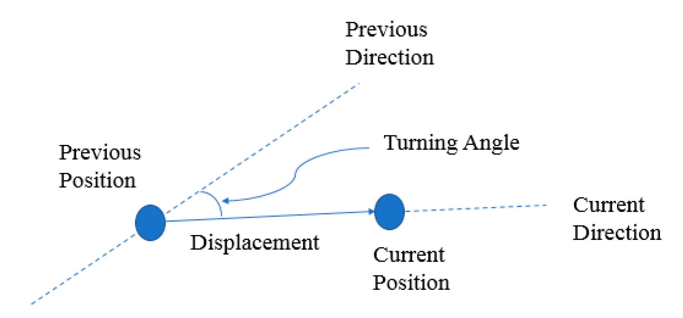
In the case of navigation, the entire body of an agent has been considered a unit. The agent movement is defined as the turning angle and the displacement, as shown in Figure 6. The turning angle is defined as the angle between the previous direction of movement and the direction of the current movement. The distance between the current and the previous location of the agent is defined as displacement.

3.2. Quadrant Model for Grid Pattern Generation from the Body Movement

To track the agent for firing a grid neuron, we have used a reference grid point that keeps tracking the agent coordinate in both x and the y dimension. Initially, while learning an environment, the starting location will be the location of the reference points of all grid neurons. The reference grid point is not having any physical coordinate. Instead, it is just a logical concept that keeps tracking the distance and the direction of the agent until the grid neuron fires. The grid neuron fires only when the agent enters within the vicinity of any other grid point or in any grid ring of the grid neuron. When the grid neuron fires, the reference grid is reset to the new values of the agent tracking parameters. The new values will be calculated with respect to the grid point under whose grid ring the agent is entered.

Each grid ring’s center (i.e., the grid point) has a certain relationship with its surrounding grid rings center due to the periodicity of the firing pattern (calculation is shown in Section 3.2.2). The relationship allows any reference grid point to check whether the agent is entered into the vicinity of any of its surrounding grid point/grid ring or not. The relationship will be in terms of measured distances along both dimensions (i.e., x and the y-axis) from the reference grid point. Whenever the agent’s measured distances along both dimensions follow the relationship similar to any of the surrounding grid points of the reference grid point, then the grid neuron will be fired. The grid point whose relationship is matched with the agent will be considered as a new reference point. The old tracking parameters will be reset to the new tracking parameters, i.e., the measured distance of the agent from the newly recruited reference point. The same process will be repeated again and again until the agent stops movement.

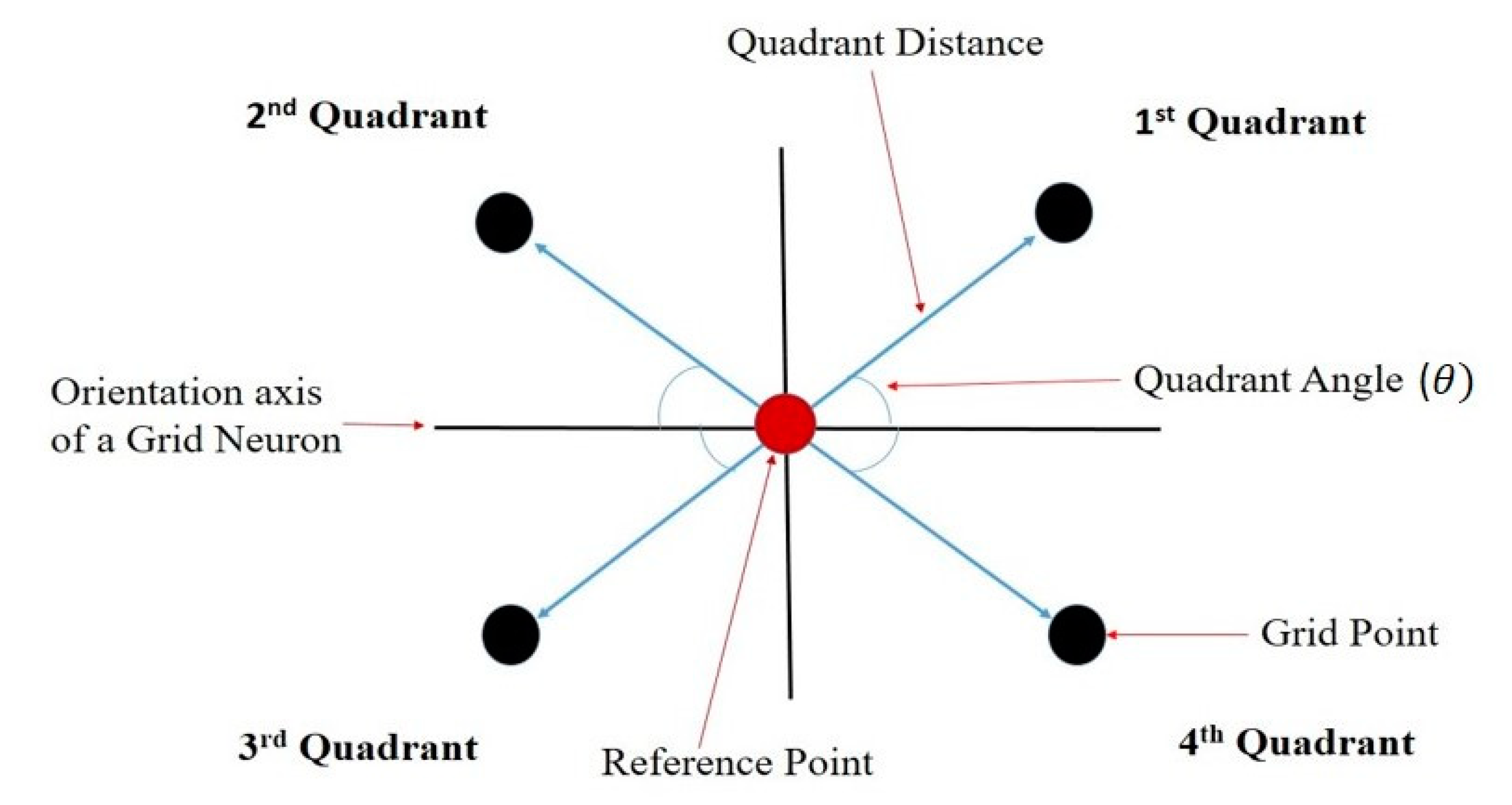
Since the reference ring is not always the origin, therefore the agent can move any of the four quadrants of the reference ring. Due to symmetry, the relation of the reference ring with the surrounding grid rings is similar in all four quadrants, as shown in Figure 7. Every grid ring has a corresponding grid ring in all other quadrants, which has the same distances along both dimensions. The signs of the agent’s coordinates tell the current quadrant number. The sign of the coordinates will be ignored while matching with the surrounding grid rings as the grid rings follow the same relation in all quadrants.

3.2.1. Finding the Coordinates of the Agent Based on the Magnitude and the Current Direction of Movement from a Reference Point

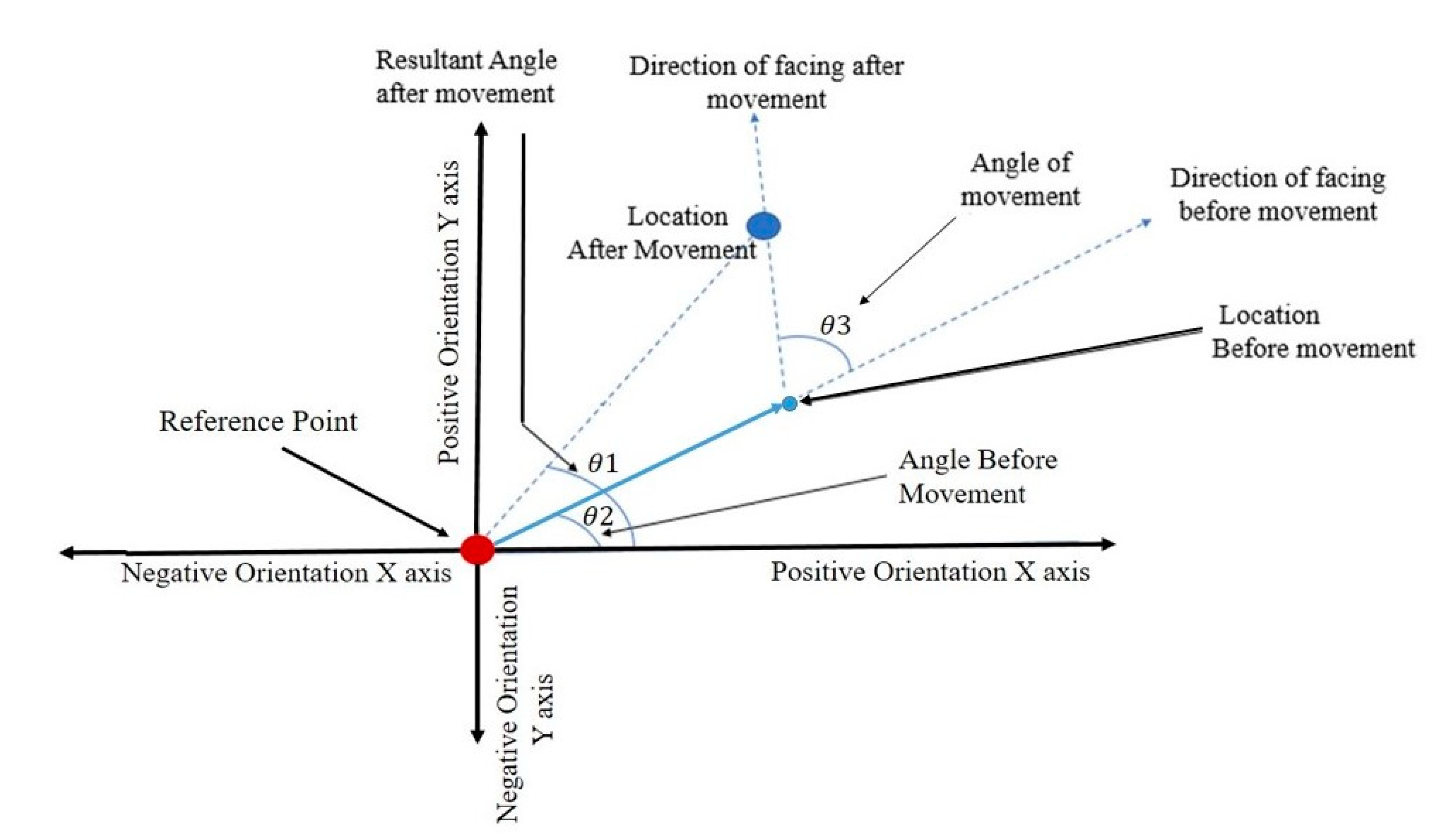
The calculation of the agent’s coordinate with respect to the reference grid point is shown below as Algorithm 1. The parameters used in the algorithm are illustrated in Figure 8. The parameter “$\theta 3$” tells the rotation of the agent’s body in degree, “Direction” is the direction of movement, that is having two possible values, one is left another is the right, “$\theta 2$” is the quadrant angle before movement and “$\theta 1$” is the quadrant angle after movement.

$$\theta 1=\{\begin{array}{c}\theta 2+\theta 3, |\mathrm{Direction} == \mathrm{LEFT}\\ \theta 2-\theta 3, |Otherwise\hfill \end{array}$$

(1)

$$\mathrm{X}\_\mathrm{coordinate}=\mathrm{X}\_\mathrm{coordinate}+(\mathrm{magnitude}\times \cos (\theta 1\left)\right)$$

(2)

$$\mathrm{Y}\_\mathrm{coordinate}=\mathrm{Y}\_\mathrm{coordinate}+(\mathrm{magnitude}\times \sin (\theta 1\left)\right)$$

(3)

3.2.2. Grid Neuron Activation

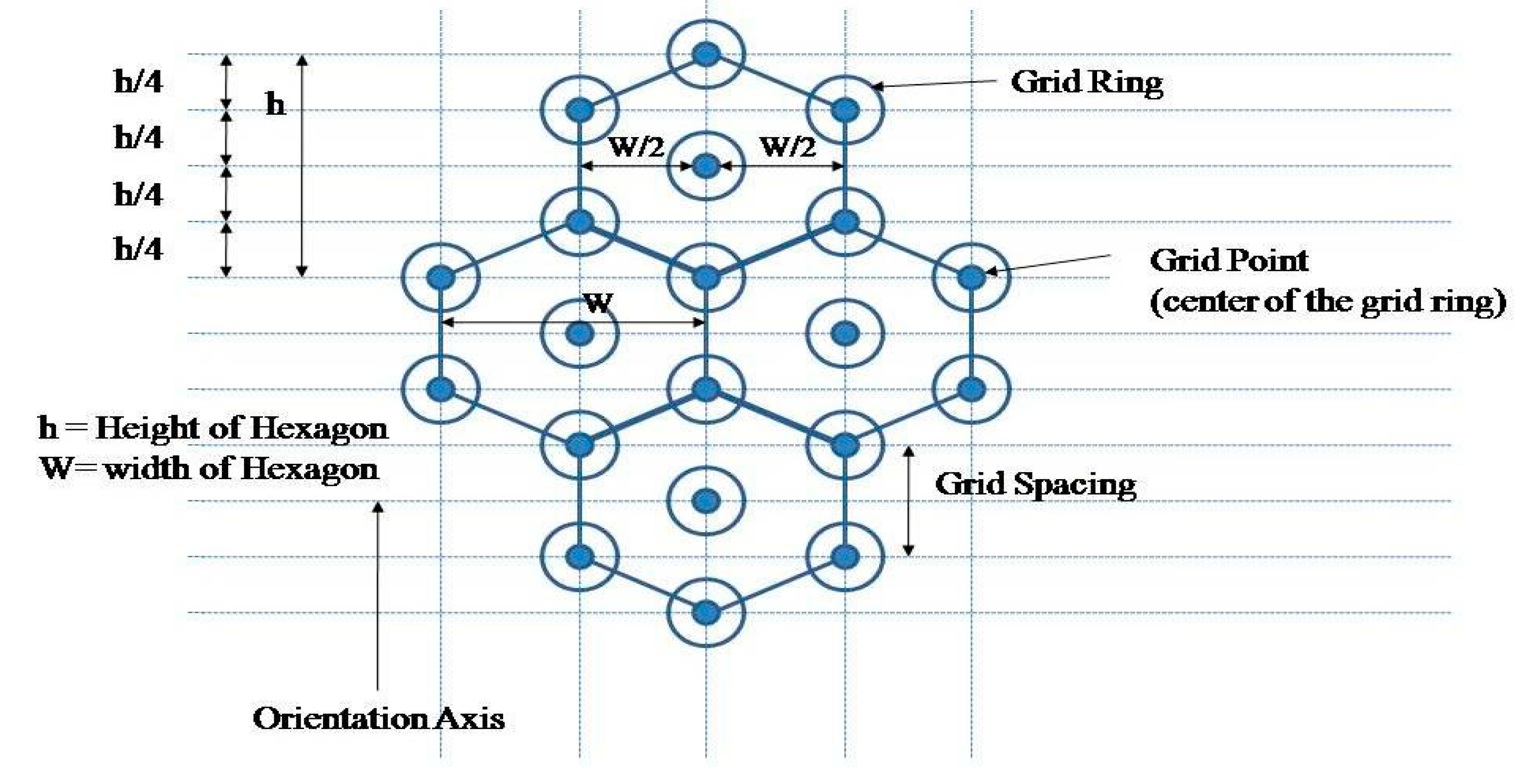
Generating a hexagonal grid like activation pattern needs to know the geometry of a hexagon which is shown below in Figure 9. In the figure, the distance between any two grid points sharing the same edge is of the same length, which is the grid spacing of a hexagon. There are two or more other parameters that describe the hexagon, which is the height and the width, whose calculations are shown in Equations (4) and (5). Parameters of the equations are illustrated in Figure 9.

Height of a hexagon:

H = 2 × d

(4)

Width of a hexagon:

W= Sqrt (3) × d

(5)

where H is the height, W is the width, and d is the grid spacing of a hexagon.

Each grid point is having a specific relation with all other grid points of the grid pattern. If we consider any of the grid points as a reference point and measures the distance of all other grid points along the x and y-axis direction from the reference point, then we obtain two categories of grid points. First are those whose distance along the x-axis is the integer multiple of the width of the hexagon, and distance along the y-axis is the 0.5 multiple of the height. Second, are those whose distance along the x-axis is the (odd number/2) multiple of width and distance along the y-axis is the (odd number/4) multiple of height. In case the agent’s measured distance from the reference point follows any one of the above categories of the grid points, then it shows that the agent is at one of the grid points and as a result of this the grid neuron will be fired or activated with the activation value of 1. There can be a possibility that the agent lies within the grid ring of a grid point instead of a grid point. In that case, the grid neuron will be activated but the activation would be less than one and will be inversely proportional to the distance from the center of the grid ring which equals (1-D/R) where D is the distance from the grid point under whose firing range the agent is present, and R is the radius of the firing range. The value for the activation will be zero when the distance D is larger than R.

Since the grid points are infinite in a 2D space, therefore we need a mechanism that selects only a few grid points, to check whether the agent is within the vicinity of the grid point or not. As we know the relation of the grid points, therefore, it is easier to choose the grid points.

Here, two sets of grid points can be chosen. First are those grid points whose X coordinate (XCORD)is equal to the (W × ROUND (A^x/W)) and Y coordinate (YCORD) lie in the range from (H × (CEIL (A^y/H) − 1)) to (H × (CEIL(A^y/H)). The A^x and the A^y are the coordinates of the agent along the x and y-axis, respectively. The CEIL is a function that returns the smallest integer value that is bigger than or equal to a number, and ROUND is the round-off function that rounds off the value to the nearest integer.

Second are those in which x-axis coordinate of the grid point lies into the range from (ROUND (A^x/W) − 0.5) to (ROUND (A^x/W) + 0.5), and the y-axis coordinate would lie into the range of (FLOOR (A^y/H) + 0.25) to (FLOOR (A^y/H) + 0.75). Here, FLOOR is the largest integer function that returns the greatest integer less than or equal to a given number. The whole pseudo code to calculate the activation of a grid neuron is given below.

Algorithm 1: Calculation for the grid neuron activation

1:  I ← ROUND (XCORD/width)   // ROUND is the round off function

2:  J ← CEIL (YCORD/ H) −1    // CEIL is ceiling function

3:  while  J < CEIL (YCORD/H) do

4:        J ← J +0.5;

5:        Gx ← I × W// Gx is the X coordinate of the chosen grid point;

6:        Gy ← J × H// Gy is the Y coordinate of the chosen grid point;

7:        D ← EUCLIDEAN ((XCORD,YCORD), (Gx, Gy));

8:        // Euclidean to find the distance between agent and the chosen grid point

9:         if D < R then

10:          activation ← 1 − (D/R);

11:         else

12:          activation ← 0;

13:         end

14:         if Y is the 0.5 multiple of the height (h) then

15:          activation ← 1;

16:         else if X is the 0.5 multiple of the W(width) then

17:            If Y is the 0.25 multiple of the height (h) then

18:              activation ← 1;

19:             else

20:              activation ← 0;

21:             end

22:         end

23:  end

3.3. Grid Code Learning and ItsRecalling

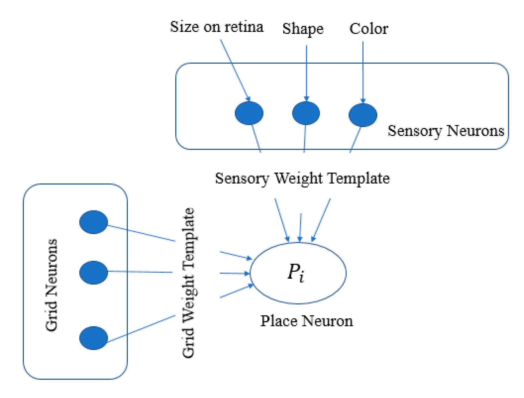
Here we hypothesized two states for a place neuron. One is the hyperpolarized state, in which a place neuron is always ready to learn the input grid neuron’s activation values. A place neuron comes in the hyperpolarized state only when the sensory input to the neuron matches with its sensory template, as shown in Figure 10 Another is the pseudo-polarized state in which the place neuron recalls their sensory template and matches it with the input sensory values. The pseudo-polarized state comes to the place neuron only when the input grid code matches the learned grid code of the place neuron. The pseudo-polarized state of a place neuron states the location of an agent in an environment.

Since similar grid activations can occur in many places in the environment, it is highly prone to error. Sometimes the grid neuron’s activation is not enough to tell the location, and this thing is shown in Figure 4 with example. Therefore, a place neuron needs to learn grid activations along with interference patterns of grid rings of different grid neurons. The interference pattern is a set of distances between the reference points of each grid neuron. The interference pattern is always unique in an environment, which is why it locates any area correctly in an environment, and the grid code states the exact location within the inferred area.

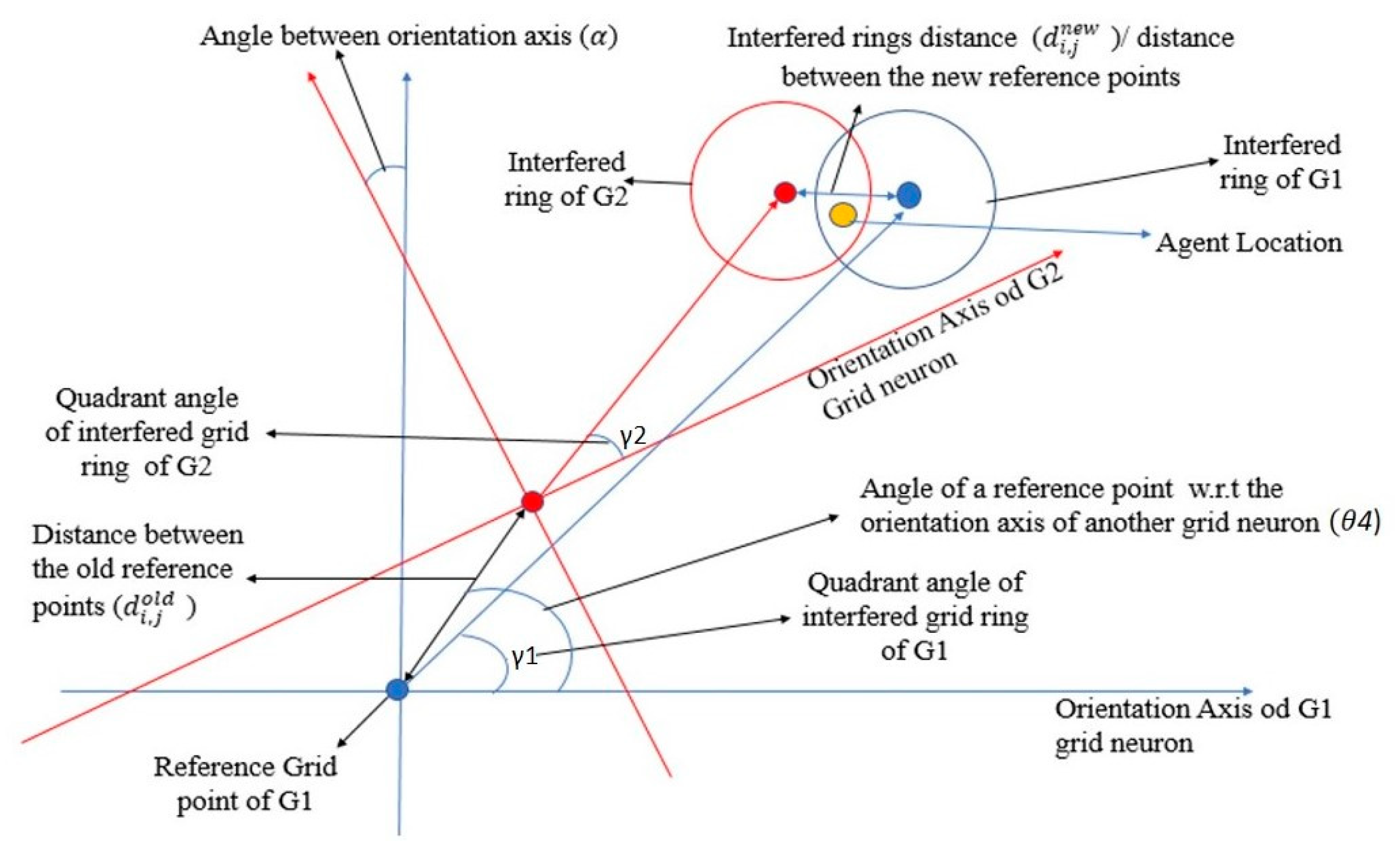
The interference of grid rings is shown below in Figure 11. In the figure, the blue-colored dots are representing the current reference points of their respective grid neurons. The orange-colored dot is representing the center of the firing field (grid ring) of a place neuron. The place neuron is present in the interference region of the grid rings. The yellow-colored dot represents the agent’s current location with regard to the interfered region of rings. The learning is necessary along with the grid point distances quadrant and the quadrant angles of every grid. Therefore, along with the reference points concerning learned place location, their orientation axis can also be recalled correctly, and that would help in further navigation after localization.

A place neuron can only be pseudo active when the agent enters the vicinity of a place neuron. The level of activation depends on the distance of the agent from the location of the neuron. Each place neuron calculates (for pseudo-activation) the match between their learned interference pattern with the agent’s current interference pattern as per Equation (6). The place neuron having the highest match will be the winner, and this winner place neuron recalls the distances of reference points and their activation values. The recalled values allow us to find their location with respect to all reference points of all grid neurons and then map the agent in the interference pattern to obtain their distance from the agent. Afterward, the place neuron will become pseudo active as per the Equation (7).

$$\begin{array}{c}winner=Max \left(m^k\right)\\ m^k={\displaystyle \sum _{\forall i,j \in Grid Neuron}}\frac{d_{i,j}}{n^2-n\left(1+2p\right)}\\ d_{i,j}=\{\begin{array}{c}\hfill 0, |L{D}_{i,j}\ne C{D}_{i,j}\\ \left(1-|Lac{t}_i-Cac{t}_i|\right)+\left(1-\left|Lac{t}_j-Cac{t}_j\right|\right), |Otherwise\end{array}\end{array}$$

(6)

where, LD (i,j) is the learned distance between the ith and jth grid neuron’s reference points. The CD is the current distance between the ith and the jth grid neuron’s reference point. Lact_i is the activation of an ith grid neuron while learning the place. ‘p’ is the number of grid neurons having activation is zero while learning. $m^k$ is the match score of a kth place neuron $d_{i,j}$ is the distance between the current and the learned interference pattern correspond to ith and jth grid neuron.

$$\mathrm{Pseudo}-\mathrm{activation}(\mathrm{i})=1-\frac{r}{r2}$$

(7)

where r1 is the calculated distance between the agent and the winner place neuron, r2 is the radius of the place neuron.

The mechanism of locating the agent and the place neuron with regard to the interference pattern is very simple. But, here there is a constraint, the location can be found only when the number of interfered rings is more than two. To find the location, from each reference point, draw a circle of radius proportional to the activation value, and then an intersecting point will be found, which will be the location of the place neuron, a similar process for the agent. This is how the distance between the agent and the place neuron can be calculated.

3.3.1. Calculation of Grid Point Distances of the Interfered Rings

In the aforementioned mechanism of place neuron activation, the mechanism of calculating the inter grid point distances is crucial and complex as well. The calculation of a distance between the centers of any two interfered grid ring is shown below in Equation (10). The parameters of the equation are illustrated in Figure 12.

$$X_j^{translated}=X_{j}Cos\alpha -Y_{j}Sin\alpha +(d_{i,j}^{old}\times \cos \theta 4)$$

(8)

$$y_j^{translated}=Y_{j}Sin\alpha -Y_{j}Cos\alpha +(d_{i,j}^{old }\times \sin \mathrm{e}\theta 4)$$

(9)

$$d_{i,j}^{new}=\sqrt{{\left(X_i-X_j^{translated}\right)}^2+{\left(Y_i-Y_j^{translated}\right)}^2}$$

(10)

where, $d_{i,j}^{old}$is the distance of the reference points of ith and jth grid neuron, $d_{i,j}^{new}$ is the calculated distance between the reference point of ith and jth grid neuron, $X_j^{translated}$ and $Y_j^{translated}$ are the translated X and Y coordinate of jth grid neuron into the coordinate system of another grid neuron (i.e., i), and $\propto$ is the angle between the orientation axis of interfered rings.

3.3.2. Role of Grid Spacing in the Localization Accuracy

The accuracy of localization depends not only on the number of grid neurons but also on the value of the grid spacing value of a participating grid neuron. The grid neuron has a large grid spacing fire only on 2–5 sites in an environment that helps in marking the sub-area in the environment where the agent is present. Whereas the grid neuron of smaller grid spacing fires from 50–80 sites in an environment that helps to locate the exact location in the marked sub-area. Therefore, we need to take both types of grid neuron in an appropriate ratio so that the accuracy can be increased, results related to this are shown in the result section.

3.4. Modelling of Place and Grid Neuron Interaction System to Perform Predictions and Recognition

The grid and place neurons deal with two types of information, one being the internal information, which is the movement of body parts like hand movement, eye movement (eye saccade). Second is the external information, which is the information observed by the human sensory organs. Here, grid neuron and place neuron interaction system are supposed to predict the external information based on the internal input information to recognize objects, environments.

The working of the proposed mechanism is shown in Figure 10. In the mechanism, the quadrant model (i.e., grid neuron) takes internal information as input, i.e., body movement. The interference model (i.e., place neuron) takes the input from the grid neurons (grid code) as well as from the sensory neurons (externally sensed information) through weighted connections. A place neuron is assumed to be an ART (adaptive resonance theory) network [22]. Here, a place neuron takes the input from several sensory neurons through weighted connections. The weight vector corresponds to a place neuron acts as its sensory template. The place neuron is activated only when the input sensory vector matches the template vector within the threshold limit. If none of the place neurons becomes activated, a new place neuron is recruited. The synaptic weights of the newly recruited neuron are initialized with the current sensory values. Moreover, the random grid neurons are connected to the newly recruited place neuron through weighted connections. The value of the weights of grid neurons associated with the recruited place neuron is initialized with the activation value of the grid neurons.

The mechanism of sensory information prediction is shown in Figure 13. The mechanism starts with the sensing of external information by the place neurons through the sensory neuron’s input. The place neuron matches within the threshold limit will be activated and recall their learned grid weight template. The grid weight template is the grid code that would tell the location in the environment or object. Once the agent obtains the location in the internal representation, it can generate the new grid code by the integration of recalled grid code with their body movement. The generation of new grid code would activate the place neuron whose grid weight template matches with the newly generated grid code (according to Equation (12)). The pseudo active place neuron will recall the associated sensory weight template, i.e., the prediction of sensory information from the body movement.

3.5. Place Sequence Learning

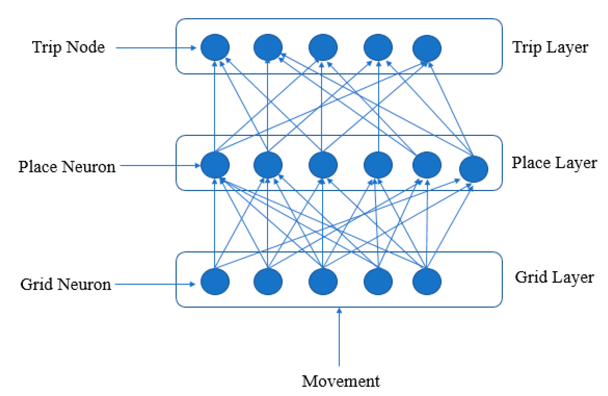
In hippocampal research, it has been found that the place neuron is activated earlier before reaching to the corresponding place of the place neuron. I also found the change in the activation pattern based on changing the current task and the goal location. This behavior shows the learning of the activation sequence of place neurons with respect to tasks or the goal location. Our proposed model has been incorporated with the same using the place sequence learner. The place sequence learner is shown in Figure 14. The sequence learner can recall the next sequential place neuron and its associated grid code. Since the recalled place neuron will always correspond to one of the neighboring places of the current activated one. Therefore, in navigation through neighboring place neuron’s grid code, the chances of error would be muchless. A place sequence learner is used to reduce the accumulation of errors while moving to a distant location. The learner recalls the grid code of the next place that is learned during the trip. The grid code can tell the movement direction exactly and the magnitude to obtain the location of the recalled grid code from the current grid code. Since the recalled place always is the local one in place sequence learner, therefore, the accuracy would be very higher compared to using the grid code of a destination place to move towards its corresponding place of the grid code.

Furthermore, a trip layer is used in sequence learners, which contains the neurons/nodes corresponding to each individual trip, which can be seen as an episodic memory of a trip. Here each trip is forgettable based on the frequency of recalling like the episodic events. Second is the place layer, which contains place neuron nodes. The third one is the grid layer contains the grid neurons. The grid layer nodes send the grid code to the place layer neurons, and the place layer nodes send the activation sequence to the trip layer nodes for learning. Each trip node has a weighted connection with each place neuron. The lowest is the weight earliest will be the position of the place neuron in the trip and vice versa. Initially, when the agent has not yet made any trip, no trip node will be there. With every new trip, a trip will be created whose weights with all place neurons will be initialized to zero;while navigation, the weight with the currently activated place neuron will be set to 1, and the weights with all other place neurons reduced by a factor (1 − β), as shown in the Equation (11).

$$\begin{array}{c}{W}_{i,j}=1\\ W_{i,k}=W_{i,k}(1-\beta )\hspace{1em}\forall k\ne j\end{array}$$

(11)

where, $W_{i,j}$ is the weight of jth place neuron with an ith trip node, j is the currently activated place neuron and β is the decaying factor.

During a visit to any goal location, the agent tries to find the trip node that is not having a null weight value with the goal location’s place neurons and the current location. If any such trip node is found, then it means that the trip is having a path from the current to the goal location. In case, if the weight value of the current place neuron is higher than the goal place neuron, then it shows that the path is from the goal to the current location, i.e., backward path. In the case of a forward path, the recalling starts with the place neuron having the next lowest weight value. In the case of the backward path, choose the next highest weight value. The process will be repeated until the place neuron correspondingto the goal location is recalled.

Trip strength is suggested to manage memory efficiently. If a trip frequently used, the trip strength for that trip increases with a learning rate; otherwise, it decreases. Let TS_i $ϵ$ [0, 1] be a trip strength for the ith trip node. The calculation for the trip strength is shown below in Equation (12).

$$T{S}_i\left(new\right)=\{\begin{array}{c}T{S}_{initial},Created\\ T{S}_i^{\left(old\right)}+\left(1-T{S}_i^{\left(old\right)}\right)r,Reactivated\\ \{\begin{array}{c}T{S}_i^{\left(old\right)}+T{S}_i^{\left(old\right)}{}^{{}^{(1-T{S}_i^{\left(old\right)}/\beta )}}\left(1-e\right),T{S}_i^{\left(old\right)}<1\\ T{S}_i^{\left(old\right)},T{S}_i^{\left(old\right)}==1\end{array}\},Otherwise\end{array}$$

(12)

where, β = 10, e is the emotion factor belongs to [0, 1] $T{S}_i$ is the memory strength of ith trip, which is initialized to the value of $T{S}_{initial}$ (0.5) at the time of trip creation and strength reinforces with each reactivation, r is the reinforcement rate, and strength decreased when the participated places of the trip get activated, and the event does not get reactivated. If TS_i falls below a threshold $\mu \in$ [0, 1], the ith trip node will remove from the memory.

4. Experimental Detail

The model is deployed in two different applications to assess the performance of the proposed mechanism, as discussed in the subsections.

4.1. Object Identification

In the experimental work of the object identification task, 100 different 2D objects have been taken. Each object is having a unique spatial allocation of sensations, i.e., each object is a permutation and combination of different sensations. The object is shown in Figure 15, where each sensation is represented by a unique color. Similar sensations are present in different objects but at different locations.

The object identification is made through navigating of fingers over the object whose results are shown in the results section. Three sensors are placed on each finger, whereas one of the sensors is considered as a base sensor. At every movement, each sensor generates a grid code in a parallel way. Each sensor except the base sensor generates the grid code from the current grid code of base sensor and its relative position from the base sensor.

This parallel exploration of any environment reduces the number of palm movements in learning and recognition as well.

If the size of an individual sub-region in a 2D object is bigger, then multiple grid codes can be allocated to the same sensation. As a result of that, during the recognition by touch, the observed sensation from a sub-region can recall multiple grid codes. The multiple grid codes create ambiguity in making the comparison. The ambiguity problem can be solved using the following steps:

• Observe the sensation of the base sensor, and recall the grid code corresponds to the observed sensation.
• Other sensors observe their sensations and recall their corresponding grid codes called sensed grid code.
• Next, each sensor integrates their relative position of the base sensor with the grid codes of base sensors to generate new grid codes called path integrated grid code.
• The next comparison will be made between the path integrated grid codes and the sensed grid codes. Those sensed grid codes found similar will be chosen to activate their associated place neurons.
• The objects which are associated with the activated place neurons will be in the list of the active object, and others will be inhibited for future activation.
• A similar process will be repeated again and again until a single object survives in the activation list.

4.2. Prediction during Navigation, and Navigation towards a Goal Location

Here place decoding mechanism is followed to self-localize (current location) in the internal representation of the environment. Further localization, there are two ways to reach the goal location. The first is through tracking the goal grid code. The second is the use of the trip to get the path consists of place sequence between the current and the goal location grid codes.

In the first way, there is a need to find the direction and distance of the goal location with regard to the current grid code. The mechanism is described below in the next Section 4.2.1.

While navigatingtowards the goal location, obstacles may occur. The agent can avoid the obstacles using the monocular image depth processing [32]. The depth image suggests the direction of a clear path, as shown in Figure 16. Figure 16a representing the environment’s original image. Figure 16b representsthe processed depth image. In the monocular depth image of an environment, objects that are in color closer to orange represents the obstacles or the objects that are closer to the agent, whereas the objects in colors closer to violet represent that the object is far from the agent. The agent always chooses the direction of violet color to move forward in the environment

The experimental environment has been created in UNITY, which is a 3D space where walls are placed to create an environment. The monocular depth processing [32] is used to find the obstacles in the path of the agent.

4.2.1. Finding the Direction of a Goal Location

By using the mapping as mentioned above of the environment into a grid code, the agent can obtain both current and the goal grid code. But here, the agent does not know which direction to choose to move forward so that the goal grid code can be reached. The agent solves this problem while it finds the activation grid points, which are closer to the current activation site for each participated grid neuron. The direction in which the overall match between the activation of each grid neuron with their corresponding activations in the goal grid code will be chosen by the agent to move forward. If none of the directions gives the match higher than the threshold, then test for the next activation site, first change the lowest scale grid neuron.

For all participated grid neurons in all directions, the direction in which the distance between the activation of each grid neuron founds closer to their corresponding activation goal grid code (as shown in Figure 17) will be the direction of movement for the agent. But in real scenarios, mostly the goal location will be hidden to the agent. Therefore, the agent needs to consider the walls, objects encountered in the path of the agent, which can change the direction of movement. Here, image depth is used to find out whether an object or the wall is there or not in the path if anything is encountered then the agent would change their direction to move forward and recalculate the direction.

4.2.2. Navigation Using Place Learner

The chances of error can be very high if the agent chooses grid codes to move toward the distant goal grid code. The calculation of the correct direction of a distant goal location can be error-prone due to ambiguity. Instead, an agent can search for the nearby locations/grid codes repeatedly to move towards a goal location. The mechanism would be less error-prone and more accurate in navigation. Which nearby grid code to choose will be obtained through a learned trip having both the current and the goal location in their learned sequence.

5. Results and Discussion

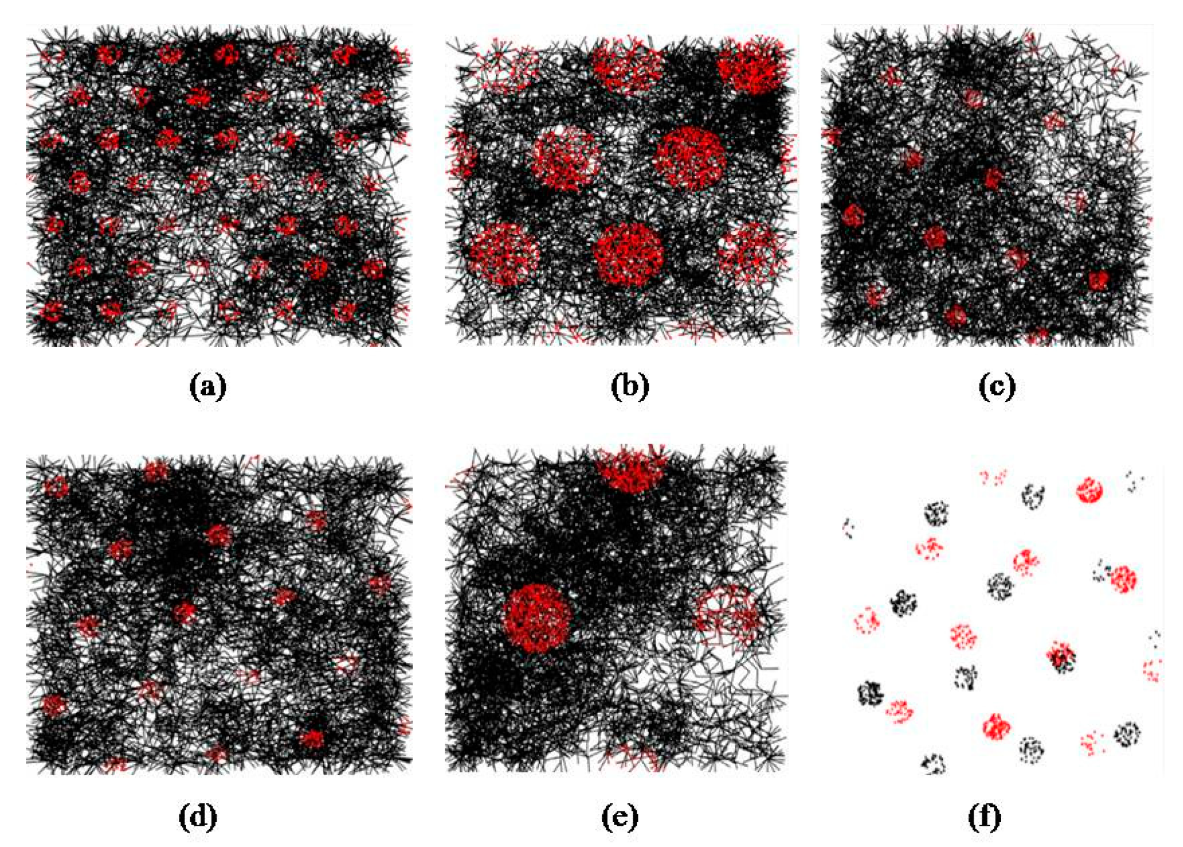
The experimental tests were carried out using the artificial agent in an environment of size 100 × 100 cm² for validating the proposed quadrant model. Here, the step size of the movement of the agent was fixed, but it could move in all directions randomly. The different grid patterns of different scales and orientations generated during different walks are shown in Figure 18.The trajectory of the agent is shown using black color and the red color showing the firing locations of a grid neuron. The observed firing locations in the figure constituted the perfectly periodic hexagonal grid pattern as expected.

Similarly, in the place neuron results, shown in Figure 19, the activation of a place neuron is perfect, and they have shown excellent silence in all over the field except the activation field of the place neuron (no false positive).

The experimental detail of different grid patterns shown in Figure 18 are as follows: (a) grid pattern generated corresponding to the 2000 steps of the agent, where the grid spacing is of 15 units and the radius of the grid circle is of 3 units; (b) representing the grid pattern corresponding to the grid spacing of 35 unit, where the radius of the grid circle is of 10 units; (c) spacing of 25 units, radius 3 units and orientation of 30 degrees; (d) spacing of 25, radius 3 unit and orientation of 10 degrees; (e) spacing of 55 and radius of 10unit, the orientation of 0 degrees; (f) representing the overlapping of firing patterns of two different grid neurons.

The result for the grid code is shown in Figure 20, where, the activations of 20 different grid neurons are shown using the heat map corresponds to a random location, whose coordinates are mentioned in the figure.

The performance of the proposed place and grid neuron interaction system is assessed in the task of object recognition and navigation. The results of the proposed model with regard to the different model parameters are given in the below subsections.

5.1. Results of Object Recognition

Since each object is a permutation of spatial sensations, therefore in the initial touch, the observed sensation will be present in almost every object. In the initial touch, every object will be activated. By the touch, the location in each active object will be obtained in the form of a grid code. The agent may even receive multiple locations in a single object having similar sensations that are present at multiple locations. The next touch would integrate the previous recalled grid code of each object with the hand motion, and predicts to be observed sensations. Next, the observed sensation will be compared with the predicted sensation of each object. The object which is having the same predicted sensation as observed will remain active, and others will be deactivated. In this way, after a few more touches, the number of objects converges to 1, and that single active object will be the recognized object. Similarly, in the observed results, the number of active objects is reduced to one with the increase of touches, as shown in Figure 21.The results are shown for three different starting locations, and each one took different numbers of touches to recognize the given object.

5.2. Self-Localization Accuracy

Self-localization gives information on the location of the agent in the internal representation of the environment. Afterward, the localization, an agent, performs prediction based on the current location and movement. If the self-localization gives an erroneous location, then it will directly affect the above-performed recognition task accuracy results. The self-localization is dependent on the number of grid neurons used because fewer grid neurons prone to ambiguity problem as a result of this wrong location can be predicted. The result for the self-localization accuracy is shown below in Figure 22 with the help of a line graph, where the vertical axis represents the error percentage, the horizontal axis represents the number of grid neurons.

The experimental result of the models validates the theory as the error rate has been decreased drastically with the increase of the grid neurons. Here, the used environment is unambiguous. By unambiguous, we mean that every unique sensation is present at only one location in the environment.

5.3. Trip Forgetting

The memory space is managed efficiently by incorporating a trip-forgetting mechanism in the place sequence learner. The results are shown in Figure 23. In the figure, it has been shown that strength gains an increase in the occurrence of relevant trips and a decrease in the occurrence of irrelevant trips. The rate of decrease is inversely proportional to the strength that the trip has attained. As the graph illustrated, the memory strength decay with every new irrelevant trip. The decay rate of the memory strength will be higher at a lower strength and vice versa. Three different colored curves correspond to different emotion levels. The trip has a lower level of emotion while making a trip will have a higher decay rate and vice versa. In the graph, on a continuum of irrelevant trips, the forgetting rate is higher for a trip that has less memory strength and vice versa.

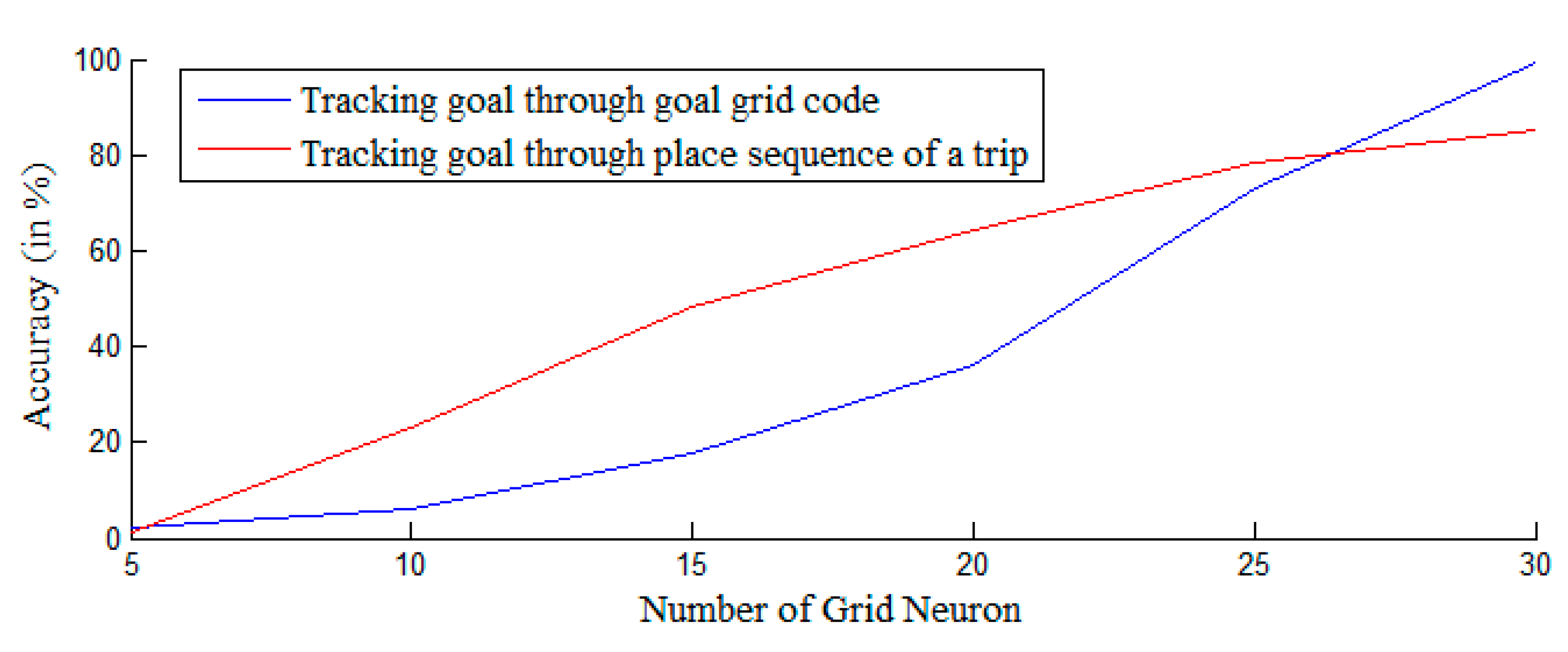
5.4. Comparison between the Navigation Using Tracking Goal Grid Code and Using the Place Sequence (Trip)

The difference between both navigational approaches is the time complexity and the accuracy because in the navigation through tracking of distant place grid code, only a single time direction, and the distance is required to calculate. However, in the case of obstacles, an agent may have to change its current path resulting in recalculating the distance and direction from the changed path. In contrast to grid code, in the case of a trip, this corresponds to each recalled place neuron of the learned trip, the direction, and the distance is required to calculate to move forward, which makes it time inefficient in processing.

As far as accuracy is concerned, if the target grid code is far, then in case of tracking using goal grid code will be lower compared to using a learned trip for navigation. The results of the accuracy of both cases are shown in Figure 24, where the vertical axis representing the goal-tracking accuracy, and the horizontal axis represents the number of grid neurons used.

The accuracy for tracking the goal location through the goal grid code is observed to be highly error-prone at a smaller number of grid neurons, due to the possibility of ambiguity in a large conjunctive grid pattern from a current to a goal location, but the accuracy has increased almost exponentially on increasing the number of grid neurons. The accuracy for the tracking using place sequence learner is observed to be less error-prone compared to the tracking through goal grid code. The reason behind this is the less ambiguity between the current and the nearby place grid code in comparison to the current and the goal grid code.

5.5. Accuracy Results on Different Grid Spacings and Size of the Activation Field

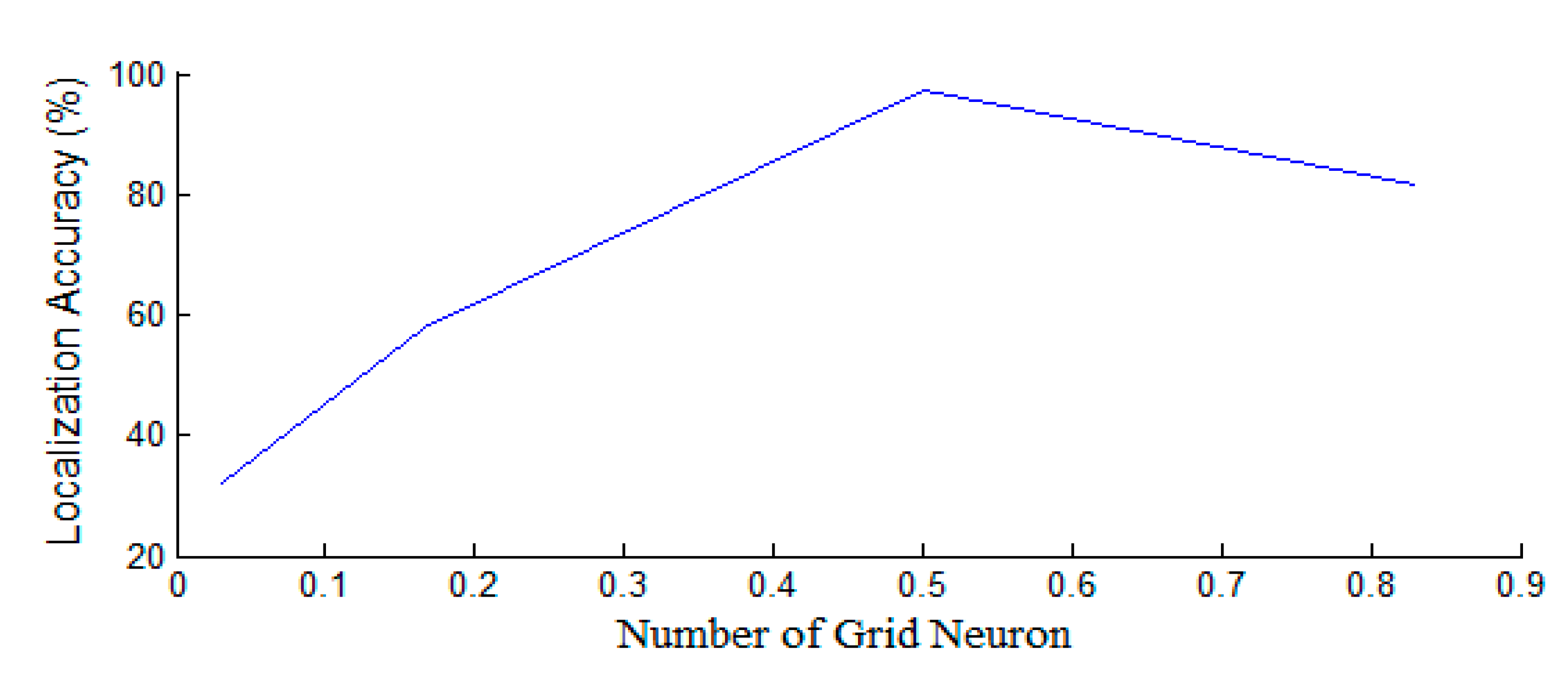
The larger grid spacing grid neurons are those that fire from 2–5 sites in an environment. The grid neuron fires at more than five sites are considered as smaller grid spacing grid neurons. We checked different numbers of smaller and larger grid neurons that are defined as a value, which is a ratio of the number of larger grid spacing grid neurons to the total number of grid neurons. The results for the localization accuracy with respect to the ratio value are shown in Figure 25. The figure has shown poor accuracy at lower ratio value. The poor accuracy is observed due to higher ambiguity in the smaller activation field size grid neuron. In a small activation region, the firing pattern repeats several times in an environment, so it fails to predict the correct sub-area in the environment. On a higher ratio value, the accuracy has reached to its optimum level. The reason behind the optimal accuracy is the correct prediction of the sub-area by the larger grid spacing neurons and the correct location in the sub-area by the smaller grid spacing grid neurons. On the further increase of the ratio value, the accuracy has decreased from the optimal level but not much compared to the lower ratio value. The reason behind this phenomenon is the large grid spacing grid neurons. The large grid spacing neuron predicts the correct sub-area but fails to locate the correct location in a sub-area. Finding the correct location in a sub-area is the task of smaller grid spacing neurons.

5.6. Localization Accuracy in Ambiguous Field

With reference to the previous section, the results for localization error in an unambiguous environment does not require the sequence of touches or further exploration in the environment to localize itself. Furthermore, similar stimuli are present at multiple locations in an ambiguous environment, which confuses the agent to choose a single one in multiple predictions. Therefore the agent must integrate its current path with several previous forecasts until the agent predicts only one location.

The proposed model has outperformed the RatSLAM [17], as depicted in Figure 26, where there were compared in two ambiguous environments. In the first ambiguous environment, on the first sensory input, the model has recalled two different places. That is why the model is confused in the very first decision, and it has chosen randomly one from the two. It results in a poor success rate of around 0.5 in the first decision. However, as it missed the reward due to the first wrong decision, the model has resolved the confusion, and one true place is activated. Thereafter, the only active correct place neuron will activate the correct neuron on path integration so the agent will only make the right decision. On the other hand, the second environment, which is highly ambiguous despite the fact that the model has resolved the confusion using the trip sequence learner (it is an episodic memory). It can store the grid code of the places along with the event activities, which helps in recalling the decisions. Even in the second environment, the first decision is filled with ambiguity, but later the agent resolves the ambiguity using the location sequence learner so that further decisions are all correct.

5.7. Space and Time Complexity

The proposed mechanism has modeled a grid neuron that acts like a bulb whose light intensity increases and decreases in 2D space as per the hexagonal grid sites exactly like grid neurons. At the same time, the other models like RatSLAM [17] have modeled grid neuron as a cell which is spatially placed in a hexagonal pattern in a two-dimensional space. In this view, these multiple hexagonal grids are used to learn places using a Mexican hat function. Since each cell covers a small space of the environment; therefore, their numbers depend on the size of the environment and makes them highly space inefficient. Whereas, in the proposed mechanism, a single grid neuron can generate a hexagonal pattern for any size environment, here, multiple grid neurons are used to increase the accuracy of localization, where the number is dependent on the accuracy level of localization, not on the environment size.

Since the number of grid neurons is much less compared to the RatSLAM, therefore the proposed mechanism is highly space-efficient. The time complexity of the grid models directly dependent on the number of grid cells, which are much less in our case. That is why the proposed model would be superior in the time complexity as well. In RatSLAM, for a task of localization in an environment of size 10 × 10 m² the model has required 36 layers of hexagonal grids with 0.25 × 0.25 area for each grid cells. Thus the total number of grid cells in RatSLAM will be 57,600 [17]. Therefore correspond to each place in RatSLAM, activation values of 57,600 grid cells are required to be stored, whereas in the proposed model:

‘n’ is the number of grid neurons

n × (n − 1)/2 distance values,

n—activation value

n—quadrant angle of each grid neuron

In this view, n = (n + 5)/2, for n = 29 (at which the highest accuracy has been achieved), the total number of parameters stored will be 493, corresponding to a place neuron.

6. Conclusions and Future Work

Computational modeling of the grid and the place neuron’s interaction system has given rise to a unique quadrant and interference pattern learning model to mimic the functionality of the grid and the place neuron, respectively. The model is advantageous over the other grid neuron models as it provides the unique functionality of body parts movement tracking to use in several spatial cognitive tasks in addition to navigation. The model is deployed in a virtual agent to work in a 2D virtual environment, and further behavior of the agent is analyzed. The analysis shows that the proposed model is significantly associated with all biological findings and theories related to the grid and the place neuron. Moreover, it seems that activation patterns observed from the quadrant model and the interference model are similar to the activation patterns of a biological grid neuron and place neuron. Computational modeling has uncovered many unseen challenges, like learning an unambiguous grid code to localize with higher accuracy. As the localization accuracy of 92.27% is reported using the proposed mechanism, this shows the applicability of the proposed mechanism in several real-world problems related to spatial semantics.

The human brain can localize body parts on a 3D object that shows a biological grid neuron that can divide any object or environment into a 3D regular hexagonal grid. The proposed quadrant model can only work in a 2D environment, which limits the applicability of the model. However, in the future, the number of quadrants in the quadrant model can be increased from four to eight, so that the model can generate 3D grid patterns in a 3D environment.

References

1. Chatila, R.; Laumond, J.-P. Position referencing and consistent world modeling for mobile robots. In Proceedings of the 1985 IEEE International Conference on Robotics and Automation, St. Louis, MO, USA, 25–28 March 1985; Volume 2, pp. 138–145. [Google Scholar]
2. Durrant-Whyte, H.; Bailey, T. Simultaneous localization and mapping: Part I. IEEE Robot. Autom. Mag. 2006, 13, 99–110. [Google Scholar] [CrossRef] [Green Version]
3. Rodríguez, F.J.S.; Moreno, V.; Curto, B.; Álves, R. Semantic Localization System for Robots at Large Indoor Environments Based on Environmental Stimuli. Sensors 2020, 20, 2116. [Google Scholar] [CrossRef] [Green Version]
4. Mcelhoe, B.A. An Assessment of the Navigation and Course Corrections for a Manned Flyby of Mars or Venus. IEEE Trans. Aerosp. Electron. Syst. 1966, 2, 613–623. [Google Scholar] [CrossRef]
5. Jauffret, A.; Cuperlier, N.; Gaussier, P. From grid cells and visual place cells to multimodal place cell: A new robotic architecture. Front. Neurorobot. 2015, 9, 1. [Google Scholar] [CrossRef]
6. O’Keefe, J.; Burgess, N.; Donnett, J.G.; Jeffery, K.J.; Maguire, E.A. Place cells, navigational accuracy, and the human hippocampus. Philos. Trans. R. Soc. Lond. Ser. B Biol. Sci. 1998, 353, 1333–1340. [Google Scholar] [CrossRef] [PubMed]
7. O’Keefe, J.; Dostrovsky, J. The hippocampus as a spatial map. Preliminary evidence from unit activity in the freely-moving rat. Brain Res. 1971, 34, 171–175. [Google Scholar] [CrossRef]
8. Hafting, T.; Fyhn, M.; Molden, S.; Moser, E.I.; Moser, E.I. Microstructure of a spatial map in the entorhinal cortex. Nature 2005, 436, 801–806. [Google Scholar] [CrossRef]
9. Fyhn, M.; Hafting, T.; Witter, M.P.; Moser, E.I.; Moser, M.-B. Grid cells in mice. Hippocampus 2008, 18, 1230–1238. [Google Scholar] [CrossRef]
10. Yartsev, M.M.; Witter, M.P.; Ulanovsky, N. Grid cells without theta oscillations in the entorhinal cortex of bats. Nature 2011, 479, 103–107. [Google Scholar] [CrossRef]
11. Killian, N.J.; Jutras, M.J.; Buffalo, E.A. A map of visual space in the primate entorhinal cortex. Nature 2012, 491, 761–764. [Google Scholar] [CrossRef]
12. Jacobs, J.; Weidemann, C.T.; Miller, J.F.; Solway, A.; Burke, J.F.; Wei, X.-X.; Suthana, N.; Sperling, M.R.; Sharan, A.D.; Fried, I.; et al. Direct recordings of grid-like neuronal activity in human spatial navigation. Nat. Neurosci. 2013, 16, 1188–1190. [Google Scholar] [CrossRef] [PubMed] [Green Version]
13. Doeller, C.F.; Barry, C.; Burgess, N. Evidence for grid cells in a human memory network. Nature 2010, 463, 657–661. [Google Scholar] [CrossRef] [PubMed]
14. Moser, E.I.; Kropff, E.; Moser, M.B. Place cells, grid cells, and the brain’s spatial representation system. Annu. Rev. Neurosci. 2008, 31, 69–89. [Google Scholar] [CrossRef] [PubMed] [Green Version]
15. Bush, D.; Barry, C.; Burgess, N. What do grid cells contribute to place cell firing? Trends Neurosci. 2014, 37, 136–145. [Google Scholar] [CrossRef] [PubMed] [Green Version]
16. McNaughton, B.L.; Battaglia, F.P.; Jensen, O.; Moser, E.I.; Moser, M.-B. Path integration and the neural basis of the’cognitivemap. Nat. Rev. Neurosci. 2006, 7, 663–678. [Google Scholar] [CrossRef] [PubMed]
17. Milford, M.; Wiles, J.; Wyeth, G.F. Solving Navigational Uncertainty Using Grid Cells on Robots. PLoS Comput. Biol. 2010, 6, e1000995. [Google Scholar] [CrossRef] [Green Version]
18. Burgess, N.; Barry, C.; O’Keefe, J. An oscillatory interference model of grid cell firing. Hippocampus 2007, 17, 801–812. [Google Scholar] [CrossRef] [PubMed] [Green Version]
19. Bush, D.; Burgess, N. A hybrid oscillatory interference/continuous attractor network model of grid cell firing. J. Neurosci. 2014, 34, 5065–5079. [Google Scholar] [CrossRef] [PubMed] [Green Version]
20. Savelli, F.; Knierim, J.J. Origin and role of path integration in the cognitive representations of the hippocampus: Computational insights into open questions. J. Exp. Biol. 2019, 222 (Suppl. 1). [Google Scholar] [CrossRef] [Green Version]
21. O’Keefe, J.; Lynn, N. The Hippocampus as a Cognitive Map; Clarendon Press: Oxford, UK, 1978. [Google Scholar]
22. Leutgeb, S.; Leutgeb, J.K.; Barnes, C.A.; Moser, E.I.; McNaughton, B.L.; Moser, M.B. Independent Codes for Spatial and Episodic Memory in Hippocampal Neuronal Ensembles. Science 2005, 309, 619–623. [Google Scholar] [CrossRef] [PubMed] [Green Version]
23. Rolls, E.T.; Stringer, S.M.; Trappenberg, T.P. A unified model of spatial and episodic memory. Proc. R. Soc. Lond. Ser. B Biol. Sci. 2002, 269, 1087–1093. [Google Scholar] [CrossRef] [PubMed] [Green Version]
24. Shrivastava, R.; Tripathi, S. Computational Model of Episodic Memory Formation, Recalling, and Forgetting. In Proceedings of the International Conference on Recent Advancement on Computer and Communication; Springer: Singapore, 2018; Volume 34, pp. 395–403. [Google Scholar]
25. Kolisetty, V.; Rajput, D. A Review on the Significance of Machine Learning for Data Analysis in Big Data. Jordanian J. Comput. Inf. Technol. 2019, 6. [Google Scholar] [CrossRef]
26. Reddy, G.T.; Reddy, M.P.K.; Lakshmanna, K.; Kaluri, R.; Rajput, D.S.; Srivastava, G.; Baker, T. Analysis of Dimensionality Reduction Techniques on Big Data. IEEE Access 2020, 8, 54776–54788. [Google Scholar] [CrossRef]
27. Tiwari, V.; Thakur, R.S. Pattern Warehouse: Context Based Modeling and Quality Issues. Proc. Natl. Acad. Sci. India Sect. A Phys. Sci. 2016, 86, 417–431. [Google Scholar] [CrossRef]
28. Tiwari, V.; Thakur, R.S. Contextual snowflake modelling for pattern warehouse logical design. Sadhana 2015, 40, 15–33. [Google Scholar] [CrossRef]
29. Iwendi, C.; AlQarni, M.A.; Anajemba, J.H.; Alfakeeh, A.S.; Zhang, Z.; Bashir, A.K. Robust Navigational Control of a Two-Wheeled Self-Balancing Robot in a Sensed Environment. IEEE Access 2019, 7, 82337–82348. [Google Scholar] [CrossRef]
30. Patel, H.; Rajput, D.S.; Reddy, G.T.; Iwendi, C.; Bashir, A.K.; Jo, O. A review on classification of imbalanced data for wireless sensor networks. Int. J. Distrib. Sens. Netw. 2020, 16. [Google Scholar] [CrossRef]
31. Deepa, N.; Prabadevi, B.; Maddikunta, P.K.R.; Gadekallu, T.R.; Baker, T.; Khan, M.A.; Tariq, U. An AI-based intelligent system for healthcare analysis using Ridge-Adaline Stochastic Gradient Descent Classifier. J. Supercomput. 2020. [Google Scholar] [CrossRef]
32. Godard, C.; Mac Aodha, O.; Brostow, G.J. Unsupervised Monocular Depth Estimation with Left-Right Consistency. In Proceedings of the 2017 IEEE Conference on Computer Vision and Pattern Recognition (CVPR), Honolulu, HI, USA, 21–26 July 2017; pp. 6602–6611. [Google Scholar]
33. Poluru, R.K.; Reddy, M.P.K.; Kaluri, R.; Lakshmanna, K.; Reddy, G.T. Agribot. In Advances in Computer and Electrical Engineering; IGI Global: Hershey, PA, USA, 2020; pp. 151–157. [Google Scholar]
34. Tang, Q.; Yang, K.; Zhou, D.; Luo, Y.-S.; Yu, F. A Real-Time Dynamic Pricing Algorithm for Smart Grid With Unstable Energy Providers and Malicious Users. IEEE Internet Things J. 2015, 3, 554–562. [Google Scholar] [CrossRef]
35. He, S.; Zeng, W.; Xie, K.; Yang, H.; Lai, M.; Su, X. PPNC: Privacy Preserving Scheme for Random Linear Network Coding in Smart Grid. KSII Trans. Internet Inf. Syst. 2017, 11, 1510–1532. [Google Scholar] [CrossRef]
36. Xia, Z.; Tan, J.; Wang, J.; Zhu, R.; Xiao, H.; Sangaiah, A.K. Research on Fair Trading Mechanism of Surplus Power Based on Blockchain. J. UCS 2019, 25, 1240–1260. [Google Scholar]
37. Tu, Y.; Lin, Y.; Wang, J. Semi-supervised Learning with Generative Adversarial Networks on Digital Signal Mod-ulation Classification. Comput. Mater. Contin. 2018, 55, 243–254. [Google Scholar]
38. Liu, M.; Cheng, L.; Qian, K.; Wang, J.; Wang, J.; Liu, Y. Indoor acoustic localization: A survey. Hum. Cent. Comput. Inf. Sci. 2020, 10, 2. [Google Scholar] [CrossRef]
39. Chen, Y.; Xiong, J.; Xu, W.; Zuo, J. A novel online incremental and decremental learning algorithm based on variable support vector machine. Clust. Comput. 2018, 22, 7435–7445. [Google Scholar] [CrossRef]
40. Li, H.; Li, W.; Zhang, S.; Wang, H.; Pan, Y.; Wang, J. Page-sharing-based virtual machine packing with multi-resource constraints to reduce network traffic in migration for clouds. Future Gener. Comput. Syst. 2019, 96, 462–471. [Google Scholar] [CrossRef]
41. Singh, S.; Ra, I.-H.; Meng, W.; Kaur, M.; Cho, G.H. SH-BlockCC: A secure and efficient Internet of things smart home architecture based on cloud computing and blockchain technology. Int. J. Distrib. Sens. Netw. 2019, 15, 1550147719844159. [Google Scholar] [CrossRef]
42. Zhang, D.; Yin, T.; Yang, G.; Xia, M.; Li, L.; Sun, X. Detecting image seam carving with low scaling ratio using multi-scale spatial and spectral entropies. J. Vis. Commun. Image Represent. 2017, 48, 281–291. [Google Scholar] [CrossRef]
Figure 1. Grid neuron activation.
Applsci 10 05147 g001
Figure 2. Grid activation patterns of different spacing and orientations.
Applsci 10 05147 g002
Figure 3. The connectivity of place and grid neuron.
Applsci 10 05147 g003
Figure 4. Localization using overlapped grid patterns.
Applsci 10 05147 g004
Figure 5. Ambiguity in grid code.
Applsci 10 05147 g005
Figure 6. Agent’s movement.
Applsci 10 05147 g006
Figure 7. Geometry of quadrants.
Applsci 10 05147 g007
Figure 8. Coordinate calculation.
Applsci 10 05147 g008
Figure 9. The geometry of hexagonal grid points.
Applsci 10 05147 g009
Figure 10. Cognitive mapping of sensory information.
Applsci 10 05147 g010
Figure 11. Grid code learning.
Applsci 10 05147 g011
Figure 12. Interference of grid rings.
Applsci 10 05147 g012
Figure 13. The procedure of sensory information prediction.
Applsci 10 05147 g013
Figure 14. Place sequence learner.
Applsci 10 05147 g014
Figure 15. Object representation.
Applsci 10 05147 g015
Figure 16. Depth image conversion: (a) original image, (b) depth image.
Applsci 10 05147 g016
Figure 17. Illustration of agent navigation.
Applsci 10 05147 g017
Figure 18. Output grid patterns of the quadrant model: (a) grid spacing of 15 units taken with the grid ring radius of 3 units; (b) grid spacing of 35 units with the grid ring radius of 10 units; (c) spacing of 25 units, radius 3 units and orientation of 30 degrees; (d) spacing of 25 units, grid ring radius is of 3 units and orientation of 10 degrees; (e) spacing of 55 units, and radius of 10 units; (f) Interference of two different grid patterns.
Applsci 10 05147 g018
Figure 19. Place selective activation patterns of two individual place cells inside and outside the place field.
Applsci 10 05147 g019
Figure 20. Grid code.
Applsci 10 05147 g020
Figure 21. Object recognition.
Applsci 10 05147 g021
Figure 22. Error in self-localization.
Applsci 10 05147 g022
Figure 23. Trip strength dynamics.
Applsci 10 05147 g023
Figure 24. Performance comparison on localization.
Applsci 10 05147 g024
Figure 25. Effect of grid neuron population on localization.
Applsci 10 05147 g025
Figure 26. Localization in an ambiguous environment.
Applsci 10 05147 g026