Article

A Hybrid Deep Learning Framework for Unsupervised Anomaly Detection in Multivariate Spatio-Temporal Data

by
Yıldız Karadayı
1,*,
Mehmet N. Aydin
2 and
A. Selçuk Öğrenci
3
1
Computer Engineering, Kadir Has University, 34083 İstanbul, Turkey
2
Management Information Systems, Kadir Has University, 34083 İstanbul, Turkey
3
Electrical-Electronics Engineering, Kadir Has University, 34083 İstanbul, Turkey
*
Author to whom correspondence should be addressed.
Appl. Sci. 2020, 10(15), 5191; https://doi.org/10.3390/app10155191
Submission received: 23 June 2020 / Revised: 21 July 2020 / Accepted: 23 July 2020 / Published: 28 July 2020
(This article belongs to the Section Computing and Artificial Intelligence)

Abstract

:
Multivariate time-series data with a contextual spatial attribute have extensive use for finding anomalous patterns in a wide variety of application domains such as earth science, hurricane tracking, fraud, and disease outbreak detection. In most settings, spatial context is often expressed in terms of ZIP code or region coordinates such as latitude and longitude. However, traditional anomaly detection techniques cannot handle more than one contextual attribute in a unified way. In this paper, a new hybrid approach based on deep learning is proposed to solve the anomaly detection problem in multivariate spatio-temporal dataset. It works under the assumption that no prior knowledge about the dataset and anomalies are available. The architecture of the proposed hybrid framework is based on an autoencoder scheme, and it is more efficient in extracting features from the spatio-temporal multivariate datasets compared to the traditional spatio-temporal anomaly detection techniques. We conducted extensive experiments using buoy data of 2005 from National Data Buoy Center and Hurricane Katrina as ground truth. Experiments demonstrate that the proposed model achieves more than 10% improvement in accuracy over the methods used in the comparison where our model jointly processes the spatial and temporal dimensions of the contextual data to extract features for anomaly detection.

1. Introduction

An anomaly is an observation whose properties are significantly different from the majority of other observations under consideration which are called the normal data. Anomaly detection refers to the problem of finding these observations that do not adhere to expected or normal behavior. A spatio-temporal outlier (ST-Outlier) is an object with behavioral (non-contextual) attributes that are notably different from other objects in the neighborhood which is defined by its contextual (spatial and temporal) attributes [1]. Spatio-temporal data have become extremely common in many application domains because of the advancement of the hardware technology for data collection and generation. Collecting data from various spatial locations and at regular time intervals are very important for some problem settings. In such settings, detection of spatio-temporal outliers can lead to the discovery of interesting and generally unexpected patterns such as local instability [2]. Some examples of such spatio-temporal datasets are as follows: meteorological data, traffic data, earth science, and disease outbreak data. Events that generate spatio-temporal data are evolving events, such as hurricanes and disease outbreaks, and both spatial and temporal continuity are important in modelling such events [3].
For a problem domain, obtaining the labelled training data for all types of anomalies is often too expensive if not impossible [4]. This highlights the need for unsupervised techniques to find spatio-temporal anomalies. Moreover, spatio-temporal datasets are generally multivariate and have many contextual structures in them (spatial and temporal regularities) which makes them particularly difficult for labelling and well suited for unsupervised learning models. In the unsupervised scenarios, the type of anomalies and the ratio of anomalous events within the given dataset are generally not known. In such scenarios, we need to model the normal behavior of the underlying system in the presence of anomalies which pose extra difficulty.
In the past few years, some density- and clustering-based unsupervised spatio-temporal anomaly detection algorithms have been developed. The most prominent ones are ST-Outlier detection algorithm [5] and ST-BDBCAN [6] methods which are basically an extension of DBSCAN [7], a density-based spatial clustering algorithm. LDBSCAN [8], a locality-based outlier detection algorithm, is the merge of both DBSCAN and Local Outlier Factor (LOF) [9]. IsolationForest [10,11] is a powerful approach for anomaly detection in multivariate data without relying on any distance or density measure. In particular, it is an unsupervised, tree-based ensemble method that applies the novel concept of isolation to anomaly detection. It detects anomalies based on a fundamentally different model-based approach: an anomalous point is isolated via recursive partitioning by randomly selecting a feature and then randomly selecting a split value for the selected feature. The output is the anomaly score for each data point. Although it establishes a powerful multivariate non-parametric approach, it works on continuous-valued data only. Despite the inherent unsupervised setting, they may still not detect anomalies effectively due to the following reasons:
  • In multivariate time series data, strong temporal dependency exists between time steps. Due to this reason, distance-/clustering-based methods, may not perform well since they cannot capture temporal dependencies properly across different time steps.
  • On the other hand, for the case of high-dimensional data, even the data locality may be ill-defined because of data sparsity [3].
  • Despite the effectiveness of IsolationForest technique, it isolates data points based on one random feature at a time which may not represent spatial and temporal dependencies between data points properly in the spatio-temporal dataset.
  • The definition of distance between data points in multivariate spatio-temporal data with mixed attributes is often challenging. This difficulty may have an adverse effect on outlier detection performance of distance-based clustering algorithms.
To address these challenges, we propose a hybrid deep autoencoder framework. It is composed of a multi-channel convolutional neural network (CNN) and Long Short-Term Memory (LSTM) network, named as MC-CNN-LSTM. The architecture of the proposed hybrid framework is based on the autoencoder scheme which has the greater power in representing arbitrary data distributions for anomaly detection than commonly used alternatives such as PCA or matrix factorization [12]. The multi-channel CNN network is deployed on the encoder side for learning spatial structures of each spatio-temporal multivariate data frame, and LSTM network is deployed on the decoder side for learning temporal patterns from the encoded spatial structures. It is designed to solve the unsupervised anomaly detection problem in non-image multivariate spatio-temporal data. Our major contributions in this paper can be summarized as follows:
  • In the aforementioned neighborhood methods, the biggest challenge is to combine the contextual attributes in a meaningful way. In the proposed approach, spatial and temporal contexts are handled by different deep learning components as these contextual variables refer to different types of dependencies.
  • All distance-/clustering-based algorithms are proximity-based algorithms and dependent on some notion of distance. Many distance functions used for proximity quantification (such as Euclidean and Manhattan) are not meaningful for all datatypes.
  • The proposed hybrid framework is designed to be trained in a truly unsupervised fashion without any labels indicating normal or abnormal data. The architecture is robust enough to learn the underlying dynamics even if the training dataset contains noise and anomalies.
  • In the proposed hybrid architecture, CNN and LSTM layers are combined into one unified framework that is jointly trained. Unlike proximity-based methods, the framework can be easily implemented on data with mixed-type attributes and scales well to multivariate datasets with high number of features.
We compared the proposed model with the state-of-the-art spatial and spatio-temporal anomaly detection algorithms: ST-Outlier detection algorithm [5], ST-BDBCAN [6], LDBSCAN [8], LOF [9], and to a powerful model-based anomaly detection method, IsolationForest [10]. We conducted extensive experiments using the year 2005 Gulf of Mexico (West) buoy dataset from National Data Buoy Center (https://www.ndbc.noaa.gov/) and Hurricane Katrina best track path data [13] as ground truth for the experiments. Our results demonstrate that the proposed deep learning framework achieves superior results by achieving at least 10% improvement in accuracy over the methods used in comparison.
The remainder of this paper is organized as follows. Section 2 provides an overview of related work in the literature. Section 3 gives theoretical background on autoencoders, autoencoder based anomaly detection, CNN and LSTM networks. Section 4 explains methodology, spatio-temporal data pre-processing and the proposed hybrid deep learning framework. Section 5 gives detailed information on experimental setup, Hurricane Katrina dataset and results of the experiments. Section 6 discusses the results, summarizes contributions and gives the future research directions.

2. Related Work

The task of detecting outliers or anomalous events in data has been studied extensively in the context of time series and spatial data separately. Outlier detection studies for time-series data find outliers considering only the temporal context [14,15]. For data with spatial context, several context-based anomaly detection techniques have been proposed [16,17,18,19,20]. Spatio-temporal outlier detection methods are significantly more challenging because of the additional difficulty of jointly modeling the spatial and temporal continuity in the dataset [2,3].
Birant and Kut [5] propose a spatio-temporal outlier detection algorithm using a modified version of DBSCAN. It is a neighborhood-based approach which first defines spatial outliers based on spatial neighborhood, then checks the temporal context of spatial outliers using their temporal neighbors. However, their algorithm does not generate a score for data points. Cheng and Li [2] propose a four-step sequential approach to identify spatio-temporal outliers using classification, aggregation, comparison, and verification. Gupta et al. [20] introduce the notion of context-aware anomaly detection by integrating the system logs and time series measurement data in distributed systems. They propose a two-stage clustering methodology using a principle component analysis (PCA) [21] based method and K-Means [22] algorithm to extract context and metric patterns.
The methods mentioned above have something in common: They do not use the spatial and temporal components jointly to detect anomalies. They first find spatial outliers using spatial context. Then, they use temporal context to define temporal neighborhood of spatial outliers to detect if they are temporal outliers too. They all use either a modified version of DBSCAN [7], which is a spatial clustering-based outlier detection algorithm, or LOF [9], which is a locality-based outlier detection algorithm, to find neighborhoods. The main challenge with distance-based methods is that they are computationally too expensive for large multivariate datasets.
The idea of isolation and IsolationForest algorithm have been successfully applied in anomaly detection and rare class classification problems in different data domains. Alanso-Sarria et al. [23] apply IsolationForest analysis into the landcover image dataset to measure the representativeness of training areas in the image. Chen et al. [24] propose an isolation-based online anomalous trajectory detection system to detect abnormal or malicious events using trajectories obtained from Global Position System (GPS)-enabled taxis. Stripling et al. [25] propose an IsolationForest based conditional anomaly detection approach for fraud detection.
Besides traditional distance- and isolation-based methods, deep learning-based anomaly detection approaches have recently gained a lot of attention. LSTM networks have been used for anomaly detection on time series data as it achieves better generalization capability than traditional methods. A LSTM network-based Encoder–Decoder scheme for anomaly detection was recently proposed where the model learns to reconstruct ‘normal’ time series data and uses reconstruction error to detect anomalies [26]. A recent deep learning anomaly detection approach combining a convolutional neural network (CNN), LSTM, and deep neural network (DNN) were designed to detect traffic anomalies in web servers [27], where they used fully labeled dataset for supervised learning and solved a univariate time series classification problem. Another deep learning framework combining a convolutional encoder, attention-based convolutional LSTM network, and convolutional decoder for detecting spatio-temporal anomalies for multivariate time series data was proposed [28]. In addition to network complexity, their approach requires the calculation of multiscale system signature and residual signature matrices to perform anomaly detection thereby increasing the overall complexity.
Christiansen et al. [29] propose convolutional neural network (CNN)-based anomaly detection system to detect obstacles in an agriculture field. Their anomaly detection framework uses features extracted by a CNN detector. Oh and Yun [30] propose an autoencoder-based approach to detect abnormal operations of a complex machine using operational sound. They adopt a general convolutional autoencoder architecture and use residual errors to detect anomalies. Munir at el. [31] propose a novel approach for anomaly detection in streaming sensors data which takes advantage of both statistical and deep learning-based techniques. They use statistical ARIMA model and a convolutional neural network (CNN) model to forecast the next timestamp in a given time-series. The forecasted value is further passed to an anomaly detector module that marks a data point as normal or anomalous based on the distance between the predicted value and the actual value.
Despite the effectiveness of those abovementioned deep learning approaches, they are either supervised or semi-supervised models which need labelled normal or abnormal data for training. The proposed hybrid framework is designed to be trained in a truly unsupervised fashion without any labels indicating normal or abnormal data. The architecture is robust enough to learn the underlying dynamics even if the training dataset contains noise and anomalies. The main distinction between other deep learning-based methods and the proposed approach is that they perform on either univariate or multivariate time series data, and none of them is actually designed for spatio-temporal multivariate datasets with both spatial and temporal contextual attributes.

3. Background

3.1. Autoencoders

Autoencoders are commonly used for dimensionality reduction of multidimensional data as a powerful non-linear alternative to PCA or matrix factorization [32,33,34]. If a linear activation function is used, the autoencoder becomes virtually identical to a simple linear regression model or PCA/matrix factorization model. When a nonlinear activation function is used, such as rectified linear unit (ReLU) or a sigmoid function, the autoencoder goes beyond the PCA, capturing multi-modal aspects of the input distribution [12,35]. It is shown that carefully designed autoencoders with tuned hyperparameters outperform PCA or K-Means methods in dimension reduction and characterizing data distribution [36,37]. They are also more efficient in detecting subtle anomalies than linear PCAs and in computation cost than kernel PCAs [32,38].
A traditional autoencoder is a feed-forward multi-layer neural network which is trained to copy its input into the output. To prevent identity mapping, deep autoencoders are built with low dimensional hidden layers by creating non-linear representation of input data [32]. An autoencoder is trained to encode the input x into some latent representation z so that the input can be reconstructed from that lower dimensional representation. An autoencoder is trained by unsupervised learning to learn how to build its original input with a minimum reconstruction error. Figure 1 depicts a typical autoencoder network structure with one hidden layer, being composed of two parts: an encoder and decoder. Deep autoencoders learn a non-linear mapping from the input to the output through multiple encoding and decoding steps. An autoencoder takes an input vector x R d , and first maps it to a latent representation z R d through the mapping:
z = f θ ( x ) = W x + b
where the function f θ represents the encoding steps and parameterized by θ = { W , b } . W is a d × d   weight matrix and b is a bias vector. The lower dimensional latent representation of the input is then mapped back to a reconstructed vector x R d in the input space
x = g θ ( z ) = W z + b
where the function g θ represents the decoding steps and parameterized by θ = { W , b } . The autoencoders training procedure consists of finding a set of parameters { W ,   b ,   W , b } that make the reconstructed vector x as close as possible to the original input x . The parameters of the autoencoder are optimized by minimizing a loss function that measures the quality of the reconstructions. The loss function of an autoencoder is sum-of-squared differences between the input and the output. Therefore, an autoencoder tries to minimize the following loss function during the training:
L ( x , x ) = x φ i = 1 d x i x i 2 ,
where φ is the training dataset.

3.2. Anomaly Detection with Autoencoders

The main idea behind autoencoder based anomaly detection is to measure how much the reconstructed data deviates from the original data. An autoencoder has an unsupervised learning objective whose primary task is to copy the input to the output [39]. Therefore, an autoencoder is trained to reconstruct data by minimizing this objective function, or loss function. For anomaly detection, reconstruction error is used as the anomaly score. Data points which generate high reconstruction errors can be categorized as anomalous data points based on a threshold value. When autoencoders are used for anomaly detection, they are trained using semi-supervised learning. In this scenario, only normal data instances are used in training process. The training dataset should be cleaned from anomalous data points and outliers as much as possible for a successful model generation. Therefore, for the anomaly detection model to be successful, it is critical to design a pre-processing phase that can filter out or correct such noise from the data when possible. This can be achieved using a variety of unsupervised domain-specific methods, such as statistical and distance-based methods. For example, in the context of time series data, autoregressive models, in the context of spatial data, distance- and density-based models can be used for noise removal. Techniques such as Principle Component Analysis (PCA) and Singular Value Decomposition (SVD) methods can also be used in order to improve the representation quality of data and remove discordant data points [1,3]. After the training process, the autoencoder will generally reconstruct normal data with very small reconstruction error. As the autoencoder has not encountered with the abnormal data during the training, it will fail to reconstruct them and generate high reconstruction errors which can be used as anomaly score.
There are some practical issues in using autoencoders with contaminated training data (dataset with normal and anomalous data points). Since anomalies are treated as normal data points during the training phase, there will be inevitably more errors in the model compared to training with only normal data points. If we try to overcome these errors by tuning the network with more layers and neurons, we may face the problem of overfitting which is the significant problem in the case of deep neural networks. A sufficiently complex deep autoencoder may even learn how to represent each anomaly with sufficient training by generating low reconstruction errors which would be a problem in anomaly detection [3].

3.3. Convolutional Neural Networks (CNNs)

Fully convolutional networks have shown compelling quality and efficiency for image classification and segmentation. It has been shown that a fully convolutional network, which is trained end to end, pixel to pixel, given the category-wise semantic segmentation annotation, exceeds the state of the art without further creating hand-crafted features [40,41].
The layers of a convolutional neural network are arranged to represent spatial information within data in a grid structure. These spatial relationships are inherited from one layer to the next creating representative features based on a small local spatial region in the previous layer. This spatial transformation is achieved by three types of layers which are commonly present in a convolutional neural network: convolution, pooling, and activation function layers. Each layer in the convolutional network represents a three-dimensional grid structure of size h   ×   w   ×   d , where height ( h ), width ( w ) and depth ( d ), h and w are spatial dimensions, and d refers to the number of channels or the number of feature maps in the hidden layers. In addition to hidden layers, a final set of fully connected layers is often used in an application specific way to generate the desired output [42].
Let x l = [ x i j k l ] be a three-dimensional tensor representing feature maps in the l th layer. The indices i , j , k indicate the positions along the height, width, and depth of the filter maps. The weights of the p th feature map in the l th layer are represented by the three-dimensional tensor as W ( p , l ) = [ w i j k ( p , l ) ] . The transformation from the l th to the ( l + 1 )   st convolutional layer after activation function applied can be written as follows:
y i j p ( l + 1 ) = f ( b p l + r = 1 M s = 1 M k = 1 d l w r s k ( p , l )   x i + r 1 ,   j + s 1 ,   k l )
where f is the activation function, such as t a n h or ReLU, b p l is the bias for the p th feature map, w r s k ( p , l ) represents the parameters of the p th filter, and M is the size of the filter. The convolutional operation is a simple dot product over the entire volume of the filter, which is repeated over spatial dimensions ( i , j ) and filters (indexed by p). d l + 1 is the number of feature maps, or number of channels, in the ( l + 1 )   s t layer, where p     { 1 d l + 1 } .
The pooling operation works on small spatial regions and produces another layer with the same depth. The pooling layers decrease the spatial dimensions of each activation map and effectively reduce the number of parameters and computational complexity of the network. Max pooling and average pooling are the mostly used pooling techniques in CNNs. Max pooling operation with pooling size of R × R returns the maximum of the values in the square region of pool size in each layer. Stride value defines how much the pooling window will move in each spatial dimension, which is another way that convolution can reduce the spatial footprint of the feature maps. Previous studies [43] show that max pooling is superior to average pooling for image classification and it also leads to faster convergence rate and improves generalization performance by preventing overfitting. Hence, the max pooling strategy is applied in convolutional neural network component of the proposed framework.

3.4. Long Short-Term Memory (LSTM) Networks

Autoencoders LSTM network is a type of recurrent neural network (RNN) with controllable memory units that enable the network to learn when to forget previous hidden states and when to update hidden states with new information [44]. They have been proved to be very effective in many long-range sequential modeling applications such as machine translation, speech and action recognition [45,46,47,48]. Generally, LSTM recursively maps the input data at the current time step to a sequence of hidden states, and thus the learning process of LSTM should be in a sequential manner.
LSTM networks address the vanishing gradient problem commonly found in ordinary RNNs by incorporating the concept of gating into their state dynamics. The inputs provided to the LSTM memory unit are fed through gates which are the input, output, and forget gates. At each time step, an LSTM unit updates a hidden state vector h t and a cell state vector c t responsible for controlling state updates and outputs using current input, previous cell state and hidden state values. Specifically, given a sequential data of T timestamps ( x 1 ,   x 2 ,   ,   x T ) , an LSTM memory unit maps the inputs to an output sequence ( y 1 ,   y 2 ,   ,   y T ) by computing the gate functions recursively for each step from t = 1 to t = T with the following equations:
i t = σ ( W x i x t + W h i h t 1 + W c i   c t 1 + b i ) ,
f t = σ ( W x f x t + W h f h t 1 + W c f c t 1 + b f ) ,
o t = σ ( W x o x t + W h o h t 1 + W c o c t + b o )
c t = f t   o   c t 1 + i t o   tan h ( W x c x t + W h c h t 1 + b c ) ,
h t = o t   o   tan h ( c t ) ,
where x t   and h t   are the input and hidden state vectors, the notations i t ,   f t , o t , c t are the activation vectors of the input gate, forget gate, output gate, and memory cell, respectively. W a b is the weight matrix between a and b , and b a is the bias term of a , σ is the sigmoid function. o denotes the element-wise product. The memory cell unit c t is the sum of two terms: the previous memory cell unit modulated by forget gate and a function of the current input and previous hidden state. Input and forget gates can be thought of as knobs that control the learning process: the LSTM learns to selectively forget its previous memory through f t and considers its current input and previous hidden state through i t . The output gate o t learns how much of the current memory cell to transfer to the hidden state. This gated structure seems to enable the LSTM to learn complex and long-term temporal dynamics for contextual data.

4. Methodology

4.1. Spatio-Temporal Data Pre-Processing

A univariate time series is a sequence of data points with timestamps representing contextual dimension. A multivariate time series is a set of univariate time series with the same timestamps. On the other hand, multivariate time series data can be thought as a dataset composed of many univariate time series, which are measured at successive points in time and spaced at uniform time intervals. A spatio-temporal multivariate data point is a multivariate time series observation with a spatial attribute (a contextual attribute) attached to it.
Let X = { x ( n ) } n = 1 N denote a multivariate time series dataset composed of N subsequences of multivariate observations (data points). Each subsequence has the same number of time steps, or window size, which is generated from a long multivariate time series data. Let each subsequence x ( n ) has T time steps, and each observation at time step t, is a d dimensional vector. The dataset X has dimensions of (N, d, T), where x ( n )   d × T . Each sample from multivariate time series dataset can be represented as:
x ( n ) = ( x 11 n x 1 T n x d 1 n x d T n   )
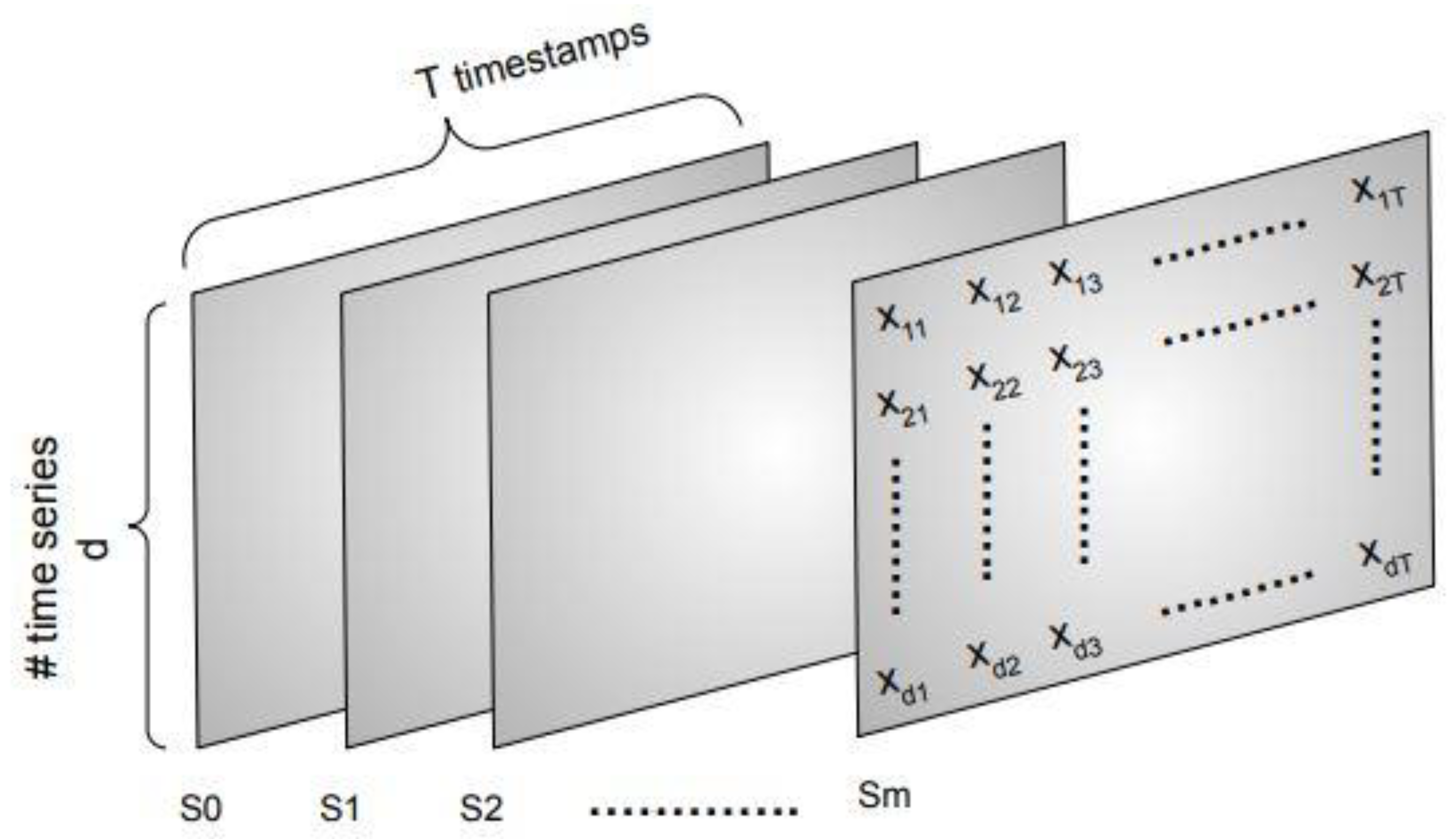
In a spatio-temporal dataset, each multivariate data point x ( n ) comes from a different spatial location, or region, which has different spatial attributes (such as latitude and longitude). Specifically, each multivariate data point has a spatial attribute s ( n ) attached to it. We denote multivariate spatio-temporal dataset as DST = { ( X ( i ) , s ( i ) ) } i = 1 S which contains N ( i ) multivariate data points from S different spatial regions. The multivariate spatio-temporal data matrix X S T can be represented as a three-dimensional matrix, as shown in Figure 2. It is considered as a group of many multivariate subsequences related to multiple spatial regions and representing observations from the same time window with the same timestamps. T , which is called the “input window-size”, represents the number of timestamps in the multivariate subsequence, and d represents the number of observed features (number of univariate time series). m represents the number of spatial neighborhoods to include in the anomaly detection process. The best m can be found empirically for each problem domain. m number of neighboring regions are selected from S different spatial regions by a distance based nearest neighbor algorithm using pairwise spatial distance between regions.

4.2. Anomaly Detection Procedure

The spatio-temporal anomaly detection problem is formulated as detecting anomalous multivariate observations in dataset DST which differentiate significantly from their spatial and temporal neighbors. Given the spatio-temporal three-dimensional data matrix X S T , the goal is to reconstruct the multivariate subsequences from the spatial region S i , which is the region of interest. Anomalous data points have large reconstruction errors because they do not conform to the subspace patterns in the data. Therefore, for the proposed encoder–decoder-based anomaly detection framework, the aggregate error of reconstruction over all d dimensions can be used as the anomaly score. All x i ( n ) multivariate data points, or subsequences, with high reconstruction errors from the spatial region S i are considered to be anomalies.
The anomaly detection process is performed using the reconstruction error as anomaly score. Let x = { x ( 1 ) ,   x ( 2 ) ,   ,   x ( T ) } be a multivariate time series data point from the multivariate time series dataset X , where x     d × T , T is the length of the time series window, and d is the number of features (univariate time series). Each point x ( i ) is a d-dimensional vector of readings for d variables at time instance t i . The root mean squared error (RMSE) is used to calculate the reconstruction error for a given time step t i as given by the following equation:
e ( i ) = 1 d   d   ( x i x ^ i ) 2
where x i is the real value and x ^ i is the reconstructed value at time step t i . The reconstruction error for each time step in the output data is calculated. The result is the aggregated error of output data which has a window size of T . These aggregated errors of data points can be used as anomaly score and high scoring data points are regarded as spatio-temporal anomalies.
The proposed framework uses unlabeled spatio-temporal data points for training. Training data might be contaminated by anomalous data which is the case in most of the real-word scenarios. The multi-channel CNN architecture helps to overcome the problem of overfitting. It processes data which come from m spatial neighborhoods simultaneously and extracts representative features of it. This approach helps to build a model that represents the great majority of data points and not the anomalous points which are rare. Anomalous observations can be thought of as noise and the framework is designed to be robust enough not to learn representation of those points. The framework is trained to reconstruct data by minimizing a loss function (mean squared error) that measures the quality of the reconstructions. Our main hypothesis is that after training, the model is able to reconstruct the input data that conform to expected or normal behavior within the dataset, while it fails to reconstruct anomalous data, since it has not learned any features to represent them.

4.3. Proposed Hybrid Framework

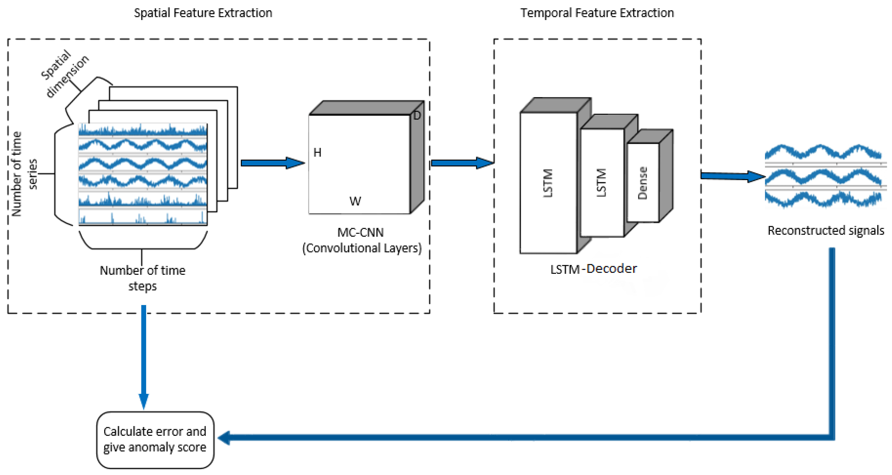
The proposed hybrid framework consists of two major components: a multi-channel convolutional neural network-based encoder (MC-CNN-Encoder) and a Long Short-Term Memory-based decoder (LSTM-Decoder). The framework is connected in a linear structure and trained jointly to minimize the reconstruction error. The CNN layers are an important part of the framework and work as encoder to extract spatial features. The multi-channel structure helps to capture the spatial dependencies in neighboring spatial regions. The reconstruction error of the framework for the given data point is used for anomaly score. Our model design is inspired by the network combining CNN and LSTM into one unified architecture for text prediction problem [49], which shows that LSTM performance can be improved by providing better features. The overall architecture of the framework is illustrated in Figure 3.
The performance of the designed framework depends on various components and training parameters. The number of layers and units in each layer, the number of kernels used in each convolutional layer, dropout ratio and type and size of pooling operators are all important parameters in the anomaly detection process as they can affect the learning performance and speed. They play an important role in extracting more representative features of the training data. To determine the optimal architecture and the best training parameters for the overall network, including the optimum parameters used to preprocess the raw data such as window size and step size, the characteristics of the input data have to be analyzed carefully. In this study, the number of layers and neurons on each layer are selected accordingly to the best empirical performance of grid search on training dataset.

4.3.1. MC-CNN-Encoder

For the spatial encoder component, an effective multi-channel convolutional encoder is proposed. Each channel of the encoder takes multivariate time series data from different spatial neighbors as input. Using the multichannel approach, spatio-temporal features from spatial neighborhood of data points can be extracted. As in image data, multivariate spatio-temporal data are processed by 2D kernels and 2D pooling operations. In contrast to other deep learning approaches which apply CNN on time series data with 1D kernels to extract temporal features [50,51,52], 2D kernels are applied to extract spatial features.
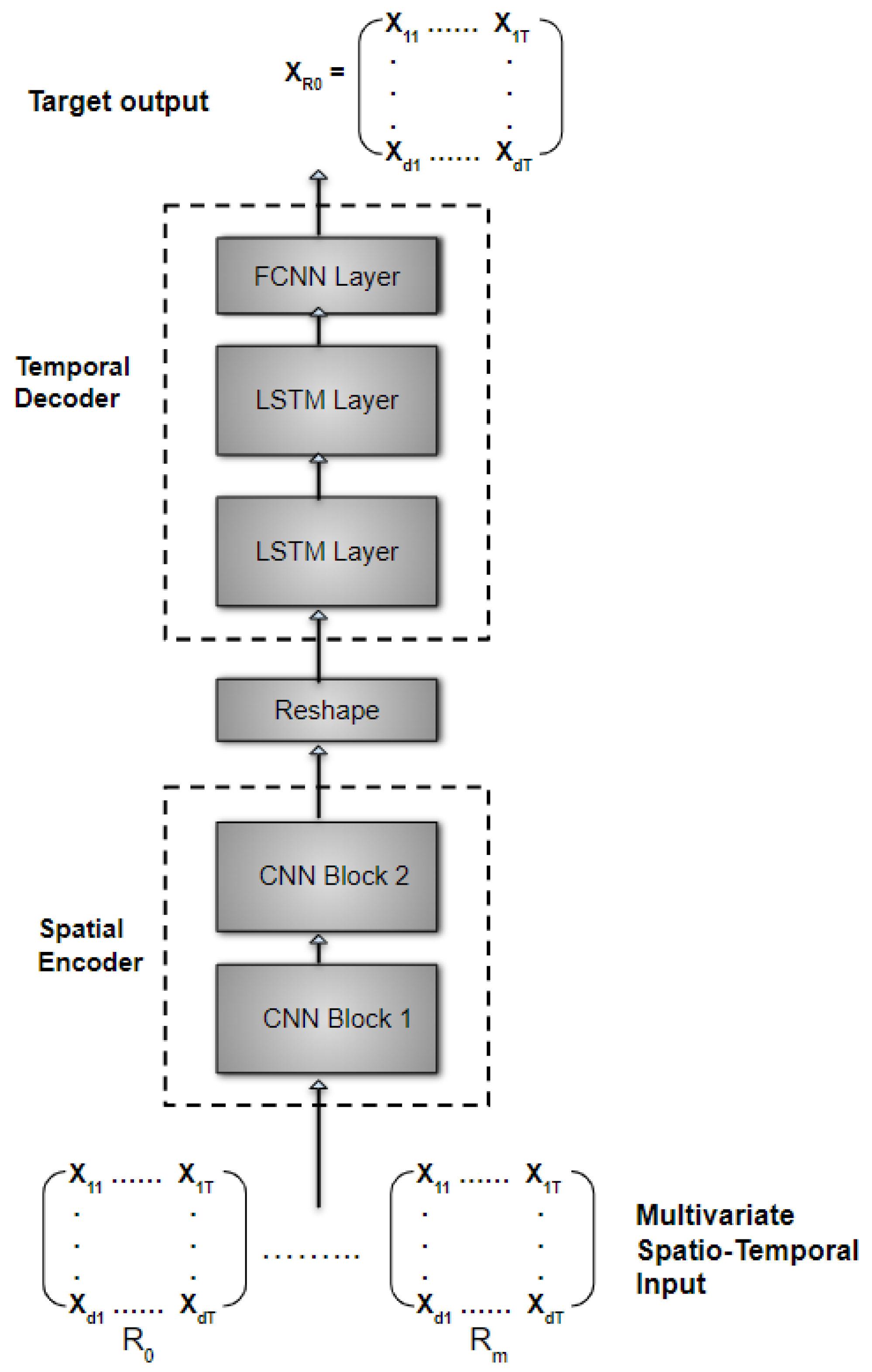
MC-CNN-Encoder component is composed of two convolutional blocks, and each block is made up of four cascading layers: 2D convolution kernel layer, followed by an activation layer, followed by 2D max-pooling layer and a channel-wise batch normalization layer. The first convolutional layer has 16   filters of size ( 2 × 2 ) with zero-padding and no striding (or with strides ( 1 × 1 ) ). The second convolution block has convolutional layer with 32   filters of size ( 3 × 3 ) without striding and with zero padding. The max pooling operation with pool size (2 × 2) and strides (2 × 2) is used to cut temporal dimensions by half at each max pooling layer.
The MC-CNN-Encoder takes three-dimensional multivariate spatio-temporal input data and generates a higher order representation of it. The dimension of the output of the MC-CNN-Encoder is ( t i m e s t a m p s × f e a t u r e s × f e a t u r e   m a p s ). Thus, we need to add a layer to reshape the output before passing to the LSTM layer. The output of the MC-CNN-Encoder is flattened over spatial dimensions into a feature vector and sent to the LSTM Decoder. As we go deeper in the network, the width and height dimensions (the temporal and feature dimensions representing multivariate time series) tend to shrink as a result of max pooling operation, while the number of feature maps (spatial dimension) for each Conv2D layer controlled by number of filters increases. This architecture helps to extract complex spatio-temporal dependencies for each data point in the dataset.

4.3.2. LSTM-Decoder

The spatial feature maps generated by the MC-CNN-Encoder are temporally dependent on previous time steps. An LSTM-Decoder is designed to represent those temporal dependencies. It decodes the MC-CNN-Encoder output and reconstructs the sequence data using hidden states (feature maps). It is composed of an LSTM block and a fully connected neural network (FCNN) layer. The LSTM block comprises of two LSTM layers followed by a dropout layer. The output of the LSTM block is fed to the FCNN layer, where the output is mapped into the feature set we want to reconstruct.
During the process of anomaly detection, the MC-CNN-Encoder learns a three-dimensional vector representation of the multivariate spatio-temporal input data. Then, the LSTM-Decoder uses the reshaped representation to extract temporal features and reconstruct the input data. The LSTM-block is trained to learn higher level temporal features of the input data, whereas the FCNN layer is trained to reconstruct the target univariate time series. In the LSTM block, two hidden layers are used with 64 and 16 hidden units each and followed by a dropout layer to prevent overfitting.
For the final dense (FCNN) layer, the number of units is set to d and it equals to the number of univariate time series (features) that we want to reconstruct. The number of hidden units in the dense layer can be adjusted according to the problem context at hand. For an anomaly detection problem, we are only interested with the reconstruction of a subset of original spatio-temporal multivariate dataset and not the fully reconstructed version of it. The overall framework is trained to produce the target multivariate time series X = { x 1 ,   ,   x T } of length T which is the size of the reconstruction window. The length of T can be equal to or smaller than the input window size T and should be tuned for each problem. Each sequence x i   d is an d -dimensional vector where d   d . The detailed architecture of the MC-CNN-Encoder and LSTM-Decoder are illustrated in Figure 4.

5. Experiments

To verify and evaluate the proposed hybrid deep learning framework for spatio-temporal anomaly detection, a set of experiments were conducted on buoy dataset. We used the year 2005 Gulf of Mexico (West) buoy dataset from National Buoy Data Center. A buoy is a floating object in water and used to mark the location and to record oceanographic data. Our main motivations in selecting this dataset and doing this case study can be given as:
  • Due to the difficulty of finding a labelled spatio-temporal multivariate real-world dataset for anomaly detection, we decided to use the buoy dataset full with well-known natural phenomena (anomalies) such as hurricanes.
  • Associating the spatio-temporal outliers detected between August 25th and August 30th with the path of Hurricane Katrina helps us to compare our approach with other algorithms.
  • To get a better understanding about the performance of algorithms, we used OAHII (Outliers Association with Hurricane Intensity Index) measures developed by Duggimpudi et al. [6] using the same buoy dataset. Using these measures, we were able to quantitatively compare the anomaly scores generated by algorithms.

5.1. Dataset Description

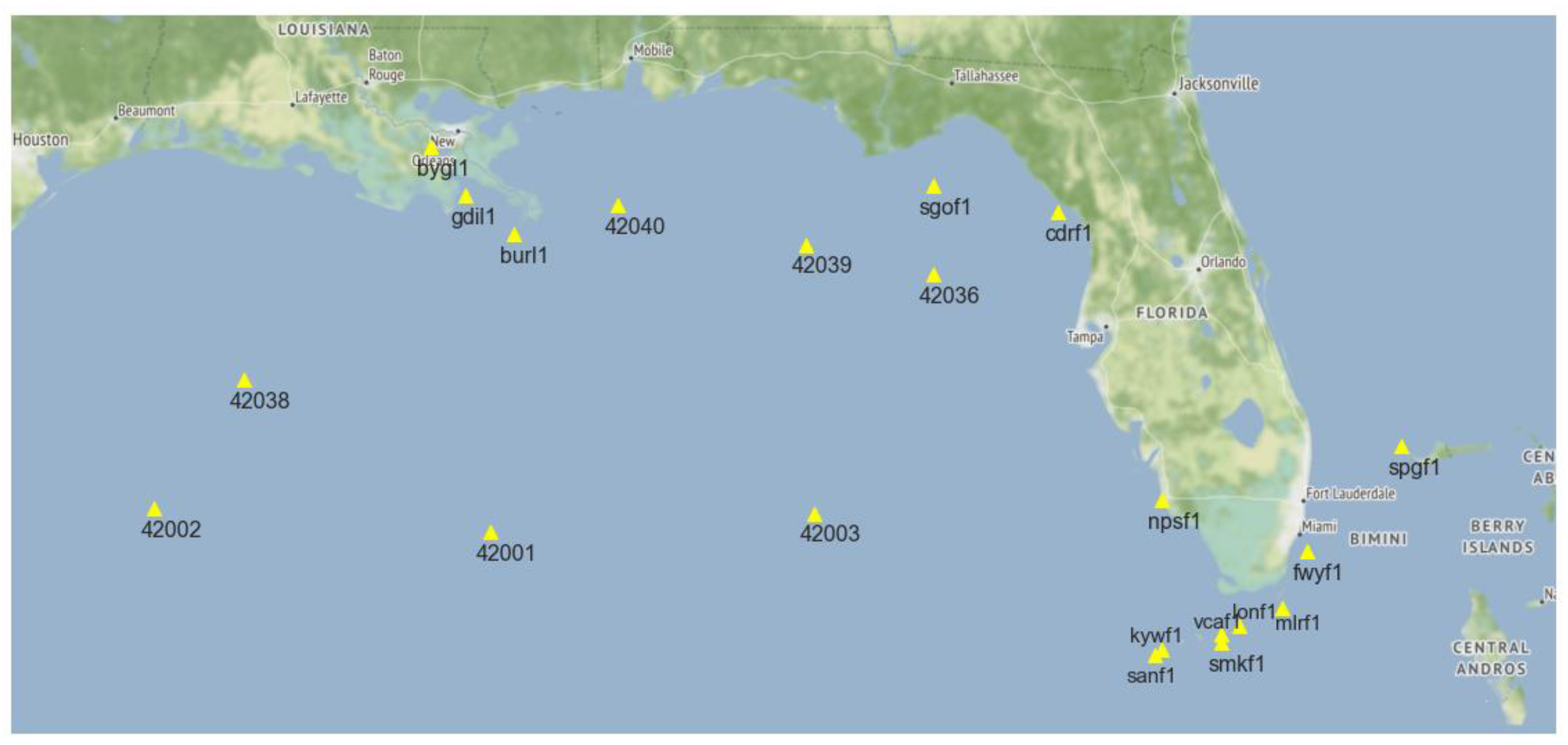
The buoy dataset has many meteorological measurements such as wind direction, wind speed, gust speed, wave height, air temperature, water temperature, tide, etc. However, buoy measurements from the year 2005 have many missing values or missing features. We have selected buoys which have sufficient historical data from the 2005 hurricane season for comparison purposes. For each buoy data reading, there are two contextual attributes: a time stamp (temporal context) attribute and latitude-longitude (spatial context) attribute which is static for each buoy. Beside these contextual attributes there are six behavioral attributes which are mostly available for each buoy used for this experiment: wind direction, wind speed, gust speed, barometric pressure, air temperature, and water temperature. After having eliminated buoys with many missing features and/or values and the ones that were damaged during the hurricane season we have selected 21 buoys and their data were included in our experiment. Those buoys are: 41001, 42001, 42003, 42036, 42038, 42039, 42040, FWYF1, BURL1, BYGL1, CDRF1, FWYF1, GDIL1, MLRF1, SANF1, SGOF1, SMKF1, SPGF1, VCAF1, KYWF1, NPSF1, and LONF1. Their locations are depicted in Figure 5. Python programming language and Geopandas (http://geopandas.org/), which is an open source project to work with geospatial data in Python, are used to depict buoy locations on map.

5.2. Data Preparation

Most buoys have hourly readings while some have readings in every 30 or 6 minutes. In such cases, we have down sampled data by selecting only hourly readings and discarding the rest to generate maximum 24 readings for each day. If a buoy has no reading corresponding to an hour, we fill the missing reading with a data point which was read less than 30 min ago.
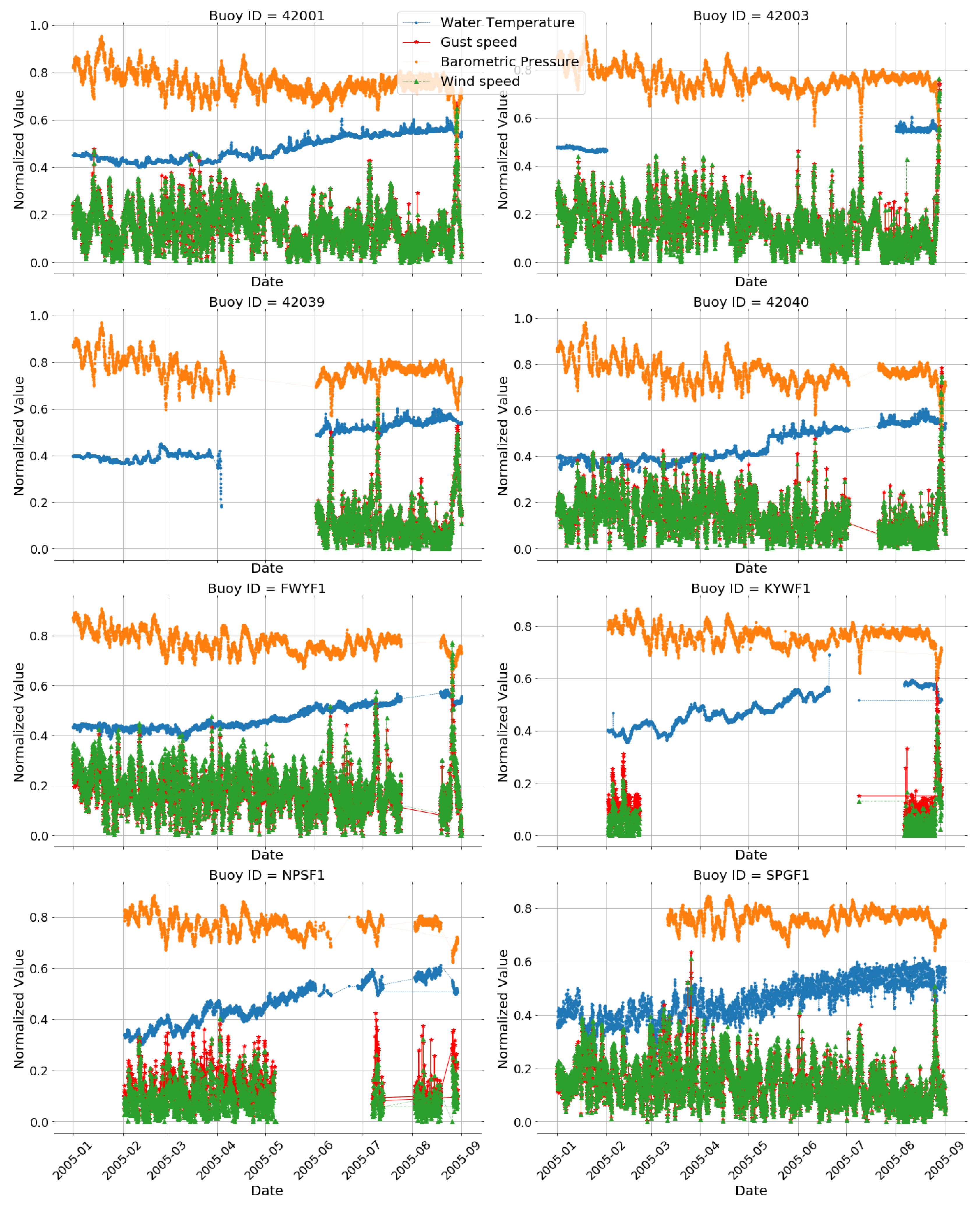
If there was a missing reading for any of the attributes in the historical data, it was imputed by National Data Buoy Center using any of the following values depending on the attribute: 99.00, 999.0, or 9999.0. We have imputed these missing observations by using piecewise linear interpolation technique by putting a limit of 24 (one day of data) on a maximum number of consecutive missing values that could be filled. Even after interpolation, there is still huge number of missing attributes for some of buoys as can be seen in Figure 6.
The wind direction attribute is defined as “the direction the wind is coming from in degrees clockwise from true N” by National Data Buoy Center and it takes values between 0° and 360°. In this study, we have divided the full 360° value into eight equally sized slices of 45° and label encoded each slice. Then, wind speed attribute of observations from buoys were one-hot encoded using these labels based on which slice direction its value falls in. Meanwhile, we have applied the min–max scaling technique on five attributes, which are water temperature (WTMP), air temperature (ATMP), wind speed (WSPD), gust speed (GST) and barometric pressure (BAR), to map all values to the range of [ 0 ,   1 ] .
We consider all data readings starting from January 1st, 2005 00:00 till August 31st, 2005 23:59; separating data from January till the end of June as training set, data from July as validation set and data from August as test set. We need all selected attribute values available for all data points to train models. We have discarded any observations with missing attributes, resulting a total of 93,982 readings from 21 different buoys. In the final dataset, the total number of data points is different for each buoy as the number of missing attributes differs significantly. In the final dataset, the number of data readings from each buoy is shown in Table 1, in column “# Observations”.
Training is executed using overlapping sequences obtained with a sliding window algorithm with a window size T and step size of s. The sliding window technique applied to the pre-processed buoy dataset to extract subsequences is given in Algorithm 1. The length of each subsequence is equal to the window size. Using sliding window technique, for a long sequence with length L, the number of extracted subsequences can be given as ⌈(L-T+1)/s⌉. This gives the maximum number of subsequences we can possibly extract. As shown in Figure 6, each buoy has a different number of missing data which results in data sequences with different length. Due to the high number of missing readings, we have tolerated missing data points on some time stamps by keeping the time difference limit between the end points of a subsequence at 2 × T. After having applied Algorithm 1 with window size set to 12 and step size to 1, we have generated training, validation and test sets which have different number of subsequences for each buoy as shown in Table 1.

5.3. Algorithms Used for Comparison

To validate the effectiveness of our approach, we have examined spatio-temporal outliers detected by our model and by the following state-of-the art anomaly detection techniques: ST-Outlier detection algorithm [5], ST-BDBCAN [6], LDBSCAN [8], LOF [9], and Isolation Forest [10]. We have implemented ST-Outlier detection and LDBSCAN algorithms in Python 3.6.8 programming language. For LOF (https://scikit-learn.org/stable/modules/generated/sklearn.neighbors.LocalOutlierFactor.html) and IsolationForest (https://scikit-learn.org/stable/modules/generated/sklearn.ensemble.IsolationForest.html) methods, we used implementations available in the scikit-learn (https://scikit-learn.org/stable/), which is a free machine learning library for Python programming language. We have used Euclidean distance for all proximity-based clustering algorithms since it has generated better results compared to other distance metrics. As ST-Outlier detection algorithm does not return a score, it is not included in the quantitative evaluation tests.
Model parameters were selected through randomized search over a predefined list for each parameter. For LDBSCAN algorithm, following values were assigned to the parameters since they gave the best result, as stated in [6]: LOFUB = 4, MinPtsLOF = 180, MinPtsLDBCAN = 225, and pct = 0.27. For the LOF algorithm, we used 50 for number of neighbors to use for k-nearest neighbor calculations, and 0.1 for contamination ratio. For the ST-Outlier detection algorithm, the following values were assigned to the parameters: Eps1 = 100 (distance parameter for spatial attribute), Eps2 = 0.2 (distance parameter for non-spatial attribute), MinPts = 5, which is the minimum number of points within Eps1 and Eps2 distance of a point. For IsolationForest, we have used 100 base estimators (number of trees), and contamination was set to 0.1.
Besides the above baseline methods, we also evaluate the depth of the components of the framework for the sample dataset: Number of layers in MC-CNN-Encoder component and number of layers in LSTM-decoder component. The quantitative evaluation of variants of the framework is given in the Section 5.5.3.
In order to compare our approach quantitatively to models which return an outlierness score, we have used three different OAHII (Outliers Association with Hurricane Intensity Index) measures developed by Duggimpudi et al. [6]. OAHII measures show how much the generated scores for each observation are correlated with the impact of the ground truth spatio-temporal anomaly which is the Hurricane Katrina for the test data. While OAHII1 measures the Pearson correlation between the outlierness score and actual impact of the hurricane on each data point and impact, OAHII2 measures the recall power of models using the impact vector as weight factor in weighted correlation, a derivative of Pearson correlation, and OAHII3 measures the precision power of models using the scores vector as weight vector in weighted correlation.

5.4. Framework Tuning

The proposed framework is implemented using the Keras (https://keras.io/) deep learning library using Python, running on top of the Tensorflow (https://www.tensorflow.org/) backend. All hidden layers are equipped with the Rectified Linear Unit (ReLU) non-linearity which allows the networks to converge faster [53]. For the final fully connected neural network layer, the sigmoid non-linear activation function is used. Optimization is performed by ADAM optimizer algorithm [54]. The Adam optimization algorithm is a powerful extension to stochastic gradient descent and has been successfully applied into deep learning applications in various domains such as computer vision and natural language processing. Layer weights are initialized with the Glorot uniform initializer. The framework is trained in mini-batches of size 32 for 20 epochs, with learning rate = 0.001, beta_1 = 0.9, beta_2 = 0.999, and epsilon = 1e-07. The final framework has 35,092 parameters to optimize. The optimum parameters for training epochs, batch size, learning rate and activation function are selected through grid search. Although window size is an important hyper parameter for time series analysis, our framework is not very sensitive to it, as it is explained in the next section. We have tested the performance of the proposed framework using window sizes 12, 6, and 3. The anomaly detection results given in Section 5.5.1 were generated by the framework with window size set to 12 (T = 12) and sliding step size set to 1.
Algorithm 1 Sliding window algorithm used in subsequence generation
#
p: current spatial context (e.g., sensor)
#
L: Full time series of current spatial context (multivariate)
#
T: window size
#
s: sliding step size
#
d: number of channels (depth of 3d spatio-temporal data matrix)
#
seqs: 3D tensor data for the current spatio-temporal data point
1:
function seqs = ExtractSubsequences(p, L, T, s, d)
2:
 start_indx = 0
3:
 end_indx = start_indx + T
4:
n = 0   # n is the number of subsequences
5:
 neighbour_list = getNearestNeighbours(p, d-1)
6:
 while (end_indx < length(L)):
7:
  # get timestamp of data at start_indx and end_indx
8:
  start_date_time = getTimestamp(L, start_indx)
9:
  end_date_time = getTimestamp(L, end_indx)
10:
  # check if there is a big time gap between start and end indexes
11.
  If  (end_date_time - start_date_time) < (2 × T):
12.
    # get the subsequence from the long time series data
13.
    seqs[n, 0] = L[start_indx..end_indx]
14.
    # get data from (d-1) nearest neighbours and attach to seqs
15.
    seqs[n, 1:d] = getDataFromNeighbours(T,
16.
                        start_date_time,
17.
                      end_date_time,
18.
                      neighbour_list)
19.
    start_indx = start_indx + s
20.
    end_indx = start_indx + T
21.
    n = n + 1
22.
 return seqs

5.5. Results

5.5.1. Anomaly Detection Results

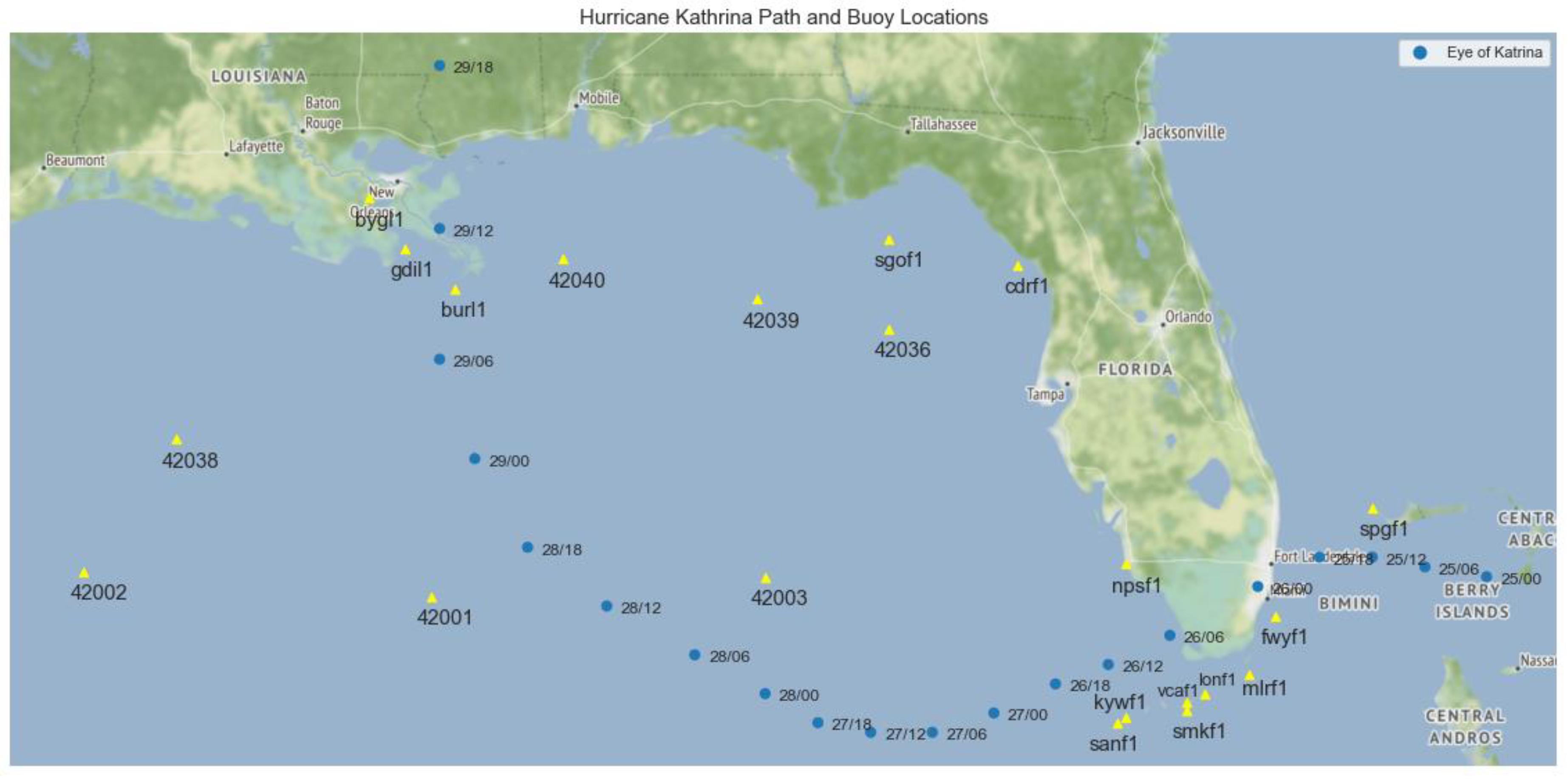
In Figure 7, the location of buoys and path of Hurricane Katrina along with the time stamps are shown. The track of Katrina is plotted according to “best track” positions and intensities measured in every six hours, which starts on 00:00 UTC 25 August and ends on 18:00 UTC 29 August [13]. The cyclone became Katrina, the 11th tropical storm of the 2005 Atlantic hurricane season, at 12:00 UTC 24 August when it was over the central Bahamas. Katrina has reached hurricane status near 21:00 UTC 25 August, less than two hours before its center made landfall on the southeastern coast of Florida. As it entered the Gulf of Mexico on 26 August, Katrina entered two rapid intensification periods between 26 and 28 August. Katrina strengthened from a low-end Category 3 hurricane to a Category 5 in less than 12 hours reaching the peak by 12:00 UTC 28 August. The large wind field on 28 August, with hurricane-force winds extended out to about 90 nautical miles from the center, made Katrina extremely intense and exceptionally large [13].
The center of Katrina passed by the buoy 43003 on 06:00 UTC 28 August, the buoy 42001 on 18:00 UTC 28 August, and the buoy 42040 on 09:00 UTC 29 August. The timestamps of top five scoring spatio-temporal anomalous data points detected by algorithms for buoys 42001, 42003, and 42040 are given in Table 2. The anomalies which are in space-time vicinity of the Hurricane Katrina are given in blue for performance comparison. The proposed framework (MC-CNN-LSTM) with window size 12 detected all spatio-temporal anomalies caused by Hurricane Katrina as it passed by buoys. When we examine the results, LDBSCAN seems to give the highest score to data points which are the most related with Hurricane Katrina path after our model, followed by the ST-Outlier detection algorithm, LOF and IsolationForest.
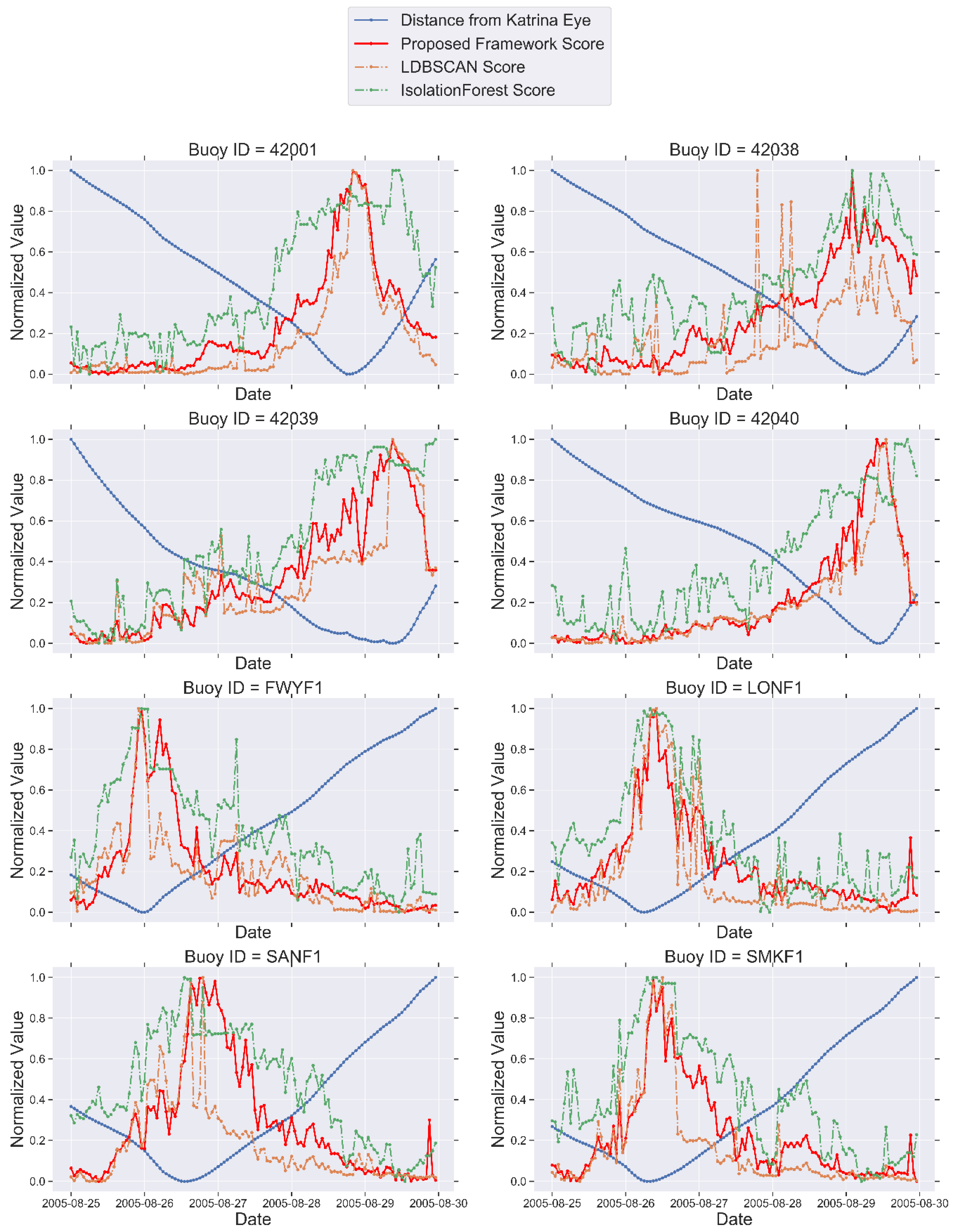
Although this heuristic analysis gives a high-level understanding about performance of algorithms, it is better to take all data points and their scores into account for the duration of Hurricane Katrina. The actual Katrina path reported by Knabb et al. [13] gives latitude and longitude information of the center reported for every six hours. We have applied linear interpolation to transform it to an hourly basis data to match the buoys’ hourly readings data. For each buoy whose location is highly relevant to Katrina’s path, we have plotted the anomaly score of each data point against the distance to the center of the Katrina for the time frame starting on 00:00 UTC 25 August and ending on 23:59 UTC 29 August. In order to show comparison in detail, anomaly scores of the proposed framework (MC-CNN-LSTM), LDBSCAN and IsolationForest algorithms are plotted against the distance between buoys and the center of the Katrina in Figure 8. Anomaly score values and distances are min-max normalized in the range of [0, 1] before plotting.
In Figure 8, we can observe that the anomaly scores of LDBSCAN and IsolationForest are not stable and results contain many false positives and false negatives. For the LDBSCAN algorithm, false alarms based on generated anomaly scores are quite visible for buoys 42038, LONF1, and SANF1. For buoy 42038, LDBSCAN generates three highest scores for data points when Katrina center is not the closest. For buoys LONF1 and SANF1, LDBSCAN exhibits high anomaly score values followed by sharp drops which followed by high score values again for data points when Katrina center is very close. On the other hand, IsolationForest, which is the next best performing algorithm according to the results of quantitative evaluation given in Section 5.5.2, shows weaker performance than the proposed framework in capturing the anomalous trend in the test data. Its performance degrades significantly for buoys FWYF1, SANF1, and SMKF1. Although these buoys are on the direct path of the Katrina, anomaly scores generated by IsolationForest are not stable and exhibit high values for data points when Katrina center is not very close. Meanwhile, the anomaly scores generated by MC-CNN-LSTM is smoother than LDBSCAN and IsolationForest. In other words, the anomaly scores generated by MC-CNN-LSTM do not exhibit sharp drops and high peaks in consecutive data points. The proposed framework outperforms LDBSCAN and IsolationForest in capturing the overall anomalous trend in the test data. In summary, MC-CNN-LSTM generates fewer false alarms and does not miss real alarms, as generated anomaly score values show higher correlation with the distance between buoys and the center of the Katrina.

5.5.2. Quantitative Evaluation of Models

To provide a further quantitative evaluation, we have used the measure OAHII (Outliers Association with Hurricane Intensity Index) developed by Duggimpudi et al. [6]. OAHII shows how much correlation exists between the outlierness scores generated by an algorithm and the actual impact of the hurricane (which is the ground truth for the given dataset). The ground truth is represented by the actual Katrina path reported in Knabb et al. [13], which contains the best track positions and intensities reported once every 6 h. It contains the latitude, longitude, time, wind speed and pressure information around a set of hurricane eye locations during the period from August 23rd to August 31st. We have applied linear interpolation to the ground truth data to fill missing hurricane readings and to transform it to an hourly basis like the buoy dataset.
The anomaly scores of the proposed hybrid deep learning framework (HDLF) and IsolationForest (IF), LDBSCAN, LOF, and ST-BDBCAN algorithms are compared, excluding ST-Outlier detection algorithm as it does not generate a score. The proposed framework is tested against the data prepared with different window sizes to demonstrate that it is the highest performing model at each configuration. We used Euclidean distance for LOF and LDBSCAN algorithms as it gives better results. However, we gave the result for ST-BDBCAN generated by using Mahalanobis distance since it yielded in better results as indicated by Duggimpudi et al. [6]. Results of the three OAHII measures, OAHII1, OAHII2, and OAHII3 are shown in Table 3.
OAHII measures show the effectiveness of our model over the state-of-the art spatio-temporal anomaly detection algorithms. It is superior to other approaches in terms of both anomaly detection accuracy, which is given in Table 2, and correlation of scores to the ground truth, which is given in Table 3. According to the results given in Table 3, our model performed better than the next best performing algorithm in detecting anomalies scoring more than 10% in all OAHII measures.

5.5.3. Quantitative Evaluation of Framework Variants

To further investigate the effects of hyper parameters, we have tested the framework under different configurations by changing the number of CNN and LSTM layers. The following variants of the proposed framework were tested: CNN(1)-LSTM(1), CNN(1)-LSTM(2), CNN(1)-LSTM(3), CNN(2)-LSTM(1), CNN(2)-LSTM(2), CNN(2)-LSTM(3), CNN(3)-LSTM(1), CNN(3)-LSTM(2), CNN(3)-LSTM(3), numbers in parenthesis representing the number of layers. Only OAHII1 measure is considered for this experiment. Data are preprocessed using the window size T = 12 and with different sliding step sizes s = 1, 2, 3, 4, 6, 12. The quantitative evaluation results of framework variants are given in Table 4.
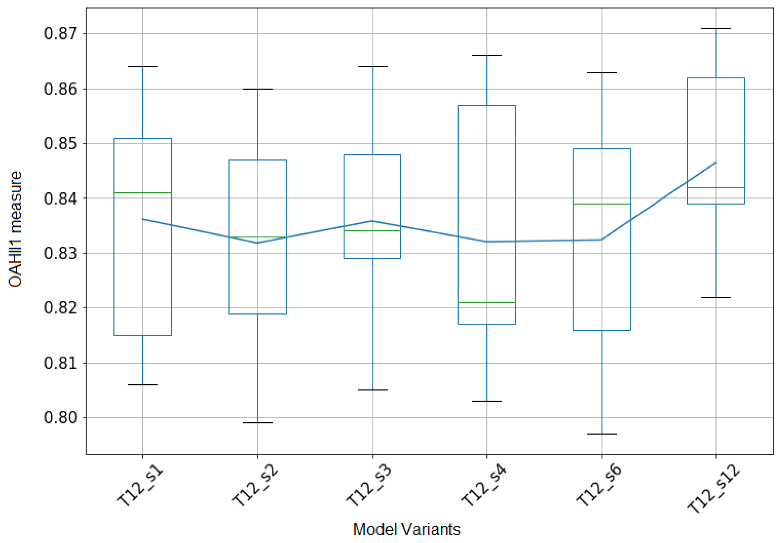
The best OAHII1 measure for each framework variant is given in blue. The overall results show that for the given problem domain the network is not very sensitive to the number of layers and increasing the number of layers does not improve the performance significantly. The boxplot of each framework variant is given in Figure 9. According to the mean score of each model variant represented by the blue line in the box plot, the accuracy (OAHII1 measure) does not deviate much between different models with different network parameters. The average accuracy calculated over all framework variants with different step sizes is 0.836 and more than 10% better than the next best scoring algorithm, which is IsolationForest according to the quantitative evaluation results given in Table 3. The core architecture of the network and the way we use the spatial and temporal context prove to be a powerful approach in spatio-temporal anomaly detection problem.

6. Discussions

In this study, a new hybrid approach is proposed to the problem of unsupervised anomaly detection in multivariate spatio-temporal data. In unsupervised scenarios, the type of anomalies and the ratio of anomalous events within the given dataset are generally not known. Training data might be contaminated by anomalous data which is the case in most of the real word scenarios. For the proposed unsupervised setting, no labeled dataset is required to train the framework for the anomaly detection problem. The proposed hybrid deep learning framework is designed to be trained in a truly unsupervised fashion with the full absence of labels, for either normal or abnormal data. It is composed of a multi-channel convolutional neural network (CNN) and Long Short-Term Memory (LSTM) network. The architecture of the framework is based on an autoencoder scheme: the multi-channel CNN network is deployed on the encoder side for learning spatial structures of each spatio-temporal multivariate data frame, and LSTM network is deployed on the decoder side for learning temporal patterns from the encoded spatial structures. The architecture is robust enough to learn the important structure of the data even if the training dataset contains noise and anomalous data points. To the best of our knowledge, this is the first deep learning-based approach for unsupervised anomaly detection problem in non-image multivariate spatio-temporal dataset.
A set of experiments was carried out using the buoy dataset from National Data Buoy Center which is contaminated with noise and anomalies such as tropical storms and hurricanes. We demonstrated that the proposed encoder–decoder-based architecture achieves better results against state-of-the-art spatio-temporal anomaly detection methods providing at least 10% improvement in quantitative scores. The proposed hybrid model stands out from other traditional and deep learning-based models as it is capable of handling noise and missing values better. Quantitative evaluation tests of framework variants show that the core architecture of the network and the way we use the spatial and temporal context prove to be a powerful and robust approach in the spatio-temporal anomaly detection problem.
The major contributions of this study can be summarized as follows:
  • In the proposed hybrid model, we handle spatial and temporal contexts by different deep learning components as these contextual variables refer to different types of dependencies.
  • Unlike proximity-based methods, the proposed model can be easily implemented on datasets with mixed-type behavioral attributes and it scales well to multivariate datasets with high number of features.
  • The crafting of multivariate spatio-temporal dataset for unsupervised anomaly detection is also novel. The multi-channel CNN encoder network provides better representative spatial features for the anomaly detection process by using spatial neighborhood data.
We believe that this approach is an important improvement towards applying deep learning in unsupervised learning problems. In the future, we plan to broaden this study in several directions. First, we plan to enhance the framework by adding the attention mechanism to tackle the weaknesses in analyzing long sequences. By letting the decoder component to have an attention mechanism, we believe that the framework can better detect collective anomalies in long ranging multivariate spatio-temporal data. Second, we also plan to explore optimization-based techniques to select framework’s hyper-parameters to further enhance the performance. Finally, we would like to conduct research on more efficient data imputation techniques to improve the anomaly detection process for real life datasets.

Author Contributions

Conceptualization, Y.K.; methodology, Y.K.; software, Y.K.; validation, Y.K.; formal analysis, Y.K.; investigation, Y.K.; resources, Y.K.; data curation, Y.K.; writing—original draft preparation, Y.K.; writing—review and editing, Y.K., M.N.A. and A.S.Ö.; visualization, Y.K.; supervision, M.N.A. and A.S.Ö.; project administration, Y.K., M.N.A. and A.S.Ö. All authors have read and agreed to the published version of the manuscript.

Funding

This research received no external funding.

Conflicts of Interest

The authors declare no conflict of interest.

References

  1. Gupta, M.; Gao, J.; Aggarwal, C.C.; Han, J. Outlier Detection for Temporal Data: A Survey. IEEE Trans. Knowl. Data Eng. 2014, 26, 2250–2267. [Google Scholar] [CrossRef]
  2. Cheng, T.; Li, Z. A Multiscale Approach for Spatio-temporal Outlier Detection. Trans. GIS. 2006, 10, 253–263. [Google Scholar] [CrossRef]
  3. Aggarwal, C.C. Spatial Outlier Detection. In Outlier Analysis, 2nd ed.; Springer Nature: New York, NY, USA, 2017; pp. 345–367. [Google Scholar]
  4. Hodge, V.J.; Austin, J. A Survey of Outlier Detection Methodologies. Artif. Intell. Rev. 2004, 22, 85–126. [Google Scholar]
  5. Birant, D.; Kut, A. Spatio-temporal outlier detection in large databases. J. Comput. Inform. Technol. 2006, 14, 291–297. [Google Scholar] [CrossRef] [Green Version]
  6. Duggimpudi, M.B.; Abbady, S.; Chen, J.; Raghavan, V.V. Spatio-temporal outlier detection algorithms based on computing behavioral outlierness factor. Data Knowl. Eng. 2019, 122, 1–24. [Google Scholar] [CrossRef]
  7. Ester, M.; Kriegel, H.P.; Sander, J.; Xu, X. A density-based algorithm for discovering clusters in large spatial databases with noise. In Proceedings of the Second International Conference on Knowledge Discovery and Data Mining, Portland, OR, USA, 2–4 August 1996; pp. 226–231. [Google Scholar]
  8. Duan, L.; Xu, L.; Guo, F.; Lee, J.; Yan, B. A local-density based spatial clustering algorithm with noise. Inform. Syst. 2007, 32, 978–986. [Google Scholar] [CrossRef]
  9. Breunig, M.M.; Kriegel, H.P.; Ng, R.T.; Sander, J. LOF: Identifying Density-Based Local Outliers. In Proceedings of the ACM SIGMOD 2000 International Conference on Management of Data, Dallas, TX, USA, 16–18 May 2000; pp. 93–104. [Google Scholar]
  10. Liu, F.T.; Ting, K.M.; Zhou, Z.H. Isolation Forest. In Proceedings of the Eighth IEEE International Conference on Data Mining, Pisa, Italy, 15–19 December 2008; pp. 413–422. [Google Scholar]
  11. Liu, F.T.; Ting, K.M.; Zhou, Z.H. Isolation-based anomaly detection. ACM Trans. Knowl. Discov. 2012, 6, 31–39. [Google Scholar] [CrossRef]
  12. Aggarwal, C.C. Linear Models for Outlier Detection. In Outlier Analysis, 2nd ed.; Springer Nature: New York, NY, USA, 2017; pp. 65–110. [Google Scholar]
  13. Knabb, R.D.; Rhome, J.R.; Brown, D.P. Tropical Cyclone Report: Hurricane Katrina, 23–30 August 2005. National Hurricane Center. Available online: https://www.nhc.noaa.gov/data/tcr/AL122005_Katrina.pdf (accessed on 16 October 2019).
  14. Yaminshi, K.; Takeuchi, J. A unifying framework for detecting outliers and change points from non-stationary time series data. In Proceedings of the Eighth ACM SIGKDD International Conference on Knowledge Discovery and Data Mining, Edmonton, AB, Canada, 23–26 July 2002; pp. 676–681. [Google Scholar]
  15. Cheng, H.; Tan, P.N.; Potter, C.; Klooster, S. Detection and Characterization of Anomalies in Multivariate Time Series. In Proceedings of the 2009 SIAM International Conference on Data Mining, Sparks, NV, USA, 30 April–2 May 2009. [Google Scholar]
  16. Shekhar, S.; Lu, C.-T.; Zhang, P. A Unified Approach to Detecting Spatial Outliers. GeoInformatica 2003, 7, 139–166. [Google Scholar] [CrossRef]
  17. Lu, C.-T.; Chen, D.; Kou, Y. Algorithms for spatial outlier detection. In Proceedings of the Third IEEE International Conference on Data Mining, Melbourne, FL, USA, 19–22 November 2003; pp. 597–600. [Google Scholar]
  18. Shekhar, S.; Lu, C.-T.; Zhang, P. Detecting Graph-based Spatial Outliers: Algorithms and Applications. In Proceedings of the 7th ACM SIGKDD International Conference on Knowledge Discovery and Data Mining, San Francisco, CA, USA, 26–19 August 2001; pp. 371–376. [Google Scholar]
  19. Sun, P.; Chawla, S. On local spatial outliers. In Proceedings of the Fourth IEEE International Conference on Data Mining, Brighton, UK, 1–4 November 2004; pp. 209–216. [Google Scholar]
  20. Gupta, M.; Sharma, A.B.; Chen, H.; Jiang, G. Context-Aware Time Series Anomaly Detection for Complex Systems. In Proceedings of the SDM Workshop of SIAM International Conference on Data Mining, Austin, TX, USA, 2–4 May 2013. [Google Scholar]
  21. Jolliffe, I.T. Principal Component Analysis, 2nd ed.; Springer: New York, NY, USA, 2002; pp. 1–76. [Google Scholar]
  22. Aggarwal, C.C.; Reddy, C.K. Data Clustering: Algorithms and Applications, 1st ed.; CRC Press: Boca Raton, FL, USA, 2013; pp. 88–106. [Google Scholar]
  23. Alonso, F.; Ros, M.C.V.; Castillo, F.G. Isolation Forests to Evaluate Class Separability and the Representativeness of Training and Validation Areas in Land Cover Classification. Remote Sens. 2019, 11, 3000. [Google Scholar] [CrossRef] [Green Version]
  24. Chen, C.; Zhang, D.; Castro, P.S.; Li, N.; Sun, L.; Li, S.; Wang, Z. iBOAT: Isolation-Based Online Anomalous Trajectory Detection. IEEE Trans. Intell. Transp. Syst. 2013, 14, 806–818. [Google Scholar] [CrossRef]
  25. Stripling, E.; Baesens, B.; Chizi, B.; Broucke, S. Isolation-based conditional anomaly detection on mixed-attribute data to uncover workers’ compensation fraud. Decis. Support. Syst. 2018, 111, 13–26. [Google Scholar] [CrossRef]
  26. Malhotra, P.; Ramakrishnan, A.; Anand, G.; Vig, L.; Agarwal, P.; Shroff, G. LSTM-based Encoder-Decoder for Multi-sensor Anomaly Detection. ICML 2016, Anomaly Detection Workshop. arXiv 2016, arXiv:1607.00148v2. [Google Scholar]
  27. Kim, T.-Y.; Cho, S.-B. Web traffic anomaly detection using C-LSTM neural networks. Expert Syst. Appl. 2018, 106, 66–76. [Google Scholar] [CrossRef]
  28. Zhang, C.; Song, D.; Chen, Y.; Feng, X.; Lumezanu, C.; Cheng, W.; Ni, J.; Zong, B.; Chen, H.; Chawla, N.V. A Deep Neural Network for Unsupervised Anomaly Detection and Diagnosis in Multivariate Time Series Data. arXiv 2018, arXiv:1811.08055. [Google Scholar] [CrossRef] [Green Version]
  29. Christiansen, P.; Nielsen, L.N.; Steen, K.A.; Jørgensen, R.N.; Karstoft, H. DeepAnomaly: Combining Background Subtraction and Deep Learning for Detecting Obstacles and Anomalies in an Agricultural Field. Sensors 2016, 16, 1904. [Google Scholar] [CrossRef] [Green Version]
  30. Oh, D.Y.; Yun, I.D. Residual Error Based Anomaly Detection Using Auto-Encoder in SMD Machine Sound. Sensors 2018, 18, 1308. [Google Scholar] [CrossRef] [Green Version]
  31. Munir, M.; Siddiqui, S.A.; Chattha, M.A.; Dengel, A.; Ahmed, S. FuseAD: Unsupervised Anomaly Detection in Streaming Sensors Data by Fusing Statistical and Deep Learning Models. Sensors 2019, 19, 2451. [Google Scholar] [CrossRef] [Green Version]
  32. Hinton, G.E.; Salakhutdinov, R.R. Reducing the Dimensionality of Data with Neural Networks. Science 2006, 313, 504–507. [Google Scholar] [CrossRef] [Green Version]
  33. Bengio, Y. Learning Deep Architectures for AI. Found. Trends Mach. Learn. 2009, 2, 1–127. [Google Scholar] [CrossRef]
  34. Hecht-Nielsen, R. Replicator Neural Networks for Universal Optimal Source Coding. Science 1995, 269, 1860–1863. [Google Scholar] [CrossRef]
  35. Japkowicz, N.; Hanson, S.; Gluck, M. Nonlinear autoassociation is not equivalent to PCA. Neural Comput. 2000, 12, 531–545. [Google Scholar] [CrossRef] [PubMed]
  36. Vincent, P.; Larochelle, H.; Lajoie, I.; Bengio, Y.; Manzagol, P.A. Stacked denoising autoencoders: Learning useful representations in a deep network with a local denoising criterion. J. Mach. Learn. Res. 2010, 11, 3371–3408. [Google Scholar]
  37. Rifai, S.; Vincent, P.; Muller, X.; Glorot, X.; Bengio, Y. Contractive auto-encoders: Explicit invariance during feature extraction. In Proceedings of the 28th International Conference on Machine Learning (ICML-11), Bellevue, WA, USA, 28 June–2 July 2011; pp. 833–840. [Google Scholar]
  38. Sakurada, M.; Yairi, T. Anomaly detection using autoencoders with nonlinear dimensionality reduction. In Proceedings of the MLSDA 2014 2nd Workshop on Machine Learning for Sensory Data Analysis, Gold Coast, Australia, 2 December 2014. [Google Scholar] [CrossRef]
  39. Goodfellow, I.; Bengio, Y.; Courville, A. Deep Learning, 1st ed.; MIT Press: Cambridge, MA, USA, 2016; pp. 493–549. [Google Scholar]
  40. LeCun, Y.; Bengio, Y. Convolutional networks for images, speech, and time series. In The Handbook of Brain Theory and Neural Networks; MIT Press: Cumberland, RI, USA, 1995; Volume 3361. [Google Scholar]
  41. Krizhevsky, A.; Sutskever, I.; Hinton, G.E. Imagenet classification with deep convolutional neural networks. In Proceedings of the Neural Information Processing Systems Conference, Lake Tahoe, NV, USA, 3–6 December 2012; pp. 1097–1105. [Google Scholar]
  42. Aggarwal, C.C. Convolutional Neural Networks. In Neural Networks and Deep Learning, 1st ed.; Springer International Publishing: Cham, Switzerland, 2018; pp. 315–373. [Google Scholar]
  43. Scherer, D.; Müller, A.; Behnke, S. Evaluation of Pooling Operations in Convolutional Architectures for Object Recognition. In Proceedings of the 20th International Conference on Artificial Neural Networks, Part III, Thessaloniki, Greece, 15–18 September 2010; Springer: Berlin/Heidelberg, Germany; pp. 92–101. [Google Scholar]
  44. Hochreiter, S.; Schmidhuber, J. Long short-term memory. Neural Comput. 1997, 9, 1735–1780. [Google Scholar] [CrossRef] [PubMed]
  45. Sutskever, I.; Vinyals, O.; Le, Q.V. Sequence to Sequence Learning with Neural Networks. Adv. Neural Inform. Proc. Syst. 2014, 27, 3104–3112. [Google Scholar]
  46. Graves, A.; Jaitly, N. Towards end-to-end speech recognition with recurrent neural networks. In Proceedings of the International Conference on Machine Learning, Beijing, China, 21–26 June 2014; pp. 1764–1772. [Google Scholar]
  47. Srivastava, N.; Mansimov, E.; Salakhutdinov, R. Unsupervised Learning of Video Representations using LSTMs 2015. arXiv 2015, arXiv:1502.04681v3. [Google Scholar]
  48. Wu, Z.; Wang, X.; Jiang, Y.G.; Ye, H.; Xue, X. Modeling Spatial-Temporal Clues in a Hybrid Deep Learning Framework for Video Classification. In Proceedings of the 23rd ACM International Conference, Seattle, WA, USA, 3–6 November 2015. [Google Scholar]
  49. Sainath, T.N.; Vinyals, O.; Senior, A.; Sak, H. Convolutional, Long Short-Term Memory, fully connected Deep Neural Networks. In Proceedings of the IEEE International Conference on Acoustics, Speech and Signal Processing, Brisbane, Australia, 19–24 April 2015; pp. 4580–4584. [Google Scholar]
  50. Zheng, Y.; Liu, Q.; Chen, E.; Ge, Y.; Zhao, J.L. Time Series Classification Using Multi-Channels Deep Convolutional Neural Networks. In Proceedings of the International Conference on Web-Age Information Management, Macau, China, 16–18 June 2014; pp. 298–310. [Google Scholar]
  51. Zheng, Y.; Liu, Q.; Chen, E.; Ge, Y.; Zhao, J.L. Exploiting multi-channels deep convolutional neural networks for multivariate time series classification. Front. Comput. Sci. 2016, 10, 96–112. [Google Scholar] [CrossRef]
  52. Wang, Z.; Yan, W.; Oates, T. Time series classification from scratch with deep neural networks: A strong baseline. In Proceedings of the International Joint Conference on Neural Networks, Anchorage, AK, USA, 14–19 May 2017; pp. 1578–1585. [Google Scholar]
  53. Simonyan, K.; Zisserman, A. Very deep convolutional networks for large-scale image recognition. arXiv 2014, arXiv:1409.1556v6. [Google Scholar]
  54. Kingma, D.P.; Ba, J. Adam: A Method for Stochastic Optimization. In Proceedings of the 3rd International Conference for Learning Representations, San Diego, CA, USA, 7–9 May 2015. [Google Scholar]
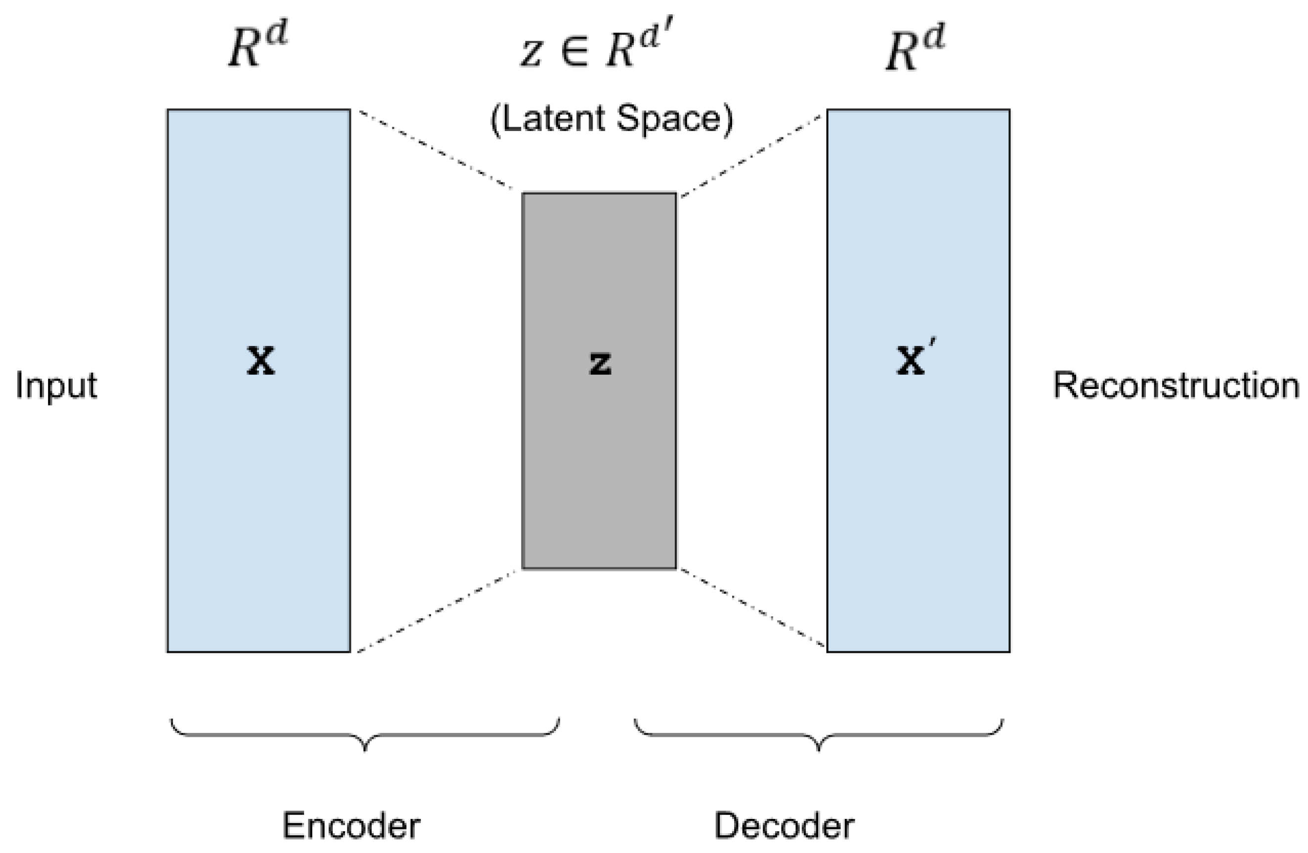
Figure 1. Illustration of an autoencoder.
Applsci 10 05191 g001
Figure 2. Illustration of the three-dimensional multivariate spatio-temporal data matrix structure.
Applsci 10 05191 g002
Figure 3. Overall architecture of the proposed hybrid deep learning framework. It has two main components: A multi-channel convolutional encoder (MC-CNN-Encoder) for spatial encoding and an LSTM-based decoder for temporal decoding.
Applsci 10 05191 g003
Figure 4. The detailed architecture of the hybrid autoencoder framework: It has a Convolutional Neural Network (CNN)-based spatial encoder and a Long Short-Term Memory (LSTM)-Fully Connected Neural Network (FCNN)-based temporal decoder.
Applsci 10 05191 g004
Figure 5. The location of buoys used in the experiment.
Applsci 10 05191 g005
Figure 6. Sample data from buoys 42001, 42003, 42039, 42040, FWYF1, KYWF1, NPSF1, and SPGF1 after interpolation. Attributes shown: Water temperature (WTMP), Gust speed (GST), Barometric Pressure (BAR), and Wind speed (WSPD).
Applsci 10 05191 g006
Figure 7. Buoy locations and path of Hurricane Katrina.
Applsci 10 05191 g007
Figure 8. Anomaly score comparison of the proposed framework, IsolationForest and the LDBSCAN algorithm. Normalized anomaly scores are plotted against the normalized distance between buoys and the center of the Katrina.
Applsci 10 05191 g008
Figure 9. Boxplot of OAHII1 measures of framework variants. Blue line represents mean scores.
Applsci 10 05191 g009
Table 1. Total number of observations belonging to each buoy and number of subsequences created for training, test, and validation sets.
Buoy ID# Observations# Training
Subsequences
# Validation
Subsequences
# Testing
Subsequences
42,00158224325731730
42,00258074295732725
42,00314217550642
42,03654524304372729
42,03858114316732715
42,0392178682730723
42,04053484297274723
BURL157604327732665
BYGL139532195697574
CDRF156254105732730
FWYF152314325565305
GDIL157824321732693
KYWF18803990444
LONF158254326732731
MLRF158274328732731
NPSF126382044100397
SANF158184323731728
SGOF155734268539730
SMKF136222124732730
SPGF141722674732730
VCAF11437108706573
Table 2. Timestamps of detected anomalies. Anomalous data points which are in the spatio-temporal neighborhood of the Hurricane Katrina are given in blue.
Buoy IDIsolationForestLOFLDBSCANST-Outlier
Detection
MC-CNN-LSTM (T = 12)
42,0012005-08-29 09:002005-08-28 20:002005-08-28 20:002005-08-27 08:002005-08-28 20:00
2005-08-29 10:002005-08-28 21:002005-08-28 21:002005-08-28 19:002005-08-28 21:00
2005-08-29 11:002005-08-28 19:002005-08-28 22:002005-08-28 20:002005-08-29 00:00
2005-08-29 12:002005-08-29 09:002005-08-29 00:002005-08-28 21:002005-08-28 22:00
2005-08-29 19:002005-08-29 11:002005-08-28 23:002005-08-31 23:002005-08-28 19:00
42,0032005-08-27 05:002005-08-07 20:002005-08-27 17:002005-08-24 20:002005-08-28 01:00
2005-08-27 03:002005-08-27 00:002005-08-28 01:002005-08-24 21:002005-08-28 04:00
2005-08-27 04:002005-08-27 06:002005-08-27 18:002005-08-24 22:002005-08-28 02:00
2005-08-28 05:002005-08-27 08:002005-08-27 16:002005-08-28 04:002005-08-28 03:00
2005-08-28 04:002005-08-27 09:002005-08-27 20:002005-08-28 05:002005-08-28 00:00
42,0402005-08-29 20:002005-08-29 16:002005-08-29 13:002005-08-29 12:002005-08-29 13:00
2005-08-29 16:002005-08-29 10:002005-08-29 12:002005-08-29 13:002005-08-29 12:00
2005-08-29 17:002005-08-29 09:002005-08-29 11:002005-08-29 14:002005-08-29 10:00
2005-08-29 18:002005-08-29 08:002005-08-29 14:002005-08-29 15:002005-08-29 11:00
2005-08-29 19:002005-08-29 23:002005-08-29 10:002005-08-31 19:002005-08-29 09:00
Table 3. Quantitative evaluation of algorithms.
ModelsIFLOFLDBSCANST-BDBCANHDLF
(T = 3)
HDLF
(T = 6)
HDLF
(T = 12)
Measures
OAHII10.7220.3860.6810.5950.8100.8230.866
OAHII20.7410.3270.6620.6640.7910.8220.856
OAHII30.6600.2100.4840.6320.7410.7700.843
Table 4. OAHII1 measures of the framework variants with window size T = 12 and different sliding step sizes s = 1, 2, 3, 4, 6, 12.
Model VariantsT = 12, s = 1T = 12, s = 2T = 12, s = 3T = 12, s = 4T = 12, s = 6T = 12, s = 12
CNN(1)-LSTM(1)0.8150.8330.8640.8570.8630.862
CNN(1)-LSTM(2)0.8640.8410.8340.8660.8530.841
CNN(1)-LSTM(3)0.8410.8470.8510.8570.7970.826
CNN(2)-LSTM(1)0.8150.8280.8180.8170.8490.871
CNN(2)-LSTM(2)0.8620.8110.8290.8420.8170.842
CNN(2)-LSTM(3)0.8510.8600.8320.8030.8410.839
CNN(3)-LSTM(1)0.8060.7990.8050.8070.8160.869
CNN(3)-LSTM(2)0.8300.8190.8410.8210.8390.846
CNN(3)-LSTM(3)0.8410.8480.8480.8180.8160.822