Energy-Based Prediction of the Displacement of DCFP Bearings

Abstract

Isolation systems are currently being widely applied for earthquake resistance. During the design stage for such systems, the displacement response and input energy of the isolation layer are two of the main concerns. The prediction of these values is also of vital importance during the early stages of the structural design. In this study, the simple prediction method of double concave friction pendulum (DCFP) bearings is proposed, which can relate the response displacement of the isolation layer to the ground velocity through energy transfer with sufficient accuracy. Two friction models (the precise and simplified model) and a constant friction coefficient of double concave friction pendulum (DCFP) bearings are comprehensively validated by full-scale sinusoidal dynamic tests under various conditions. In addition, a response analysis, based on previous studies, was conducted using the friction models under selected unidirectional earthquake excitations, and the accuracy of using the simplified model in the response analysis was verified. Based on the response analysis data, this article verifies and optimizes the proposed prediction method by parameterizing the characteristics of earthquakes and combining the energy balance in order to gain a deeper understanding of the design of the isolation systems.

1. Introduction

Many kinds of isolators are currently being proposed, and the isolation system is being widely applied for earthquake resistance [1,2,3,4,5]. A double concave friction pendulum (DCFP) bearing, which is a type of base isolation technique that detaches structures from the ground to help stabilize buildings during earthquakes, is widely used in earthquake-prone regions. Its composition is shown in Figure 1.

The clear force–displacement relationship of friction pendulum bearings (FPBs) makes numerical analysis one of the best ways in which to study and predict their performance. The main focus is on the calculation of the friction force. This is because the friction coefficient’s dependence on pressure, velocity and temperature is the most important characteristic for the performance of a FPB (Friction Pendulum Bearing). Therefore, the lubricant material used in an FPB and the characteristics of this material are very important. Quaglini et al. (2012) proposed an experimental methodology for the characterization of self-lubricating materials based on pressure, velocity, external temperature and displacement through small-scale specimens [1]. In addition to external temperature, particular attention was paid to the temperature increase on the sliding surface caused by friction heating because this increase in temperature had a significant influence on the behavior of the FPB during an earthquake event. Moreover, the measurement of this temperature increase is very difficult to perform during dynamic excitation. To confront this difficulty, Lomiento et al. (2013) proposed a friction model that takes into account the vertical load, velocity and cycling effect (degradation of friction characteristics due to the repetition of cycles and consequent temperature rise) by performing 1D prototype dynamic tests on single concave friction pendulum (SCFP) bearings [2]. Quaglini et al. (2014) proposed a 3D finite element model (FEM) of an SCFP bearing to estimate friction heating, and the estimated temperature was validated with experimental data measured by thermocouples embedded in the concave sliding plate [3]. Following this work, some studies proposed simplified temperature simulation methods. Kumar et al. (2015) proposed a simplified model to calculate the representative temperature of the sliding surface in thermal calculations (Method 2 in the article) and considered pressure, velocity and temperature dependency. The analysis results were verified by 2D prototype dynamic tests of the SCFP bearings [4]. The distributions of the maximum displacement under 30 sets of ground motions in the original model (Method 1 in the article) and the simplified model were compared, and a relatively small difference was found between the models; thus, the simplified model could be applied instead of the original model. Furthermore, with the appearance of multiple concave friction pendulum bearings (MCFP bearings), Bianco et al. (2018) proposed a simplified rheological model to simulate the temperature rise in the MCFP bearings [5].

2. State-of-the-Art Isolator Displacement Prediction

Two of the main matters of concern during the design of the isolation systems were (I) whether the maximum displacement response of the isolation layer during the earthquake was within the capacity and (II) in the aspect of energy, whether the energy absorption capacity of the isolation system was enough in comparison to the input energy during the earthquake. In the design, nonlinear time-history analysis could be conveniently performed to obtain these values. However, in the early stages of the structural design, the structural configurations were not well defined. Thus, simplified prediction methods were generally introduced in various structural codes to obtain the design displacement or the energy demand of the isolation system under the specified seismic loads:

(I)

Typical Simplified Prediction Methods for the Design Displacement of the Isolation System Introduced in ASCE (American Society of Civil Engineers), Euro Code and AIJ (Architectural Institute of Japan) [6,7,8].

The methods introduced in ASCE and Euro Code are similar: they can predict the response displacement and the response force based on the simplified method of equivalent linear analysis under certain conditions. However, the two methods introduced in AIJ can give the tendency of the response reduction or the relation between the response force and displacement under various parameters by using the equivalent SDOF (Single Degree of Freedom) system or using energy balance, respectively.

(1)

Equivalent Lateral Force Procedure (ASCE [6])

This method can be applied for the design of a seismically isolated structure if it meets several requirements, including the structure being located at a site with S₁ (mapped acceleration parameter at one-second periods) less than 0.60 g; the effective period of the isolated structure at the maximum displacement, T_M, being less than or equal to 3.0 s; and so on. Based on this method, the design displacement, D_D, can be predicted.

$$D_D=\frac{g\times S_{D1}\times T_D}{4\times {\pi }^2\times B_D}$$

(1)

where S_D1 is the spectral acceleration parameter at 1 s periods, T_D is the effective period of the seismically isolated structure, B_D is the numerical coefficient related to the effective damping and g is the gravity acceleration.

(2)

Simplified Linear Analysis (Euro Code [7])

Similar to the equivalent lateral force procedure introduced in ASCE, this method may be applied to isolation systems with equivalent linear damped behavior if they also conform to conditions such as the distance from the site to the nearest potentially active fault, with a magnitude M ≥ 6.5, being greater than 15 km and their effective period being smaller than 3 s and larger than three times the fundamental period of the superstructure, assuming a fixed base. It assumes that the superstructure is a rigid solid, and then the displacement of the stiffness center, due to the seismic action, can be calculated in each horizontal direction, from the following expression:

$$d_{dc}=\frac{M\times S_c(T_{eff},{\xi }_{eff})}{K_{eff,\min }}$$

(2)

where S_c (T_eff, ξ_eff) is the spectral acceleration defined by an elastic response spectrum that takes into account the appropriate value of the effective damping ξ_eff. K_eff is the effective horizontal stiffness of the isolation system, and T_eff is the effective period.

(3)

Simplified Response Prediction Method for the Maximum Response Using an Equivalent Single-Degree-of-Freedom System (AIJ [8]

The simple prediction for the maximum response values of an equivalent SDOF system involves the evaluation of the dynamic characteristics of the structure by using viscous damping and hysteretic damping, followed by the prediction of the maximum response using an elastic response spectrum.

Two variations are included. In the response prediction method 1, the maximum response is obtained through a convergence calculation that considers the changes in the equivalent period and in the equivalent damping factor due to the yielding of the SDOF system in the spectrum response. For the response prediction method 2, Method 1 is simplified based on the assumption that the response spectrum curve is constant, regardless of the period. The maximum response is also estimated by some response curves. By using these curves, it is possible to grasp visually the tendency of the response reduction in the structures without a convergence calculation.

(4)

Response Prediction of the Seismic Isolation Level Based on Energy Balance (AIJ [8])

The energy balance method is an analysis method that evaluates seismic resistance based on the balance of the seismic input energy to buildings due to ground motions via energy spectra and the energy absorbed by the building.

In this method, the relationship between the maximum shear force coefficient and the maximum displacement (response reduction effect) of the seismic isolation level can be shown in the curves that are related to the seismic isolation period and ground motion level, by assuming that the total hysteresis energy absorbed during the earthquake is equal to the energy dissipated by two repetitions of the steady state loop at the maximum displacement.

In the above methods, (1) and (2) are based on equivalent linear analysis with strict application conditions. Meanwhile, (3) and (4) provide the tendency of the response reduction, but the response displacement of the isolation layer cannot be predicted under the specified seismic loads.

(II)

Simplified Prediction Methods for the Energy Demand of the Isolation System Introduced in Some Design Methods Based on the Energy Concept [9,10,11,12].

Besides the maximum response of the structure, the input energy is also very important for earthquake design methods based on the energy concept [9], in which the energy demand can be taken as the input energy. This value is usually given as the energy spectrum, which can provide the input energy to structures during an earthquake [10]. However, this process is based on response analysis under a certain earthquake record, which makes it difficult to relate the input energy to the characteristics of the group of earthquakes in the construction site. Thus, some methods that can predict the total input energy based on earthquake characteristics were proposed in some earthquake design methods based on energy [11]:

(1)

Approximate Inelastic Input Energy Spectra

Based on Iwan’s study [10], it was found that an inelastic input energy spectrum could be approximated by an elastic spectrum that corresponds to an equivalent viscous damping and an equivalent natural period. However, Hadjian [12] has shown that this method is not suitable for ground motions with a highly harmonic nature.

(2)

Another Method Proposed by Uang [11]

This method can predict the maximum input energy of a structure with a specified ductility ratio if the strong motion duration at a given site is known. However, this maximum value is the maximum input energy that is evaluated throughout the whole period range and means that the maximum input energy of a structure within a specific period cannot be predicted.

The energy balance equation used in this study is shown in Equation (3) [11]. When an isolation system consisting of DCFP bearings is subjected to earthquake ground motions, the input energy E is accumulated in the elastic strain energy of the bearing, E_s, and the kinetic energy of the upper structure, E_k, and is mainly consumed by the frictional resistance of the bearing in E_h and by the damping of the system in E_ξ:

$$E=E_s+E_k+E_h+E_{\xi }$$

(3)

where,

$$E=-\int m\times ag\times dy$$

(4)

$$E_k=\frac{m\times v^2}{2}$$

(5)

In these formulas, E is the total input energy (the relative input energy in [11]), E_s is the elastic strain energy, E_k is the kinetic energy (the relative kinetic energy in [11]), E_h is the hysteresis energy, E_ξ is the damping energy, m is the mass of the upper structure, ag is the ground acceleration, dy is the a segment of the relative displacement between the upper structure and the ground and v is the relative velocity between the upper structure and the ground.

Akiyama has shown that the total input energy, E, based on the SDOF system, can provide a very good estimate of the input energy for multi-story buildings [9]. Therefore, in this study, an SDOF system with a damping ratio of 0% was applied in order to simplify the computation and to make the influence of the earthquake inputs on the response of the DCFP bearings clearer. As a result, the input energy can be expressed as:

$$E=E_s+E_k+E_h$$

(6)

To sum up, in the early stages of the structural design, simple response prediction methods are of vital importance. Two categories of prediction methods are usually applied, as introduced above: methods based on equivalent linear analysis and methods based on energy demand and supply. The first category mainly focuses on the response displacement of the isolation layer, and the second category mainly concerns the input energy of the isolation system. Furthermore, most methods in both categories function according to the response spectrum or the energy spectrum from the response analysis. However, this study proposed a method that is directly based on the characteristics of earthquake records and can relate both the response displacement and the input energy to the ground velocity history with sufficient accuracy. Therefore, a deeper understanding can be gained in order to provide another perspective for the design methods for isolation systems.

3. Performed Experiments

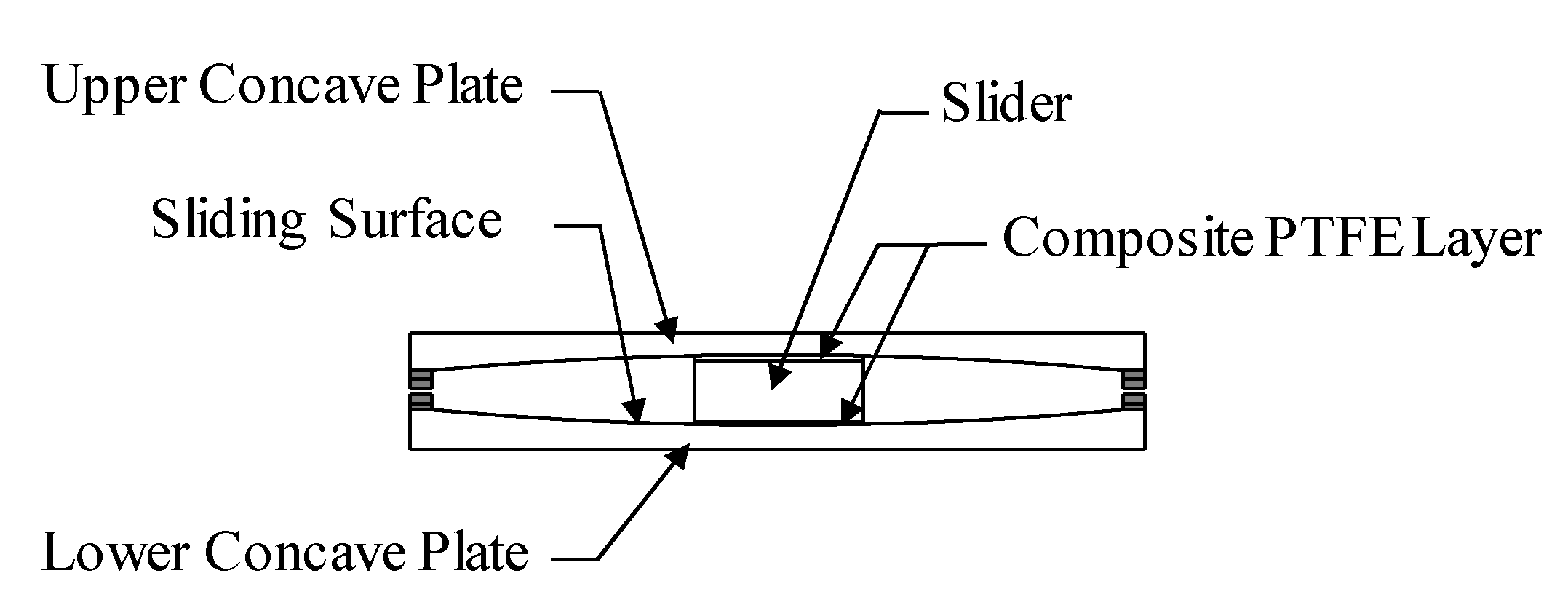
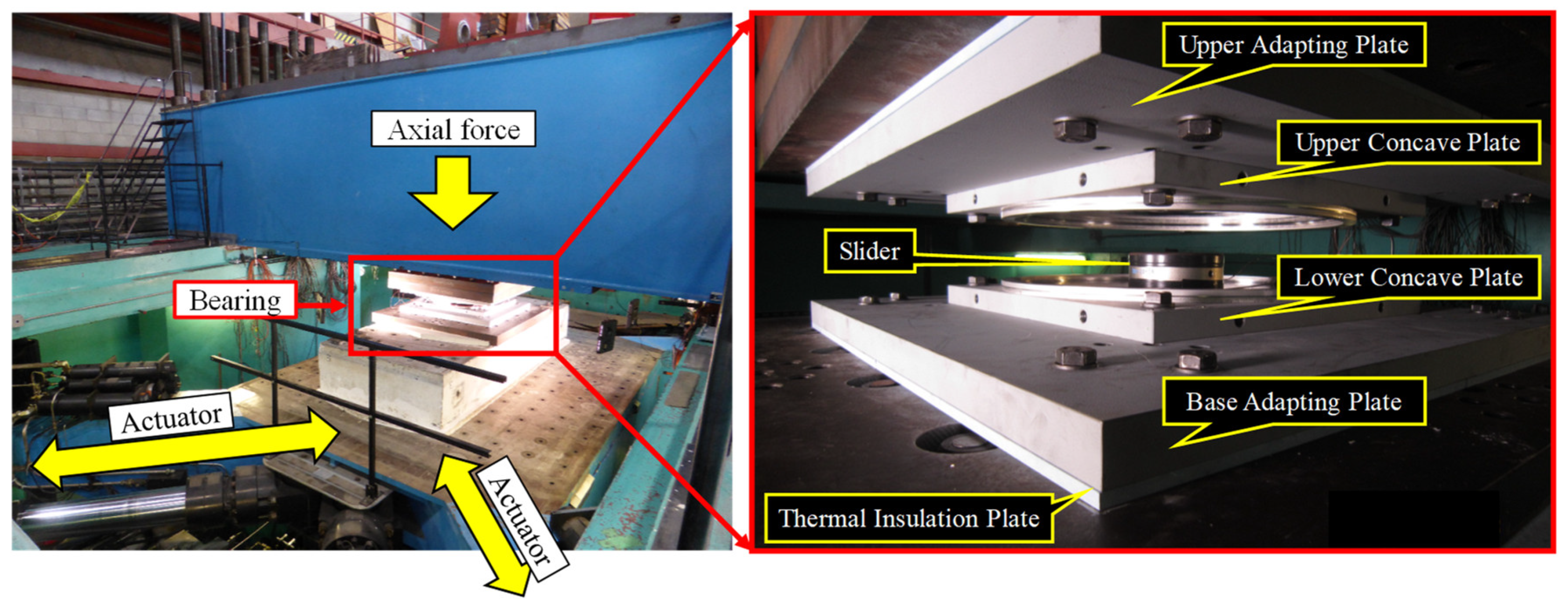
3.1. Testing Setup

The experiments in this study were conducted at the University of California, San Diego, in the Caltrans Seismic Response Modification Device (SRMD) Test Facility [13]. An overview of the test setup is shown in Figure 2. After the specimen was placed inside the facility, an axial force was added to control the contact pressure between the slider and the concave plate. Additionally, four horizontal actuators made the loading table move horizontally in order to control the velocity and loading path.

3.2. Dependency Tests

Pressure, velocity and temperature dependency equations were introduced in previous studies [14,15,16]. The applicability of the pressure and velocity dependency equations for specimens with slider diameters of 300 and 400 mm and spherical radii of the concave plates (R_s) of 4500 mm were verified under different pressures through the dependency test introduced in

Table 1. Test procedure of the dependency test.

Spec.	Test	Pressure	Amplitude	Vmax	Period	Cycle
num.	num.	N/mm2	±mm	mm/s	s	num.
φ300 φ400	(1) Velocity dependency test
	T01	60	200	400	3.14	4
	(2) Pressure dependency test
	T02	40	200	20	62.83	4
	T03	60		20	62.83	4
	T04	80		20	62.83	4

. The input waves were unidirectional sinusoidal displacement variations, and the amplitude, maximum velocity (Vmax), period and number of cycles were determined.

3.3. ASCE Tests

The dynamic tests shown in

Table 2. Test procedure of the ASCE test.

Spec.	Test	Pressure	Amplitude	Vmax	Period	Cycle
num.	num.	N\mm2	±mm	mm/s	s	num.
φ300 φ400	T01	60	268	392	4.26	3
	T02		10	14.646	4.26	20
	T03		100	146.369	4.26	3
	T04		200	292.738	4.26	3
	T05		268	392.269	4.26	3
	T06		400	585.476	4.26	3
	T07		400	585.476	4.26	3
	T08	40	400	585.476	4.26	3
	T09	80	400	585.476	4.26	3
	T10	30	440	644.024	4.26	1
	T11	90	440	644.024	4.26	1
	T12a	60	300	439.107	4.26	7
	T12b					7
	T12c					6
	T13		268	392.269	4.26	3

were conducted to validate the friction models under various situations. The test procedure was designed based on ASCE/SEI 7-16. Thus, it was named the ASCE test.

4. Numerical Simulation of the Experiments

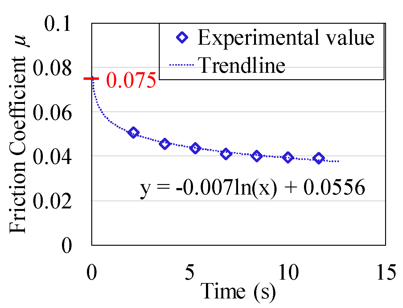
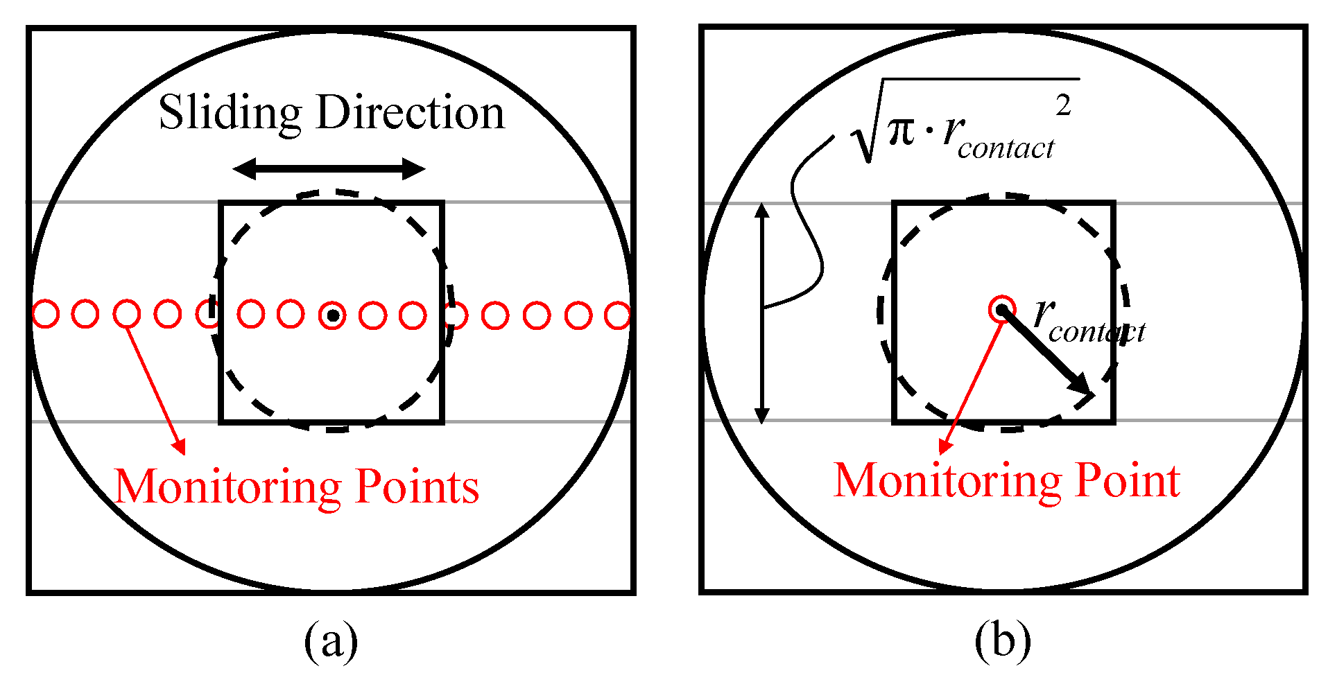
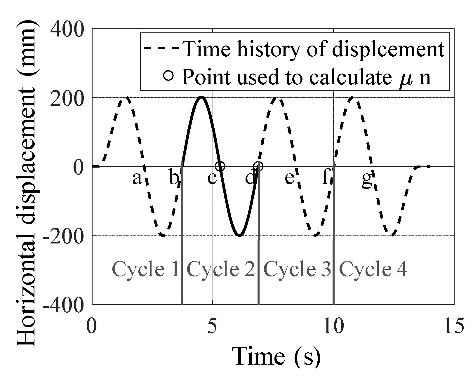
4.1. Friction Dependency

The pressure dependency of the friction coefficient could be considered by a pressure dependency factor γ, which is related to the bearing stress σ at the contact area of the concave plate and the slider. The pressure dependency equation was obtained by a previous experimental study [14]:

$$\gamma =2.03\times {\sigma }^{-0.19}+0.068$$

(7)

The dependency of the friction coefficient on velocity was considered by a velocity dependency factor α. This factor was related to the velocity of the upper concave plate relative to the lower concave plate v, which could be described by the following equation [14]:

$$\alpha =1-0.55\times e^{-0.019v}$$

(8)

Figure 3 shows the applicability verification of the pressure and velocity dependency equations for φ300 and φ400 specimens, based on the dependency test introduced in Table 1. In Figure 3, the experimental friction coefficients calculated from the dependency test were normalized by the values at 60 N/mm² and 400 mm/s, respectively, in order to minimize the influence of product variation. As a result, Equations (7) and (8) are both highly consistent with the experimental results, and thus, the previously proposed pressure and velocity dependency equations are effective for DCFP bearings with φ300 and φ400 slider diameters.

The temperature dependency equation is as follows:

$$\beta =1.13\times \exp (-0.007T)$$

(9)

where β is the temperature dependency factor and T is the temperature of the contact area between the slider and the concave plate in Celsius [15,16]. As the temperature, T, is difficult to accurately measure during testing, a numerical method proposed by Constantinou, M.C. et al. [4,17] will be introduced to simulate the temperature in the next section.

The friction coefficient at each time during excitation can be calculated by:

$$\mu ={\mu }_0\times \gamma \times \alpha \times \beta$$

(10)

where µ, γ, α and β are the friction coefficient, pressure dependency factor, velocity dependency factor and temperature dependency factor at each time, respectively, and µ_o is the friction coefficient at 60 N/mm² (γ = 1), 400 mm/s (α = 1) and an atmosphere temperature of around 20 °C (β = 1), which was selected as 0.075 for all the specimens in this study. µ_o was calculated from the trend line of the friction coefficient versus the time from the dependency test T01 in Table 1, which was when the time was approaching zero, as shown in Figure 4. The experimental values in this figure represent the friction coefficients near zero displacement where the velocity was 400 mm/s and the pressure was 60 N/mm².

4.2. Friction Models

Two friction models are proposed as precise and simplified models, and both considered the pressure, velocity and temperature dependency introduced in Section 4.1. Meanwhile, the precise model applies the precise temperature simulation model shown in Figure 5a and the simplified model applies the simplified temperature simulation model shown in Figure 5b, where r_contact is the radius of the bearing and the monitor points are virtual points in the model used for temperature simulation, which is proposed by Constantinou, M.C. et al. [4,17]. As the precise model has a lot of monitoring points along the sliding direction, the simulation results are more precise. However, for the simplified model, which only applies one monitoring point, the calculation speed is much faster. Therefore, the validation of the simplified model is very important in judging whether it can be used instead of the precise model.

In both the precise model and the simplified model, the temperature increase of the monitoring points can be calculated by [17]:

$$\Delta T(t)=\frac{\sqrt{D}}{k\sqrt{\pi }}{{\displaystyle \int }}_0^t\frac{q(t-\tau )d\tau }{\sqrt{\tau }}$$

(11)

where q(t) is the heat flux at the surface of the solid; ΔT(t) is the temperature increase at time t, compared to the temperature at t = 0; τ is a time parameter that varies between 0 and t; D is the thermal diffusivity of the solid; and k is the thermal conductivity of the solid [17]. In this study, the values of k and D were adopted from the “JSME Data Book: Heat Transfer”, which are 0.016 W/(mm∙°C) and 4.07 mm²/s, respectively [18]. Then the temperature at the contact surface of the slider and the concave plates can be calculated by taking average of the temperature of the monitoring points within the contact surface.

For DCFP Bearings, the instantaneous heat flux, q(t), can be defined as follows [4]:

$$q(t)=\{\begin{array}{c}\mu (t)p(t)\frac{v(t)}{2} \mathrm{if} \delta \le \sqrt{\pi \cdot r_{contact}{}^2}/2\\ 0\mathrm{otherwise}\end{array}$$

(12)

where μ(t), p(t) and v(t) are the coefficient of friction, the pressure at the contact area and the relative velocity between the upper and lower concave plates at time t, respectively; δ is the lateral distance from the center of the slider to the monitor point of interest and r_contact is the contact radius.

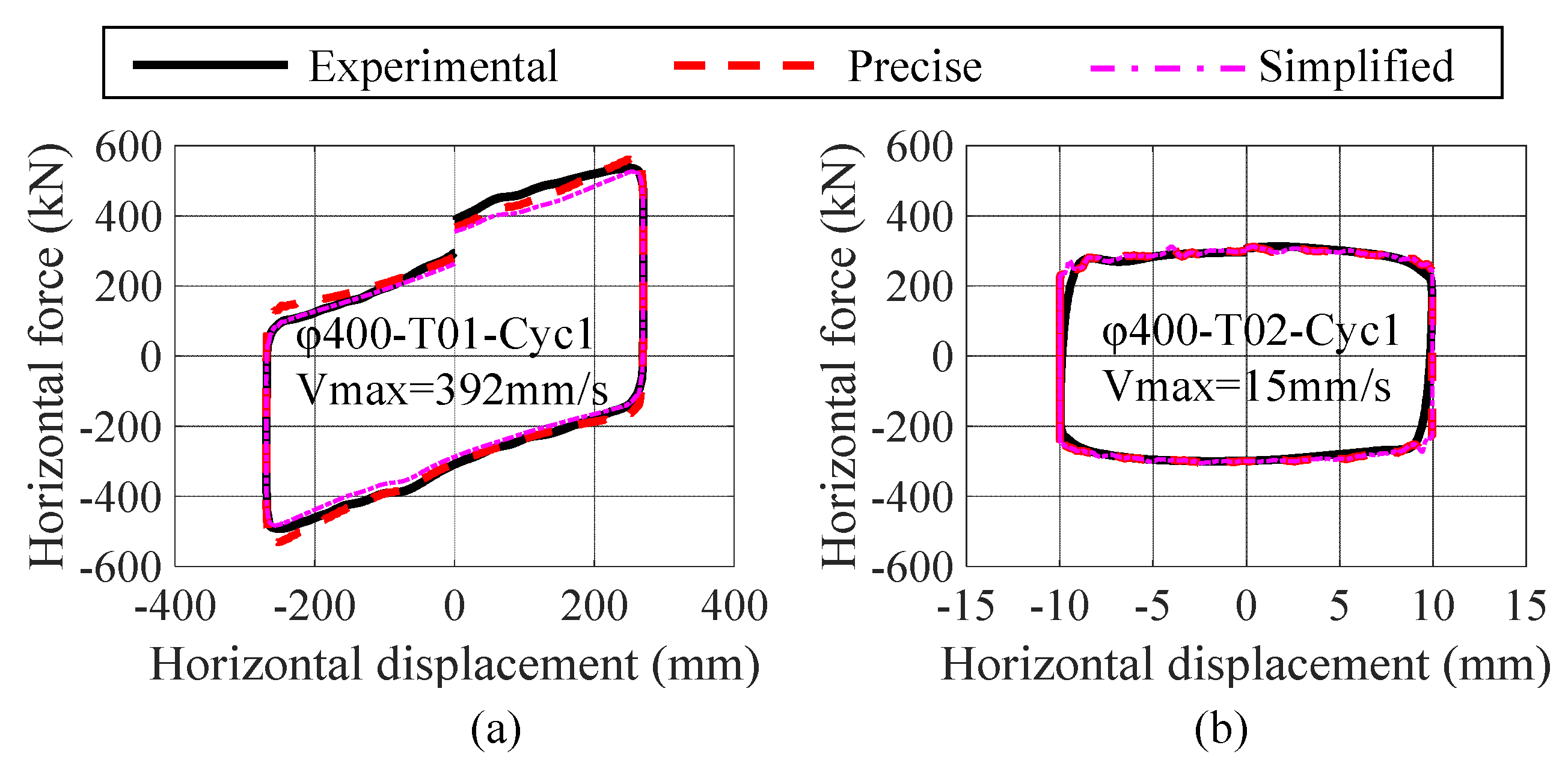
4.3. Numerical Results Using Friction Models

The comparison of the first hysteresis curve between the friction models and the experimental results of the DCFP bearings with 400 mm-diameter sliders under both strong and weak excitations are shown in Figure 6, and show high accuracy for both friction models. The input excitations in Figure 6a,b are the first cycles in T01 and T02 of the ASCE test, respectively. Meanwhile, as an error criterion, the values of the post-yield stiffness, effective stiffness, effective damping and energy dissipated per cycle were also calculated to quantify the validity of the models [6]. In all of the ASCE tests, the simplified model shows a similar accuracy to the precise model, with both models showing high accuracy in the simulation of the behaviours of the DCFP bearings [19].

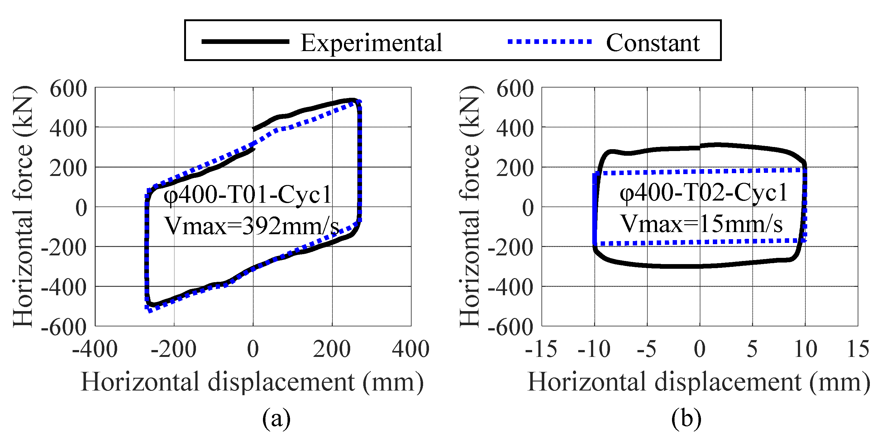
4.4. Numerical Results Using a Constant Friction Coefficient

In order to find the constant friction coefficient that was suitable for the most amount of time during most seismic situations, a nominal friction coefficient, µ_n, was defined. The value of µ_n was 0.043 for both sizes of the sliders based on experimental results, and it represented the nominal friction coefficient under seismic load conditions. This value was determined by taking the average of the friction coefficient of the DCFPB at zero displacement points in the second cycle (points c and d in Figure 7) of the input sine wave with a constant pressure of 60 N/mm² and a maximum velocity of 400 mm/s (T01 of the dependency test in Table 1).

The accuracy of using µ_n under strong excitation and weak excitation is shown in Figure 8. The results showed that µ_n was suitable for strong excitations but could not be used under weak excitations. In the other tests in Table 2, which can all be considered to be strong excitations, the simulations using µ_n all showed that the force–deflection relations of the DCFP bearings had no large differences [19]. Therefore, the constant friction coefficient, µ_n, could be applied for the rough behavior estimation of DCFP bearings under seismic loads. For example, it could be applied for the response force simulation when the response displacement of the bearing is known.

In the numerical simulation of DCFP bearings, pressure, velocity and temperature dependencies all have influence on the behavior of the bearings. However, for DCFP bearings under stable pressure, the temperature variation caused by friction heating will dominate the influence. This influence is more obvious when the temperature is relatively low (e.g., 20–100 °C), meaning that it is under weak excitations, as shown in Figure 6b and Figure 8b. However, when the temperature is higher, the influence will ease up, as shown in Figure 6a and Figure 8a, and this is the reason why the constant friction coefficient can be applied for rough estimation under strong excitations such as seismic loads.

5. Numerical Analyses of the Dynamic Response of Isolated Structures

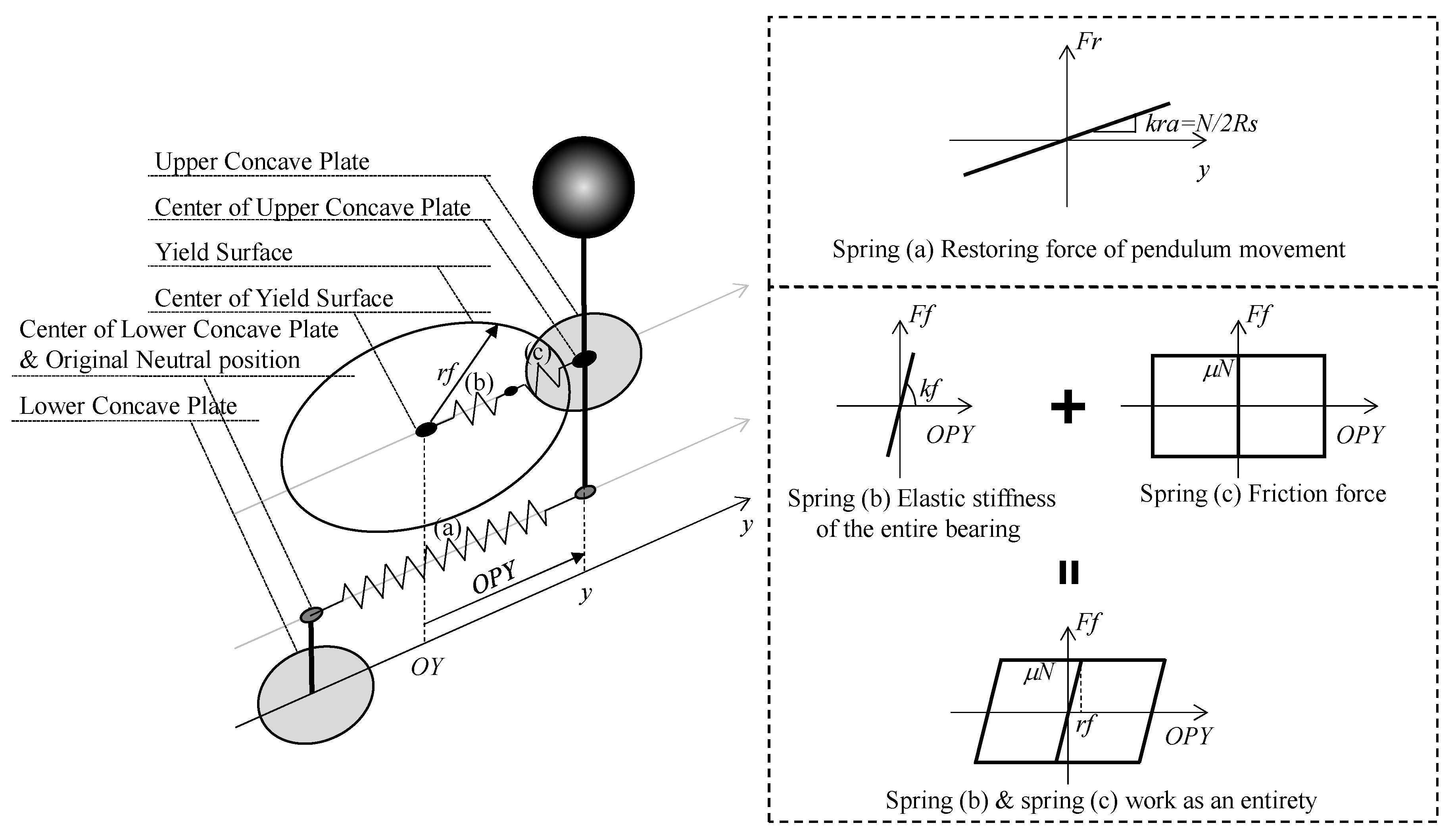
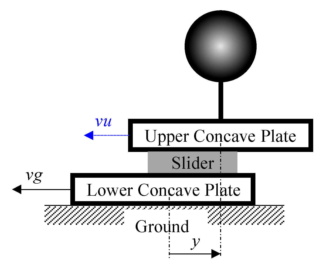
5.1. Mechanical Model

The mechanical model used in this study is shown in Figure 9 and considered both static and dynamic friction [20]. To demonstrate the relation of the response of the isolation layer and the earthquake records more clearly, the upper structure is set as a rigid body.

In Figure 9, the center of the lower concave plate is taken as the original neutral position. The stiffness of the upper structure is considered to be infinite in order to make the behavior of the DCFP bearing clearer. Whether sliding between the slider and the concave plate will occur or not is considered by a yield surface with a radius r_f [21,22]. OY is the center of the yield surface, y is the displacement of the upper structure relative to the center of the lower concave plate and OPY is the distance from OY to y. The internal forces of the DCFP bearing are considered in terms of three springs: spring (a), spring (b) and spring (c). Spring (a) represents the restoring force of the pendulum movement. k_ra is the stiffness, N is the vertical force that acts on the DCFP bearing, and R_s is the spherical radius of the upper and lower concave plates. In this study, the DCFP bearings with slider diameters equal to 400 mm and R_s values equal to 4500 mm are set, and a vertical load that can provide 60 MPa of pressure on the slider surface is applied. Therefore, k_ra equals 0.838 kN/mm. Spring (b) represents the elastic stiffness of the entire DCFP bearing with a value of k_f = 1900 kN/mm, based on experimental results. Spring (c) represents the friction force between the slider and two concave plates. Spring (b) and spring (c) work entirely to simulate the friction force. The friction force is represented by spring (b) when there is no sliding and by the friction models, introduced in Section 2, during sliding.

5.2. Input Ground Motions

In order to see whether the simplified model could be used instead of the precise model in the response analysis and later as the analysis database for the prediction method, the earthquake inputs shown in

Table 3. Input earthquake motion.

Abv.	Earthquake	Station	PGV (m/s)	Duration (s)	Field
JKB	Kobe	JMA Kobe	0.893	30	Far
KNA	Kobe	Nishi-Akashi	0.373	41	Near
TC1	Chi-Chi	TCU129	0.554	90	Near
NCC	Northridge	Canyon Country-WLC	0.449	20	Far
LPG	Loma Prieta	Gilroy Array	0.447	40	Near
IVD	Imperial Valley	Delta	0.330	100	Near
TSD	Tohoku	JMA Sendai	0.545	180	Near
TIM	Tohoku	JMA Ishinomaki	0.376	300	Near

were selected. These inputs include earthquake records with various intensities, various durations and both near and far fields. Additionally, in order to study the behavior of the isolation system under earthquakes with similar intensities, each earthquake record was amplified to four input waves with PGVs (Peak Ground Velocities) equal to 0.25, 0.50, 0.75 and 1.00 m/s. In Table 3, the first column shows the abbreviation of the earthquake record, which is consist of the name and the measuring station of the earthquake.

5.3. Accuracy of the Simplified Model

As shown in Figure 10, the response analysis results using the simplified model were as good as those using the precise model under both strong and weak earthquake excitations. This was because, in both cases, the slider was on the monitoring point of the simplified model for most of time. In the response analysis of all the other input waves introduced in Table 3, the response analysis results using the simplified model could always provide results with similar accuracy to those obtained using the precise model. Thus, the simplified model was used in the response analysis instead of the precise model in order to save time.

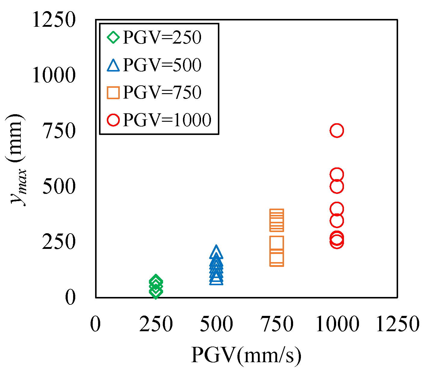
5.4. Relation between Maximum Response Displacement and PGV

Based on the simulation results, the relationship between the maximum response displacement of the isolation layer (y_max, which is the maximum relative displacement between the upper concave plate and the lower concave plate) and the peak ground velocity (PGV) of the input earthquake is shown in Figure 11. It can be seen that, even though they have the same PGV, different earthquake inputs can still cause different y_max. The difference may be caused by other earthquake characteristics such as the ground acceleration and the bearing’s friction coefficient during excitation. These factors are also related to the transfer of the input energy in the isolation layer. The relationship between them will be studied in the next chapter.

6. Proposed Prediction Method

A simple method is proposed in this chapter to predict the response of an isolation system under a certain unidirectional earthquake input and the energy transfer during a process based solely on the earthquake record. Furthermore, the method was simplified and optimized based on the response analysis results. Finally, how this method could be applied to general design factors was also studied.

6.1. Mechanical Model

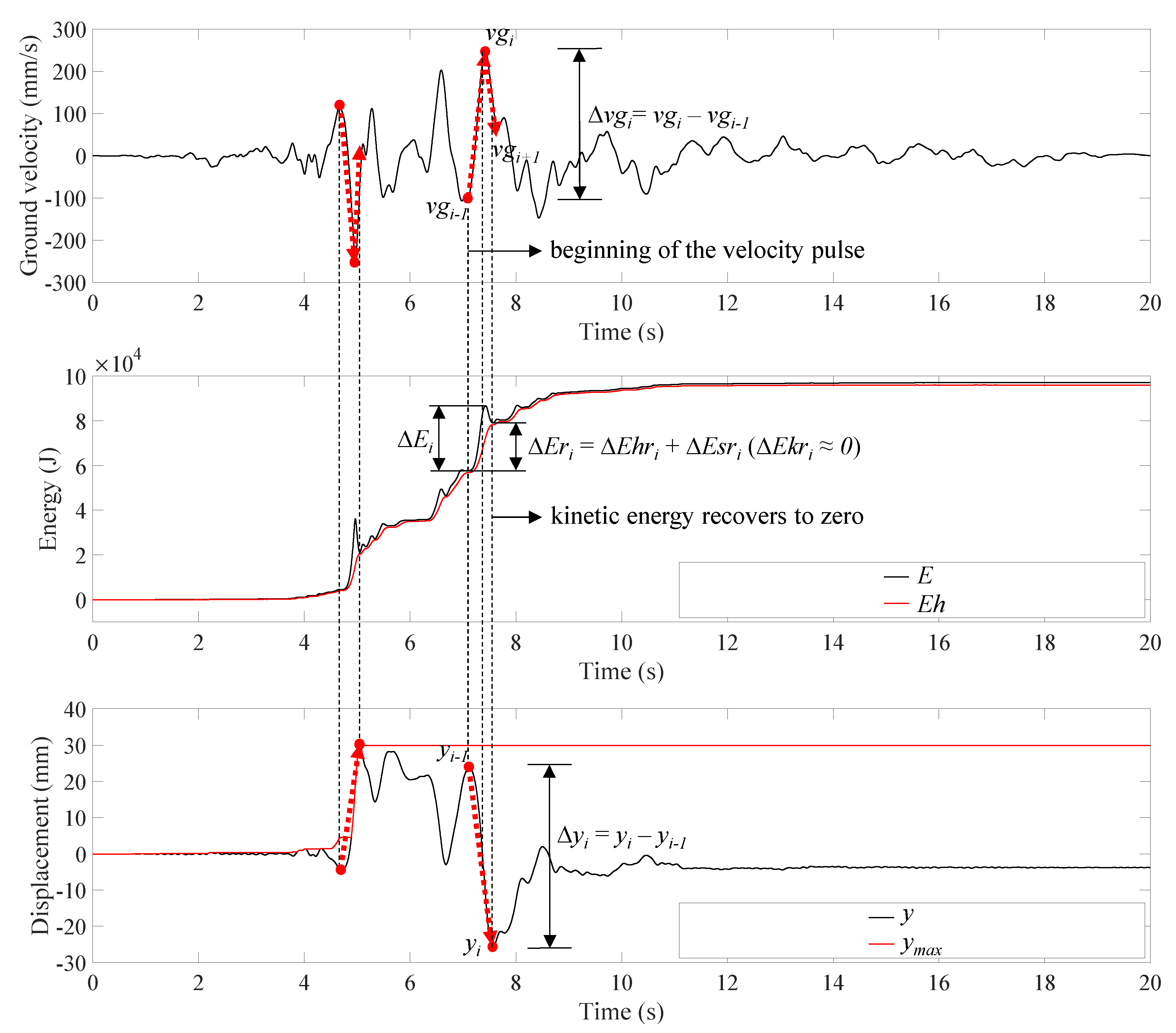
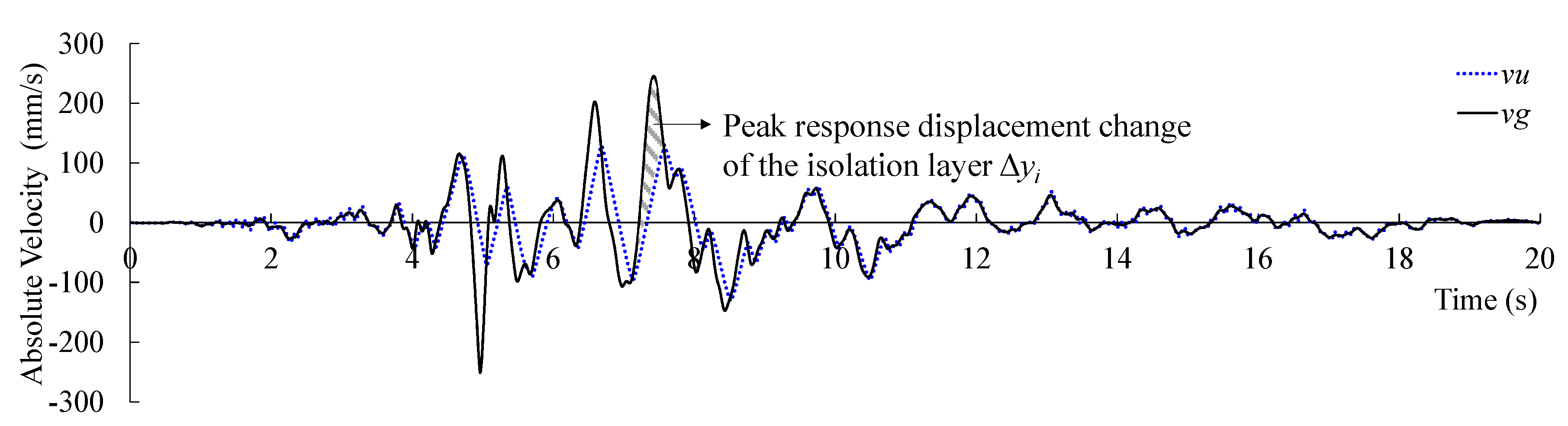
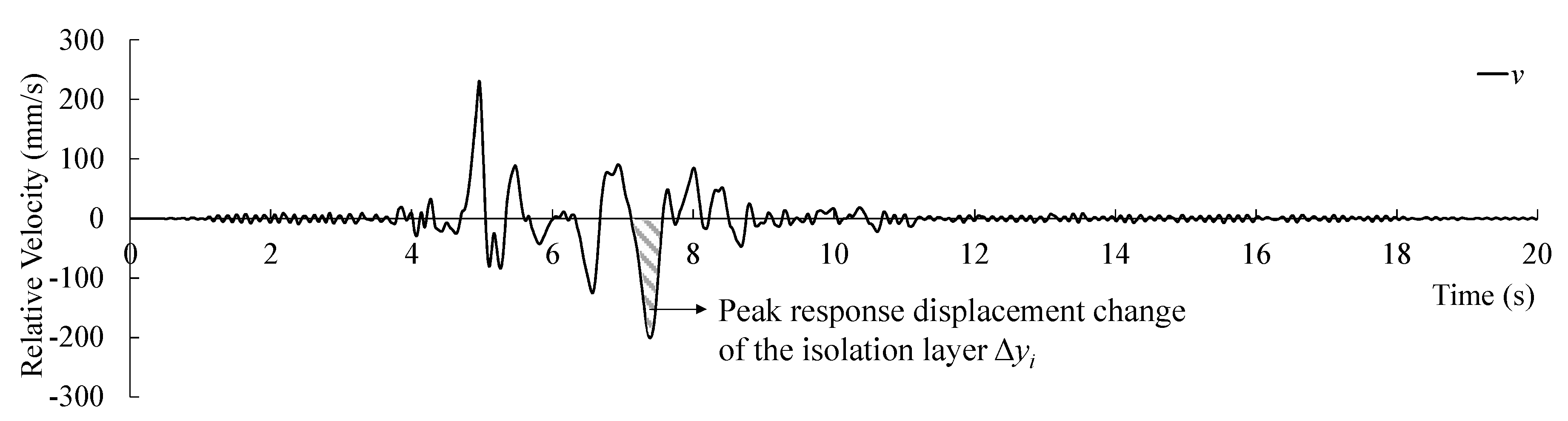
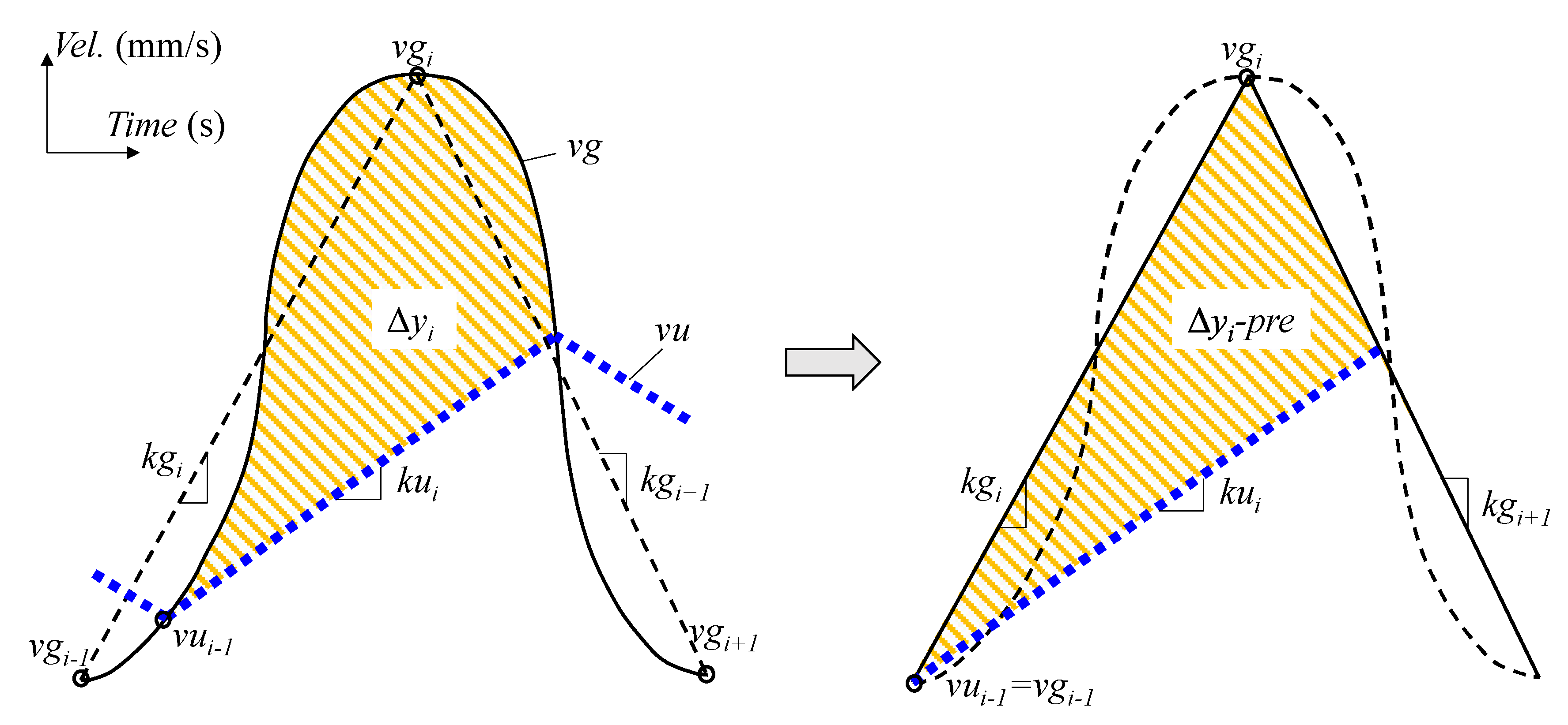
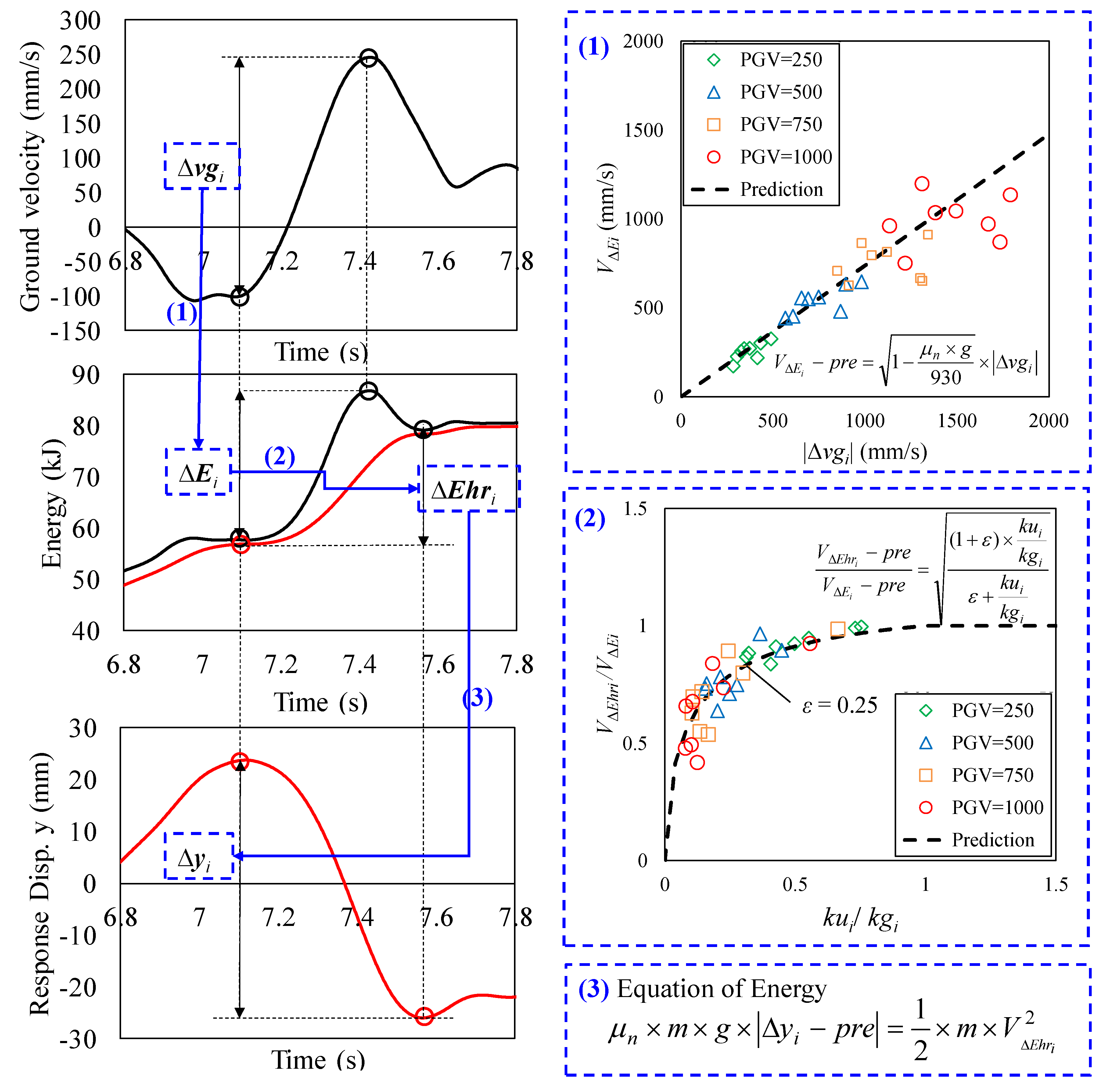
6.1.1. Relationship between Ground Velocity, the Response Displacement and the Input Energy of the Isolation Layer.

By using the model in Figure 9, the relative movement and the energy balance in a base-isolated building become the relative movement and the energy balance in the base-isolated layer.

As one matter of concern during the design stage, the prediction of the maximum relative displacement between the upper and lower concave plates of the bearing during earthquakes is the focus of this study. Figure 12 shows the relative movement of the base-isolated layer during strong earthquake pulses, where vu is the absolute velocity of the upper structure, vg is the absolute velocity of the ground, and y shows the relative displacement between the upper and lower concave plates, which can also be called the response displacement of the isolation layer. Then, the response velocity of the isolation layer (the relative velocity between the upper and lower concave plates) can be expressed as:

$$v=\dot{y}=vu-vg$$

(13)

During a strong earthquake pulse, the history of vg is known and the value of vu is mainly determined by the dynamic friction coefficient of the bearing. Therefore, y can be predicted by integral v, which is the difference between vu and vg.

Based on the response analysis results, the ground velocity record of the earthquake was found to be greatly related to, and work simultaneously with, the transferred energy and the response displacement of the isolation layer during earthquakes. As shown in Figure 13, during one earthquake, several large velocity pulses (from one ground peak velocity, vg_i−1, to the next peak, vg_i, and to the next peak, vg_i+1, is one velocity pulse) exist. The difference between vg_i−1 and vg_i was defined as the velocity difference of this velocity pulse, Δvg_i, which could show the intensity of the velocity pulse:

$$\Delta v{g}_i=v{g}_i-v{g}_{i-1}$$

(14)

It was found that, when a large Δvg_i exists in the earthquake, it will lead to large input energy in the structural system, ΔE_i, and a large response displacement of the isolation layer (a large relative displacement between the upper concave plate and the lower concave plate), Δy_i, simultaneously. Since the upper structure is considered to be a rigid body in this study, the total input energy, E, is consumed by the hysteresis energy E_h. However, during a velocity pulse, some of the input energy will first be temporarily stored in the kinetic energy, E_k, and the elastic strain energy, E_s. In order to eliminate the interference of E_k, the change in energy from the beginning of the velocity pulse to the time kinetic energy recovers to zero, which is approximately the time interval from y_i−1 to y_i and is considered to be very useful as it is related to the peak response displacement change, Δy_i. In Figure 13, y_i and y_i−1 are two neighboring peak response displacements of the isolation layer, and every time a peak response displacement is achieved, E_k becomes zero; y_max is the maximum amplitude of the response displacement of the isolation layer; Δy_i is one of the peak response displacement changes of the isolation layer, and the one shown in the figure is the maximum. Then, in this time interval, the total input energy, ΔEr_i, can be expressed as the sum of the consumed energy. ΔEhr_i and the change in the elastic strain energy, ΔEsr_i, with the change in kinetic energy, ΔEkr_i, were also considered to be zero:

$$\Delta E{r}_i=\Delta Eh{r}_i+\Delta Es{r}_i\begin{array}{cc}& (\Delta Ek{r}_i=0)\end{array}$$

(15)

Since the elastic strain energy was also relatively small in this study, the value of it could be ignored under large velocity pulses. Then, ΔEr_i in this time interval can be expressed as:

$$\Delta E{r}_i=\Delta Eh{r}_i$$

(16)

To see exactly how the ground velocity record determines the response displacement of the isolation layer, the velocity history of the upper structure, vu, and the ground, vg, based on the response analysis, is shown in Figure 14, where, based on Equation (13), the area between the velocity history of the upper structure and the ground is the response displacement of the isolation layer. It can be seen from the time history of vu that the acceleration of the upper structure during large velocity pulses is roughly constant. Therefore, in the prediction, it is reasonable to consider the friction coefficient during large velocity pulses to be constant.

In Figure 15, the same response displacement is shown in the time history of the response velocity of the isolation layer, v.

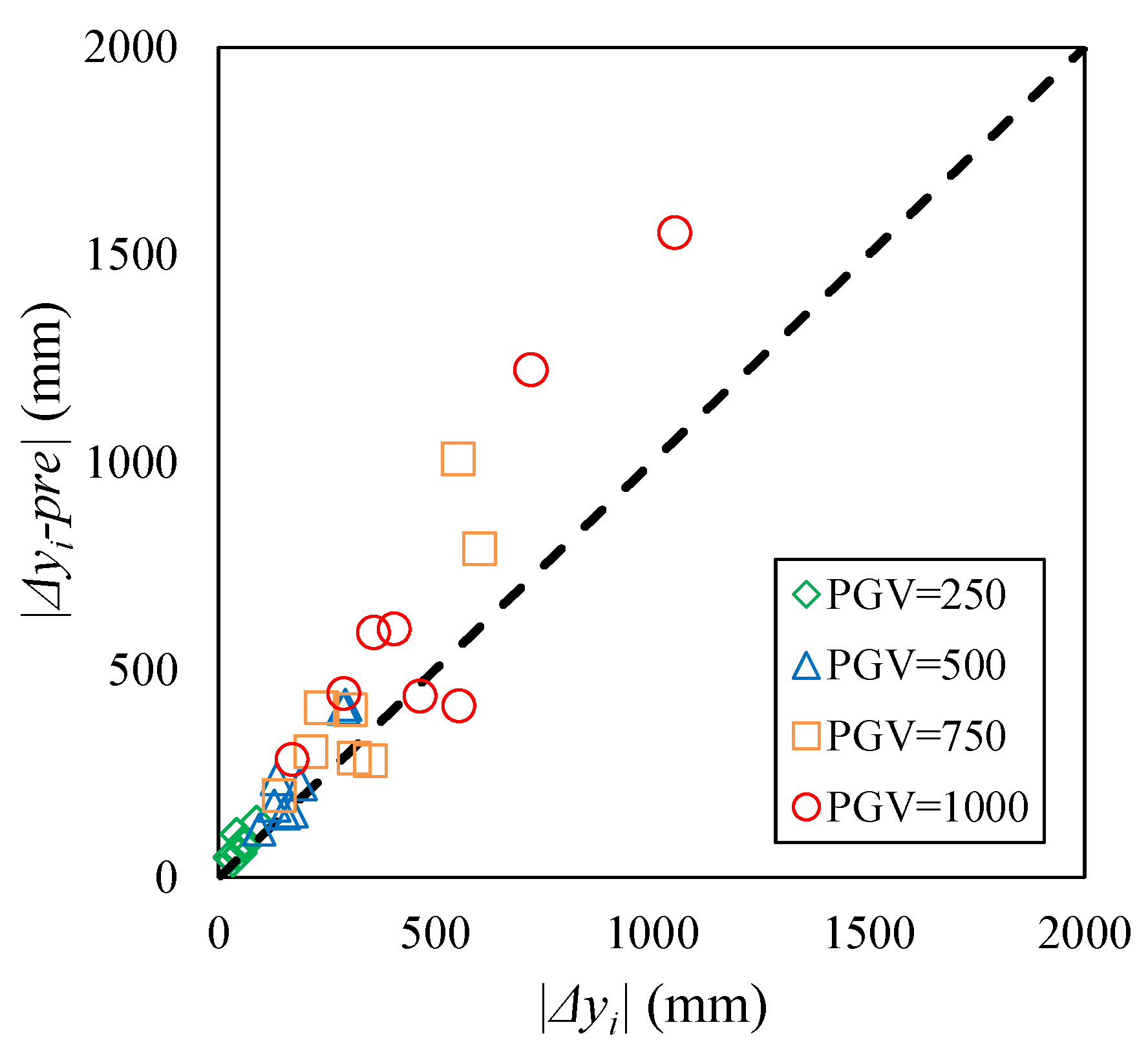
6.1.2. Prediction of the Response Displacement of the Isolation Layer

In this section, the peak response displacement changes in the isolation layer, Δy_i, were primarily predicted by simplifying Figure 14. It should be mentioned that Δy_i was predicted instead of y_max. This was because the value of y_max was highly related to former response displacement, which made it difficult to be derived theoretically. However, the derivation of Δy_i was more related to the corresponding velocity pulse. Furthermore, since the maximum Δy_i was usually larger than y_max, the maximum Δy_i could be considered to be a conservative value of y_max.

As shown in the left figure of Figure 16, the solid line shows a ground velocity pulse from vg_i−1 to vg_i to vg_i+1 and the two dashed lines show the slope from vg_i−1 to vg_i and the slope from vg_i to vg_i+1, respectively, which can be understood as the average ground acceleration. The dotted line is the absolute velocity of the upper structure, and its slope can be roughly considered to be constant, as introduced in Figure 14. Furthermore, since the points where vu and vg intersect are determined by the former velocity history, the intersection in the left figure of Figure 16 was randomly picked between vg_i−1 and vg_i, referred to as vu_i−1. At the intersection points, vu was equal to vg, which meant that v was equal to zero, and this meant that the direction of the response displacement of the isolation layer, y, would change from the next second. Then, until the next intersection, y would be in the same direction; reach the peak displacement change, Δy_i; and reverse direction again. Then, how the calculation of Δy_i can be simplified under a large velocity pulse is shown in the right figure of Figure 16. In the simplification, vu_i−1 and vg_i−1 are assumed to be equal, which is a conservative assumption for predicting Δy_i:

$$v{u}_{i-1}=v{g}_{i-1}$$

(17)

The acceleration between two adjacent peak ground velocities is assumed to be the average value, kg_i and kg_i+1:

$$\begin{array}{cc}k{g}_i=\frac{v{g}_i-v{g}_{i-1}}{\Delta t_i};& k{g}_{i+1}=\frac{v{g}_{i+1}-v{g}_i}{\Delta t_{i+1}}\end{array}$$

(18)

where Δt_i is the time interval between vg_i−1 and vg_i; Δt_i+1 is the time interval between vg_i and vg_i+1.

The friction coefficient was assumed to be the nominal friction coefficient, μ_n, which was equal to 0.043 and could be used to roughly simulate the behavior of the bearing under earthquake excitations. Therefore,

$$k{u}_i={\mu }_n\times g\times k{g}_i/\left|k{g}_i\right|$$

(19)

where g is the gravity acceleration in mm/s².

Then, the predicted value will be Δy_i-pre, as shown in Figure 16, which is the predicted peak response displacement of the isolation layer.

It can be seen from Figure 16 that, when the value of ku_i is close to kg_i, Δy_i-pre is close to zero. However, based on the response analysis results, Δy_i can also be relatively large in this situation. Therefore, a special prediction method was proposed for these cases, as shown in Figure 17, in which the case of ku_i/kg_i being equal to 1.0 is shown. Based on the response analysis results, the cases of ku_i/kg_i being between 0.8 and 1 should use this method and the cases of ku_i/kg_i being between 0 and 0.8 should use the method in Figure 16.

Therefore, as shown in the right half of Figure 16, for the cases of ku_i/kg_i being between 0 and 0.8, Δy_i-pre (the predicted value of the peak response displacement change of the isolation layer) can be predicted by vg_i-1, vg_i, kg_i, kg_i+1 and ku_i, which are given by the time history data of the earthquake record and Equation (19).

$$\begin{array}{ll}\Delta y_i-pre& =-\frac{1}{2}\times (k{g}_i-k{u}_i)\times {(\frac{v{g}_i-v{g}_{i-1}}{k{g}_i})}^2\times (1+\frac{k{g}_i-k{u}_i}{k{u}_i-k{g}_{i+1}})\\ & =-\frac{(k{g}_i-k{u}_i)\times (k{g}_i-k{g}_{i+1})}{2\times k{g}_i^2\times (k{u}_i-k{g}_{i+1})}\times {(v{g}_i-v{g}_{i-1})}^2\end{array}$$

(20)

As for the cases of ku_i/kg_i being between 0.8 and 1, the value of vg_i−1, vg_i, kg_i and kg_i+1 should be amplified by 1.5 before using Equation (20).

The accuracy was between 1 and 2.1, as shown in Figure 18, which is a conservative prediction with an error caused by the assumptions shown in Equations (17)–(19).

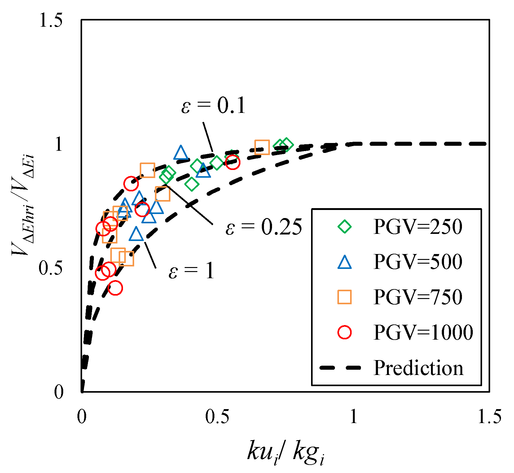
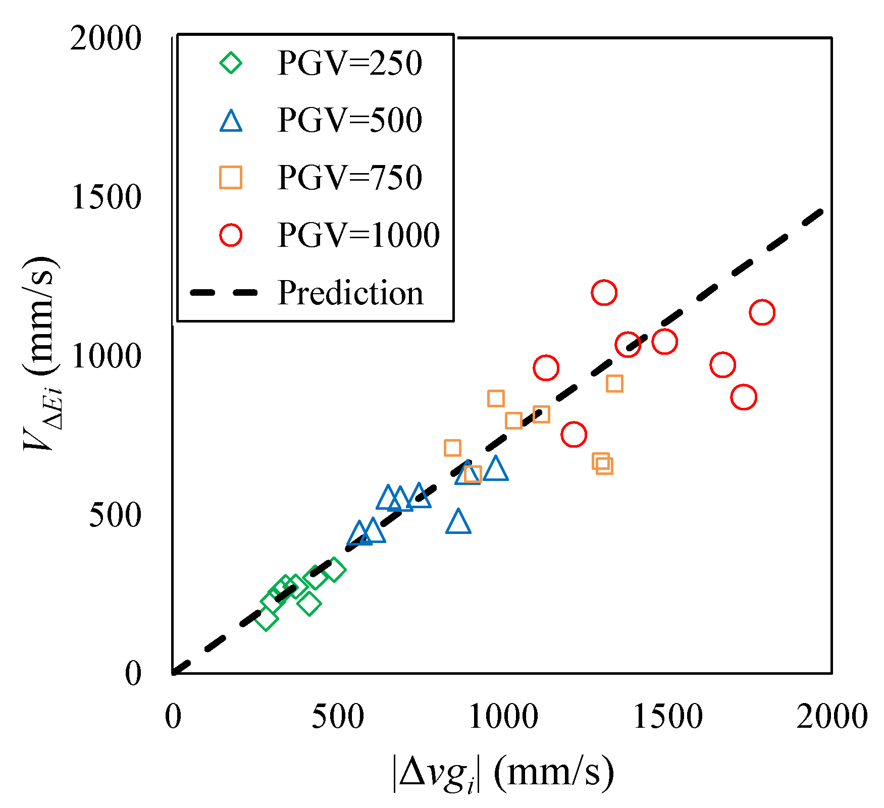
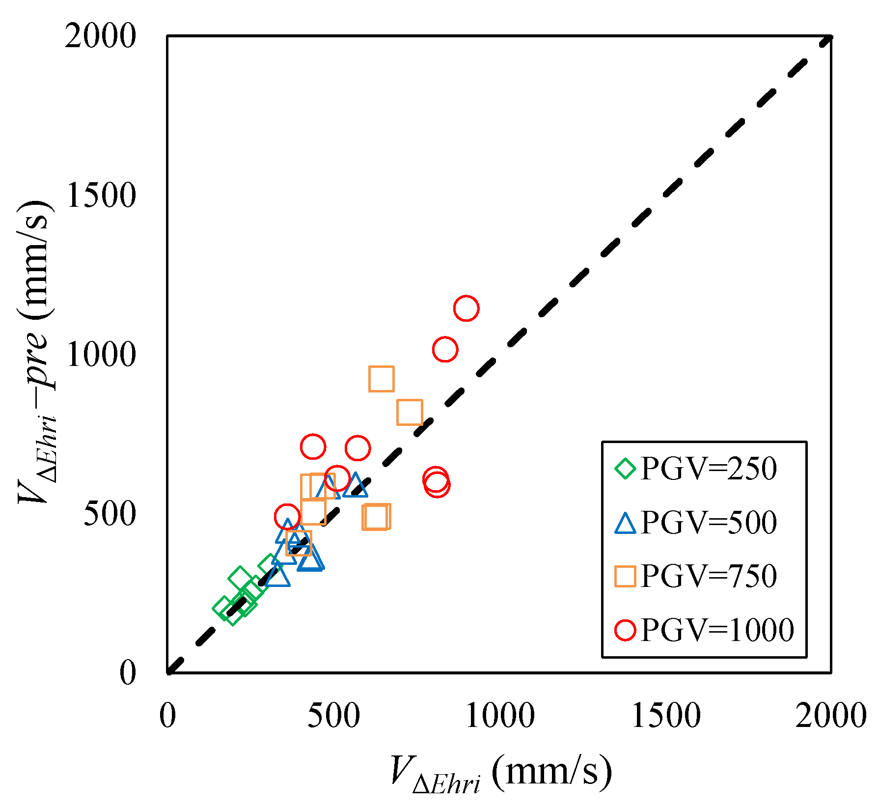
6.1.3. Prediction of Energy Transfer

The input energy of the isolation layer was defined by Equation (4) in the introduction. Since the response displacement of the isolation layer, y, can be predicted, the total input energy to the isolation layer between vg_i−1 and vg_i can also be predicted by vg_i-1, vg_i, kg_i, kg_i+1 and ku_i, which were given by time history data of the earthquake records and Equation (19):

$$\begin{array}{ll}\Delta E_i-pre& =m\times k{g}_i\times \frac{1}{2}\times (k{g}_i-k{u}_i)\times {(\frac{v{g}_i-v{g}_{i-1}}{k{g}_i})}^2\\ & =\frac{1}{2}\times m\times (1-\frac{k{u}_i}{k{g}_i})\times {(v{g}_i-v{g}_{i-1})}^2\end{array}$$

(21)

The equivalent velocity [9] of the total input energy is:

$$V_{\Delta E_i}-pre=\sqrt{1-\frac{k{u}_i}{k{g}_i}}\times \left|v{g}_i-v{g}_{i-1}\right|$$

(22)

The amount of ΔE_i consumed by the hysteresis energy, ΔE_i, can be predicted by vg_i−1, vg_i, kg_i, kg_i+1 and ku_i, which were given by the time history data of the earthquake records and Equation (19):

$$\begin{array}{ll}\Delta Eh{r}_i-pre& =m\times k{u}_i\times \Delta y_i-pre\\ & =\Delta E_i-pre\times \frac{k{u}_i\times (k{g}_i-k{g}_{i+1})}{k{g}_i\times (k{u}_i-k{g}_{i+1})}\end{array}$$

(23)

The equivalent velocity of the consumed energy is:

$$V_{\Delta Eh{r}_i}-pre=\sqrt{1-\frac{k{u}_i}{k{g}_i}}\times \left|v{g}_i-v{g}_{i-1}\right|\times \sqrt{\frac{k{u}_i\times (k{g}_i-k{g}_{i+1})}{k{g}_i\times (k{u}_i-k{g}_{i+1})}}$$

(24)

The accuracy of V_ΔEi-pre was between 0.8 and 1.9, and the accuracy of V_ΔEhi-pre was between 0.8 and 1.6. It can be seen that this prediction method is relatively conservative.

6.2. Simplification and Optimization of the Prediction Method Based on the Analysis Results

6.2.1. Simplification of kg_i+1

By combining Equations (21) and (23), Equation (20) can be expressed in the form of energy as:

$$m\times k{u}_i\times \Delta y_i-pre=\frac{1}{2}\times m\times (1-\frac{k{u}_i}{k{g}_i})\times {(v{g}_i-v{g}_{i-1})}^2\times \frac{k{u}_i\times (k{g}_i-k{g}_{i+1})}{k{g}_i\times (k{u}_i-k{g}_{i+1})}$$

(25)

kg_i+1 was only contained in the rightmost fraction of Equation (25), which can be considered as the percentage of energy absorption, and it was attempted to simplify this fraction in order to not only simplify the equation but also make the method easier to apply in the design stage. Therefore, it is generalized with a generalization parameter, ε:

$$k{g}_{i+1}=-\epsilon \times k{g}_i$$

(26)

Then, the predicted percentage of the absorption can be expressed, in the form of equivalent velocity of energy, as:

$$\frac{V_{\Delta Eh{r}_i}-pre}{V_{\Delta E_i}-pre}=\sqrt{\frac{k{u}_i\times (k{g}_i-k{g}_{i+1})}{k{g}_i\times (k{u}_i-k{g}_{i+1})}}=\sqrt{\frac{(1+\epsilon )\times \frac{k{u}_i}{k{g}_i}}{\epsilon +\frac{k{u}_i}{k{g}_i}}}$$

(27)

By comparing the prediction value of Equation (27) to the analysis result points, as shown in Figure 19, 0.25 is considered to be the most suitable value of ε for the general calculation. It should be mentioned that, since the percentage of absorption will not exceed one, the value of V_ΔEhri-pre/V_ΔEi-pre can be taken as one when ku_i/kg_i is larger than one.

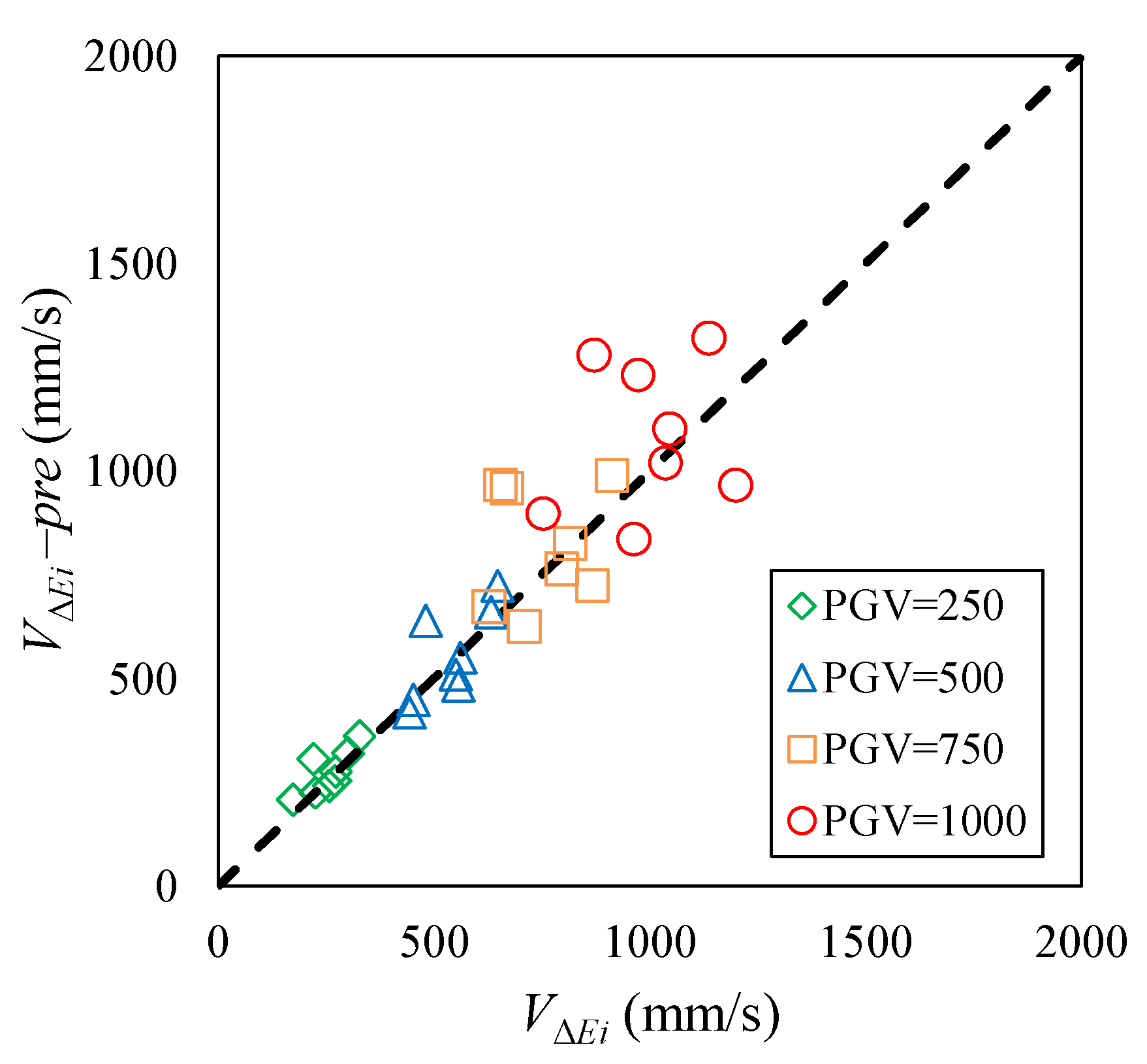
6.2.2. Simplification of the Prediction Equation of V_ΔEi-pre

Equation (22) gives the prediction equation of V_ΔEi-pre. It shows a linear relationship between V_ΔEi-pre and the absolute value of the peak ground velocity difference, |Δvg_i|, which equals to |vg_i- vg_i-1|. By observing the relationship between the analysis results for V_ΔEi and |Δvg_i|, as shown in Figure 20, it was found that the value of kg_i could be taken as a constant without causing large differences.

Therefore, the slope of the prediction line, based on Equation (22), is determined as:

$$\frac{V_{\Delta E_i}-pre}{\left|\Delta v{g}_i\right|}=\sqrt{1-\frac{k{u}_i}{k{g}_i}}\approx \sqrt{1-\frac{k{u}_i}{k{g}_{ave}}}=\sqrt{1-\frac{\left|k{u}_i\right|}{930}}$$

(28)

where the kg_ave = average value of kg_i (the kg_i corresponding to the maximum response displacement of the isolation layer) of the eight selected earthquakes with the PGV amplified as 250 mm/s², which was 930 mm/s². The value 930 mm/s² can be considered to be a constant value that can be used in most cases where the input earthquakes have PGVs larger than 250 mm/s², because the eight earthquakes selected in this study were considered to be representative.

6.2.3. Simplified and Optimized Prediction Method

By applying Equations (27) and (28), the proposed prediction method can be simplified, as shown in Figure 21.

The accuracies of V_ΔEi-pre, V_ΔEhri-pre and Δy_i-pre when using this simplified prediction method are shown in Figure 22, Figure 23 and Figure 24, respectively. The accuracy of V_ΔEi-pre was between 0.8 and 1.5, the accuracy of V_ΔEhri-pre was between 0.7 and 1.6, and the accuracy of Δy_i-pre was between 0.7 and 1.8.

6.3. Application of the Prediction Method in Design

In order to give a general prediction of the maximum response displacement change and input energy of an isolation layer under a group of earthquakes with a certain intensity, the specific earthquake characteristics, such as Δvg_i and kg_i, should be replaced. Therefore, Equation (29) is proposed, where ζ is the generalization parameter of the ground velocity. As shown in Figure 25, based on the earthquake records, |Δvg_i| was assumed to be 1.5 times the peak ground velocity (PGV) in this study.

$$\left|\Delta v{g}_i\right|=\varsigma \times PGV$$

(29)

kg_i was assumed based on the average value of kg_i of the eight selected earthquakes with PGVs amplified to 250 mm/s, which was 930 mm/s:

$$k{g}_i=930\times \frac{PGV}{250}$$

(30)

Therefore, the prediction method can be generalized as:

$$V_{\Delta E_i}-pre=\sqrt{1-\frac{{\mu }_n\times g}{930}}\times \varsigma \times PGV$$

(31)

$$V_{\Delta Eh{r}_i}-pre=V_{\Delta E_i}-pre\times \sqrt{\frac{(1+\epsilon )\times {\mu }_n\times g}{{\mu }_n\times g+\epsilon \times 930\times \frac{PGV}{250}}}$$

(32)

$$\Delta y_i-pre=\frac{V_{\Delta Eh{r}_i}-pr{e}^2}{2\times {\mu }_n\times g}$$

(33)

where ζ = 1.5 and ε = 0.25.

The accuracies are shown in Figure 26 and Figure 27:

In Figure 26 and Figure 27, the data points show the analysis results for the maximum V_ΔEi, V_ΔEhri and Δy_i under various earthquake inputs with their PGVs amplified to 250, 500, 750 and 1000 mm/s; the dashed line shows the prediction result under earthquake groups with different PGVs. The prediction results are a little above the average because of the selected value of the generalization parameter ζ and ε.

It should be mentioned that the prediction results would be made more conservative by enlarging the generalization parameter ζ in Equation (31) and by decreasing the generalization parameter ε in Equation (32). By doing this, the maximum response displacement (the maximum Δy_i can be considered as the conservative value of y_max, as shown in Figure 11 and Figure 27) and the maximum input energy of the isolation layer under all the earthquake inputs with same intensity could also be roughly predicted.

7. Conclusions

Full-scale dynamic tests were conducted under various conditions (the difference in surface pressure depending on the scale of the superstructure, relative speed between the upper and lower concave plate, amplitude, etc.) to evaluate the effects of surface pressure, velocity and temperature rise due to friction heat on the dynamic behavior of DCFP bearings for seismic isolation structures.

The combination of these effects with two temperature simulation models and two friction models (the precise model and the simplified model) was proposed. After verifying the friction models by full-scale dynamic tests, it was found that the simplified model could simulate the DCFP bearing to the same standard as the precise model with much less calculation time. Furthermore, after comparing the two models by response analysis, the simplified model was further proved to be able to replace the precise model.

Even though temperature and velocity have large influences on the value of the friction coefficient, the friction coefficient can be taken as constant, regardless of them, with sufficient accuracy in estimating the response force of the isolation layer under certain response displacements and in predicting the response displacement of the isolation layer (relative displacement between the upper structure and ground) under earthquakes. Furthermore, in this study, the constant friction coefficient was defined as the nominal friction coefficient, μ_n.

By observing the response analysis results, it was found that large ground velocity pulses will lead to large input energies and large response displacements of the isolation layer, simultaneously. Then, by theoretical derivation, it was found that the response displacement and the energy transfer could be predicted directly from ground velocity using a constant friction coefficient.

After verifying and optimizing the prediction method by analyzing the data, a simplified prediction method for energy transfer and response displacement was proposed. Using this method, the energy transfer and response displacement could be predicted for DCFP bearings and any friction coefficient during any earthquake with sufficient accuracy.

In order to generalize the prediction method so that it could be easily used in design, specific earthquake characteristics in the method were replaced by general characteristics that could be used to describe a group of earthquakes in a construction site, such as PGV. Additionally, the generalized method can provide conservative predictions, and the conservativeness degree can be adjusted by adjusting the generalization parameters, ζ and ε.

After these fundamental studies on the relationship between the response and the input energy of the DCFP bearing and the input earthquake records under unidirectional excitation, this relationship under bidirectional earthquake excitation will also be studied, with the aim of proposing a more direct and simple method for predicting the response of the isolation layer from ground motions and providing more perspectives in relation to the existing design codes.

References

1. Quaglini, V.; Dubini, P.; Poggi, C. Experimental assessment of sliding materials for seismic isolation systems. Bull. Earthq. Eng. 2012, 10, 717–740. [Google Scholar] [CrossRef]
2. Lomiento, G.; Bonessio, N.; Benzoni, G. Friction Model for Sliding Bearings under Seismic Excitation. J. Earthq. Eng. 2013, 17, 1162–1191. [Google Scholar] [CrossRef]
3. Quaglini, V.; Bocciarelli, M.; Gandelli, E.; Dubini, P. Numerical Assessment of Frictional Heating in Sliding Bearings for Seismic Isolation. J. Earthq. Eng. 2014, 18, 1198–1216. [Google Scholar] [CrossRef]
4. Kumar, M.; Whittaker, A.S.; Constantinou, M.C. Characterizing friction in sliding isolation bearings. Earthquake Engng Struct. Dyn. 2015, 44, 1409–1425. [Google Scholar] [CrossRef]
5. Bianco, V.; Bernarddini, D.; Mollaioli, F.; Monti, G. Modeling of the temperature rises in multiple friction pendulum bearings by means of thermomechanical rheological elements. Arch. Civ. Mech. Eng. 2018, 19, 171–185. [Google Scholar] [CrossRef]
6. Minimum Design Loads and Associated Criteria for Buildings and Other Structures; ASCE/SEI 7-16; American Society of Civil Engineers (ASCE): Reston, VA, USA, 2016.
7. General rules, Eurocode 8. Design Provisions for Earthquake Resistance of Structures; Part 1: Seismic actions and rules for buildings. BS EN 1998-1; European Committee for Standardization: Brussels, Belgium, 2004.
8. Design Recommendations for Seismically Isolated Buildings; Architectural Institute of Japan: Tokyo, Japan, 2016; ISBN 978-4-8189-5000-9.
9. Akiyama, H. Earthquake-Resistant Limit-State Design for Buildings; University of Tokyo Press: Tokyo, Japan, 1985. [Google Scholar]
10. Iwan, W.D. Estimating Inelastic Response Spectra from Elastic Spectra. Earthq. Eng. Struct. Dyn. 1980, 8, 375–388. [Google Scholar] [CrossRef]
11. Uang, C.M.; Bertero, V.V. Use of Energy as a Design Criterion in Earthquake Resistant Design; Technical report, UCB/EERC88/18; University of California: Berkeley, CA, USA, 1988. [Google Scholar]
12. Hadjian, A.H. A Re-evaluation of Equivalent Linear Models for Simple Yielding Systems. Earthq. Eng. Struct. Dyn. 1982, 10, 759–767. [Google Scholar] [CrossRef]
13. Benzoni, G.; Seible, F. Design of the Caltrans Seismic Response Modification Device (SRMD) test facility (IWGFR–96). International Atomic Energy Agency (IAEA); International Working Group on Fast Reactors: Vienna, Austria, 1998; 325p, pp. 101–115. [Google Scholar]
14. Nishimoto, K.; Nakamura, H.; Hasegawa, H.; Wakita, N. Bearing Stress and Velocity Dependency of Spherical Sliding Bearing through Full-scale tests, Paper No. 21223. In Proceedings of the Summaries of Technical Papers of Annual Meeting, Fukuoka, Japan, 24–26 August 2016. (In Japanese). [Google Scholar]
15. Nakamura, H.; Nishimoto, K.; Hasegawa, H.; Nakamura, H. Predictive Method of a Temperature Rise and the Friction Coefficient of Spherical Sliding Bearing (Part 3), Paper No. 21232. In Proceedings of the Summaries of Technical Papers of Annual Meeting, Kanto, Japan, 4–6 September 2015. (In Japanese). [Google Scholar]
16. Yamazaki, S.; Nishimoto, K.; Watanabe, A. Experimental and Analytical Study of Spherical Sliding Bearing for Long Period Ground Motion, Paper No. 21059. In Proceedings of the Summaries of Technical Papers of Annual Meeting, Hokuriku, Japan, 3–6 September 2019. (In Japanese). [Google Scholar]
17. Constantinou, M.C.; Whittaker, A.S.; Kalpakidis, Y.; Fenz, D.M.; Warn, G.P. Performance of Seismic Isolation Hardware under Service and Seismic Loading; Report No. MCEER-07-0012; Multidisciplinary Center for Earthquake Engineering Research: Buffalo, NY, USA, 2007. [Google Scholar]
18. Japan Society of Mechanical Engineers (JSME). Heat Transfer, 5th ed.; JSME Data Books: Tokyo, Japan, 2009; pp. 284–285. [Google Scholar]
19. Li, J.; Kishiki, S.; Yamada, S.; Yamazaki, S.; Watanabe, A.; Nishimoto, K.; Nishimoto, K. Comparative Study of Numerical Models for Double Concave Friction Pendulum Bearing, Paper No. 21058. In Proceedings of the Summaries of Technical Papers of Annual Meeting, Hokuriku, Japan, 3–6 September 2019. [Google Scholar]
20. Takanori, I.; Masashi, N.; Shoichi, K.; Satoshi, Y.; Koji, N.; Atsushi, W. Experimental and Analytical Study on Spherical Sliding Bearing Subjected to Bidirectional Excitation (Part 1 Bidirectional loading tests and verification of mechanical model), Paper No. 21491. In Proceedings of the Summaries of Technical Papers of Annual Meeting, Tohoku, Japan, 4–6 September 2018; Volume 24, pp. 981–982. [Google Scholar]
21. Kikuchi, M.; Ishii, K.; Yamamoto, M.; Higashino, M.; Kamoshita, N.; Nakamura, T.; Kouchiyama, O. Experimental study on horizontal Bi-axial mechanical properties of sliding supports with rubber-pad (Part 3: Simulation Analysis), Paper No. 21160. In Proceedings of the Summaries of Technical Papers of Annual Meeting, Nagoya, Japan, 12–14 September 2012. (In Japanese). [Google Scholar]
22. Kamoshita, N.; Yamamoto, M.; Minewaki, S.; Kikuchi, M.; Ishii, K.; Kouchiyama, O.; Nakamura, T. Horizontal bidirectional characteristics of elastic sliding bearings under various fluctuant vertical condition. AIJ J. Struct. Constr. Eng. 2014, 79, 453–461. (In Japanese) [Google Scholar] [CrossRef] [Green Version]
Figure 1. Composition of a double concave friction pendulum (DCFP) bearing.
Applsci 10 05259 g001
Figure 2. Test setup.
Applsci 10 05259 g002
Figure 3. Verification of (a) pressure and (b) velocity dependency equations through the dependency test.
Applsci 10 05259 g003
Figure 4. Determination of µo.
Applsci 10 05259 g004
Figure 5. Temperature simulation models used in the (a) precise model and (b) simplified model.
Applsci 10 05259 g005
Figure 6. Accuracy of the precise and simplified models under (a) strong excitation (seismic) and (b) weak excitation (wind-like).
Applsci 10 05259 g006
Figure 7. Experimental data used to obtain µn.
Applsci 10 05259 g007
Figure 8. Accuracy of using µn under (a) strong excitation (seismic) and (b) weak excitation (wind-like).
Applsci 10 05259 g008
Figure 9. Unidirectional mechanical model of a rigid structure with DCFP bearings.
Applsci 10 05259 g009
Figure 10. Accuracy of the force displacement curve using the simplified model under JKB (Kobe earthquake measured by JMA Kobe station): (a) PGV = 0.25 m/s; (b) PGV = 1.0 m/s.
Applsci 10 05259 g010
Figure 11. Relationship between the maximum response displacement of the isolation layer and the peak ground velocity under unidirectional earthquake inputs.
Applsci 10 05259 g011
Figure 12. Relative movement of the base-isolated layer.
Applsci 10 05259 g012
Figure 13. Time history of ground velocity, input energy and response displacement of the base-isolated layer during NCC (Northridge earthquake measured by Canyon Country-WLC station) with its PGV equals to 250 mm/s.
Applsci 10 05259 g013
Figure 14. Time history of the ground velocity and upper structure velocity during earthquakes where the NCC and PGV are equal to 250 mm/s.
Applsci 10 05259 g014
Figure 15. Time history of the relative velocity between the upper and lower concave plates during earthquakes where the NCC with PGV are equal to 25 mm/s.
Applsci 10 05259 g015
Figure 16. Method to predict the response displacement of the isolation layer (0 < kui/kgi < 0.8).
Applsci 10 05259 g016
Figure 17. Method to predict the response displacement of the isolation layer (0.8 < kui/kgi ≤ 1.0).
Applsci 10 05259 g017
Figure 18. Accuracy of the prediction method for the maximum response displacement change of the isolation layer under selected earthquake inputs.
Applsci 10 05259 g018
Figure 19. Simplified prediction of the percentage of absorption by assuming different values of ε.
Applsci 10 05259 g019
Figure 20. Simplified prediction of VΔEi.
Applsci 10 05259 g020
Figure 21. Simplified prediction method.
Applsci 10 05259 g021
Figure 22. Accuracy of the simplified prediction method for VΔEi.
Applsci 10 05259 g022
Figure 23. Accuracy of the simplified prediction method for VΔEhri.
Applsci 10 05259 g023
Figure 24. Accuracy of the simplified prediction method for |Δyi|.
Applsci 10 05259 g024
Figure 25. Relationship between |Δvg| and PGV.
Applsci 10 05259 g025
Figure 26. Prediction of VΔEi and VΔEhri by only using PGV.
Applsci 10 05259 g026
Figure 27. Prediction of |Δyi| by only using PGV.
Applsci 10 05259 g027