Automatic Supervisory Controller for Deadlock Control in Reconfigurable Manufacturing Systems with Dynamic Changes

Abstract

In reconfigurable manufacturing systems (RMSs), the architecture of a system can be modified during its operation. This reconfiguration can be caused by many motivations: processing rework and failures, adding new products, adding new machines, etc. In RMSs, sharing of resources may lead to deadlocks, and some operations can therefore remain incomplete. The objective of this article is to develop a novel two-step solution for quick and accurate reconfiguration of supervisory controllers for deadlock control in RMSs with dynamic changes. In the first step, the net rewriting system (NRS) is used to design a reconfigurable Petri net model under dynamic configurations. The obtained model guarantees boundedness behavioral property but may lose the other properties of a Petri net model (i.e., liveness and reversibility). The second step develops an automatic deadlock prevention policy for the reconfigurable Petri net using the siphon control method based on a place invariant to solve the deadlock problem with dynamic structure changes in RMSs and achieve liveness and reversibility behavioral properties for the system. The proposed approach is tested using examples in the literature and the results highlight the ability of the automatic deadlock prevention policy to adapt to RMSs configuration changes.

1. Introduction

A typical example of discrete event systems is an automated manufacturing system (AMS) [1,2]. It enables various product types to be entered at discrete times by sharing resources like machines, automatic controlled vehicles, automated tools, robots, and buffers at asynchronous or simultaneous operations. AMSs have to cope with unexpected and rapid market changes on a competitive global market. They must make rapid modifications to their software and hardware to meet these dynamic changes. This requirement cannot, however, be satisfied successfully with traditional automated manufacturing systems, which require large capital investments. Reconfigurable manufacturing systems have now been developed to deal with those drawbacks in traditional automated manufacturing systems [3,4,5]. Reconfigurable manufacturing systems are a new kind of production systems that are randomly and dynamically configured in real time. Such configurations involve processing rework and failures, adding new products and machines, and adding new handling device. In RMSs, a set of system resources can be used to process each component according to a specific process sequence. This sharing of resources, however, may lead to deadlocks, and some operations can therefore remain incomplete. Therefore, dealing with deadlock problem is critical for RMSs.

Petri nets (PNs) are widely used for the scheduling, deadlock analysis and control in AMSs as graphical and mathematical modelling tools [6,7,8,9,10,11,12,13,14]. They can be used to describe characteristics and behaviors of AMSs such as synchronization, concurrency, conflict, causal dependence, and sequencing. Petri nets can be used for behavioral features, for example boundedness and liveness [15,16]. From a technical point of view, several policies based on Petri nets have been proposed. These policies are based on three strategies: (i) deadlock detection and recovery, (ii) deadlock avoidance, and (iii) deadlock prevention [15,17]. Most of these policies have proposed deadlock control in Petri nets through structural analysis [6,18] and reachability graph analysis [19,20,21]. In addition, three criteria to evaluate and construct an AMS supervisor have been proposed, namely behavioral permissiveness, computational complexity, and structural complexity [15,22].

Recently, several approaches have been adapted to deal with dynamic changes in manufacturing systems [7,23,24,25,26,27,28,29,30,31,32,33,34,35,36]. They primarily concentrate in two directions: direct and indirect. Direct approaches provide modification mechanisms or particular rules for system structure configurations, while indirect approaches typically import additional mechanisms for system reconfiguration specifications. The event–condition–action (ECA) paradigm is developed by Almeida et al. [30] for the design of reconfigurable logic controllers. Their research has demonstrated that the reconfiguration process is highly dependent on the modularity level of the logical control system and that not all “modular” structures can be reconfigured. For a class of discrete event systems (DESs), Sampath et al. [26] presented a reconfiguration approach for their control specifications, subject to linear constraint. This approach is suited to systems such as hospital management systems and can be reconfigured in non-real time. In order to evaluate and improve the performance of the control architecture, Dumitrache et al. [27] developed a real-time reconfigurable supervised control architecture for large manufacturing systems. A model-based control design for reconfigurable manufacturing systems is developed by Ohashi and Shin [28] through state transition diagrams and general graph representation taking into account configuration and reuse of design data. Kalita and Khargonekar [29] introduced a hierarchical structure and a framework for modeling, analysis, specification, and design of logic controllers for RMSs, which allows rapid reconfigurability and reusability of the controller during reconfiguration. In [23], reconfigurable manufacturing systems were used to replace the existing manufacturing systems to offer higher convertibility and flexibility such as dedicated production systems. Serial and parallel configurations, a rules-based matrix approach has been developed and implemented. In addition, a higher-level deadlock control method is presented for the serial and parallel configurations.

Net Rewriting Systems (NRS) are another graph-based reconfiguration mechanism [34]. In terms of pattern matching and dynamic structure replacements, the reconfiguration occurs. By the implementation of a Turing machine the expressive power was shown to be Turing equivalent. A subset of net rewriting systems, called reconfigurable nets, have also been provided with an algorithm to flatten a Petri net to standard. This subset only restricts NRS to those transformations that remain unchanged in the number of places and transitions, that is, only the flow relation can be changed. Flattening significantly increases the size of transitions by multiplying the number of reconfigurations by the amount of transitions. The NRS is used in logic controllers with improved net rewriting systems [35]. The improved NRS version restricts the rewriting rules to ensure important structural characteristics such as boundedness, liveness, and reversibility are not invalidated. In addition, in [24], an improved net rewriting system (INRS) was developed with the aim of reconfiguring an RMS supervisory controller based on PNs. Changes to an RMS modification were made to rewrite rules that were then applied in the initial PN controller. The INRS is first proposed as a reconfiguration basis. The structure of a Petri net model can be changed dynamically. Then, the study provided three representations of the RMS modification and suggested an INRS-based method to the design of the Petri net controller of an RMS. In this approach, the properties of behavioral, i.e., the boundedness, reversibility, and liveness of a modified system, were not verified or validated.

In [31], colored timed PNs (CTPN) were used in the modelling of RMSs and a mechanism to describe reconfigurability in the CTPN architecture was introduced that leads to a new architecture supporting the reconfiguration. This mechanism includes reconfigurable transitions, specific places, and inhibitor arcs. Wu and Zhou introduced intelligent token Petri net (ITPN) [25]. In their model, tokens representing job instances carry real-time knowledge about system states and changes, just like intelligent cards in practice such that dynamical changes of a system can be easily modeled. These formalisms can describe the reconfiguration behavior of the system. However, some of dynamic changes do not clearly define the modularity, which brings confusion to engineers in designing, understanding, and future redevelopment. Correctness of the system such as coherence of states before and after system reconfigurations is not considered. In addition, temporal constraints, which are of great significance in real-time systems are not mentioned. In [32], reconfigurable object nets (RONs) are used to model, simulate, and analyze RMSs. A formal method was proposed for fulfilling a new production requirement. The configuration consists of new extrusion and cutting machines. The reconfiguration is represented as graph transformations, RON tool was used to simulate the reconfigured systems and TINA [37] and PIPE [38] software tools were used to carry out the analysis.

The work of Silva et al. [36] explored the principles of the different approaches and takes from them the best practices. Configuration mechanisms were proposed using Holonic and multiagent system methods to allow a reconfigurable distributed production control system to systematically detect faults. To describe communication interfaces, the principle of service-oriented architecture was used. Hybrid top-down and bottom-up approaches were presented using Petri net models. In [33], object-oriented Petri nets (ORPNs) and π-calculus were used as two complementary formalisms. Initial RMSs structure and system behavior were modeled by ORPN while the π-calculus was used to describe RMSs’ reconfiguration. To evaluate, check, and validate RMSs, Petri nets and π-calculus supporting tools were used. The reconfigurability mechanism and consistency of RMSs could be analyzed by π-calculus. In [7], a new model is proposed, namely the intelligent colored token Petri net (ICTPN), which simulated dynamic configurations of systems such as adding new machines, processing failures and rework, machine failures, processing routes changes, removing old machines, and adding new products. The primary idea is that smart colored tokens were part types which represented real-time knowledge of system status and configurations. This allowed for the effective modeling of dynamic system configurations. The proposed ICTPN could modularly model dynamic system changes to generate a very compact model. Moreover, when configurations appear, only the colored token of the part type, which is changed from the current model was changed. The resulting ICTPN model ensures that the behavioral properties such as deadlock-free, conservative, and reversible were guaranteed.

All of the above methods with PNs attempted to deal with dynamic configuration issues in manufacturing systems. However, most of them do not include an algorithm or mechanism for reconfiguration, could not guarantee the properties of behavioral Petri net (i.e., boundedness (or safeness), liveness, and reversibility), or could not ensure that the results of the reconfiguration are correct, accurate or valid. In addition, few techniques for rapid and valid reconfiguration of literature deadlock control supervisors were presented.

The objective of this article is to develop a novel two-step solution for quick and accurate reconfiguration of supervisory controllers for deadlock control in RMSs with dynamic changes. In the first step, the net rewriting system used in [34,39] was adapted to design a reconfigurable Petri net model under dynamic configurations. The obtained model guarantees boundedness behavioral property but may lose the other properties of a Petri net model (i.e., liveness and reversibility). This means that the reconfigured Petri net model has finite states, deadlocks, and does not behave cyclically. For this issue, the second step develops an automatic deadlock prevention policy for reconfigurable Petri net using the siphon control method based on place invariant to solve the deadlock problem with dynamic structure changes in RMSs and achieve liveness and reversibility behavioral properties for the system. Thus, the developed approach has the ability of adapting to RMS configuration changes.

The major applications of the developed approach are as follows:

• Mass customization manufacturing can use the proposed approach to address its difficulties. For example, by trying to make products available rapidly to consumers, a high quality production of a wide variety of products can be maintained and achieve low costs in line with standard products.
• Lean productivity concept can also use the proposed approach to enable a company to implement an RMS in order to improve the exploitation of the part of the resources for various family products and to minimize waste from the idle resource of an RMS.
• Agile manufacturing can use the proposed approach to facilitate rapid products changeovers, rapid introduction of new products and unattended operation.
• Flexible manufacturing systems can use the proposed approach to increase response to a variety of customers and markets. Moreover, scalability to the desired volume of products and convertibility to current systems, machines, robots, and controls are increased in accordance with the new production requirements.

This paper is organized as follows. Section 2 describes basic concepts of Petri nets, reconfigurable Petri nets. Section 3 presents the deadlock prevention policy for reconfigurable Petri net based on the concept of minimal siphons and place invariants. The behavioral and quantitative analysis of the proposed reconfigurable Petri net are presented in Section 4. A real-world case study is presented in Section 5 to demonstrate the application of the proposed approach. Conclusions and future research are presented in Section 6.

2. Preliminaries

2.1. S³PR NET

Definition 1. 

A simple sequential process (S²P) is a Petri net model with N = ({p⁰} ∪ P_A, T, F) if (1) N is a strongly connected state machine and (2) each circuit N contains place p⁰, where p⁰ is a process idle place, P_A = {p₁, p₂, …, p_m} is a set of operation places, T = {t₁, t₂, …, t_n} is a set of transitions, P_B = P_A ∪ {p⁰}, P_B ∩ T = ∅, P_B ∪ T ≠ ∅, and F: (P_B × T) ∪ (T × P_B) → IN is a set of weighted arcs called flow relations, where IN = {0, 1, 2, …}.

Definition 2. 

A simple sequential process with resources (S²PR) is a Petri net model with N = ({p⁰} ∪ P_A ∪ P_R, T, F) if

1. 

the subnet created by Y = P_A ∪ {p⁰} ∪ T is an S²P;

2. 

P_R ≠ ∅ and (P_A ∪ {p⁰}) ∩ P_R = ∅, where P_R is called a set of resource places;

3. 

P_C = P_A ∪ {p⁰} ∪ P_R, F ⊆ (P_C × T) ∪ (T × P_C) is flow relations;

4. 

^••(p⁰) ∩ P_R = (p⁰)^•• ∩ P_R ≠ ∅;

5. 

∀p ∈ P_A, ∀t ∈ ^•p, ∀t′ ∈ p^•, $\exists$r_p ∈ P_R, ^•t ∩ P_R = t′^• ∩ P_R = {r_p};

6. 

∀r ∈ P_R, ^••r ∩ P_A = r^•• ∩ P_A ≠ ∅ and ^•r ∩ r^• ≠ ∅;

Definition 3. 

Let N = ({p⁰} ∪ P_A ∪ P_R, T, F) be an S²PR with M_o being an initial marking of net N. An S²PR is called acceptably marked if (1) M_o(p⁰) ≥ 1, (2) M_o(p) = 0, ∀p ∈ P_A, and (3) M_o(r) ≥ 1, ∀r ∈ P_R.

Recursively, a system of S²PR is called an S³PR.

Definition 4. 

A system of S²PR, S³PR, is defined recursively as follows:

1. 

An S²PR is an S³PR;

1. 

Let N_i = ({p⁰_i} ∪ P_Ai ∪ P_Ri, T_i, F_i), i = {1, 2}, be two S³PRs such that ({p⁰₁} ∪ P_A1) ∩ ({p⁰₂} ∪ P_A2) = ∅, P_R1 ∩ P_R2 = P_D, P_A1 ∩ P_A2 ≠ P_D, and T₁ ∩ T₂ ≠ ∅; then, the net N = ({p⁰} ∪ P_A ∪ P_R, T, F) is an S³PR resulting from the integration of N₁ and N₂ by the set of common P_D (denoted as N₁$\circ$N₂) and expressed as: (1) p⁰ = {p⁰₁} ∪ {p⁰₂}, (2) P_A = P_A1 ∪ P_A2, (3) P_R = P_R1 ∪ P_R2, (4) T = T₁ ∪ T₂, and (5) F = F₁ ∪ F₂.

The integration of n S²PR N₁-N_n via P_D is expressed by ${\otimes }_{i=1}^n{N}_i$. $\overline{N_i}$ is used to indicate the S²P from which the S²PR N_i is built.

Definition 5. 

Let N_i = ({p⁰_i} ∪ P_Ai ∪ P_Ri, T_i, F_i), i = {1, 2}, be two S³PRs. M_o is an initial marking of N. (N, M_o) is called acceptably marked if (1) (N, M_o) is an acceptably marked S²PR, and (2) N = N₁ $\circ$ N₂, where (N_i, M_io) is called an acceptably marked S³PR and

• ∀i ∈ {1,2}, ∀p ∈ P_Ai ∪ {p⁰_i}, M_o(p) = M_io (p).
• ∀i ∈ {1,2}, ∀r ∈P_Ri$\backslash$P_D, M_o(r) = M_io (r).
• ∀i ∈ {1,2}, ∀r ∈ P_D, M_o(p) = max {M_1o (r), M_2o (r)}.

Definition 6. 

Let N = ({p⁰} ∪ P_A ∪ P_R, T, F, W, M_o) be an S³PR, where W: (P_C × T) ∪ (T × P_C) → IN is a mapping that assigns a weight to an arc and M_o: P_C → IN is the initial marking.

Definition 7. 

Let N = ({p⁰} ∪ P_A ∪ P_R, T, F, W, M_o) be an S³PR. N is said to be an ordinary net if p ∈ P_C, t ∈ T, ∀(p, t) ∈ F, and W(p, t) = 1.

Definition 8. 

Let N = ({p⁰} ∪ P_A ∪ P_R, T, F, W, M_o) be an S³PR. N is said to be a weighted net if $\exists$p ∈ P_C, $\exists$t ∈ T, (p, t) ∈ F, and W(p, t) > 1.

Definition 9. 

Let N = ({p⁰} ∪ P_A ∪ P_R, T, F, W, M_o) be an S³PR, where p and t are a place and a transition in N, respectively. The preset (postset) of p is the set of all input (output) transitions of p, i.e., ^•p = {t ∈ T | (t, p) ∈ F}(p^• = {t ∈ T | (p, t) ∈ F}). The preset (postset) of t is the set of all input (output) places of t, i.e., ^•t = {p ∈ P_C | (p, t) ∈ F}(t^• = {p ∈ P_C | (t, p) ∈ F}).

Definition 10. 

Let N = ({p⁰} ∪ P_A ∪ P_R, T, F, W, M_o) be an S³PR. N is self-loop free if for all p, t ∈ P_C ∪ T; W(p, t) > 0 implies W(t, p) = 0 and has a self-loop if W(t, p) > 0.

Definition 11. 

Let N = ({p⁰} ∪ P_A ∪ P_R, T, F, W, M_o) be an S³PR and M be a marking of N, where M is a mapping M: P_C → IN and the pth element of M, expressed by M(p), is the number of tokens in place p.

Definition 12. 

Let N = ({p⁰} ∪ P_A ∪ P_R, T, F, W, M_o) be an S³PR. A transition t ∈ T is enabled if ∀p ∈ ^•t, M(p) ≥ W(p, t).

Definition 13. 

Let N = ({p⁰} ∪ P_A ∪ P_R, T, F, W, M_o) be an S³PR. The marking M′ resulting from the firing of an enabled transition t ∈ T at marking M is denoted by M[$t\rangle$M′ and expressed as follows:

$$M^{\prime }(p)=\left[\begin{array}{ll}M\left(p\right)+W\left(p, t\right)\hfill & \mathrm{if} p\in {}^{•}t\backslash t^{•}\hfill \\ M\left(p\right)-W\left(t, p\right)\hfill & \mathrm{if} p\in t^{•}{\backslash }^{•}t\hfill \\ M\left(p\right)+W\left(t, p\right)-W\left(p, t\right)\hfill & \mathrm{if} p\in t^{•}\cap {}^{•}t\hfill \\ M\left(p\right)\hfill & \mathrm{otherwise}\hfill \end{array}\right]$$

(1)

Definition 14. 

Let N = ({p⁰} ∪ P_A ∪ P_R, T, F, W, M_o) be an S³PR. R(N, M) is a set of reachable markings from M in N, which is expressed by nodes and arcs; nodes represent markings that are labeled with M_i and arcs represent transition firings that are labeled with t. If t fires, then there is an arc from marking M_i to marking M_j and M_j is reached.

Definition 15. 

Let N = ({p⁰} ∪ P_A ∪ P_R, T, F, W, M_o) be an S³PR. A transition t ∈ T is live at M_o if ∀M ∈ R(N, M_o), $\exists$M′ ∈ R(N, M) such that M′[$t\rangle$ holds. (N, M₀) is dead at M_o if there does not exist t ∈ T such that M_o[$t\rangle$ holds. (N, M₀) is weakly live or live-locked if ∀M ∈ R(N, M_o), $\exists$t ∈ T, M [$t\rangle$ holds. (N, M₀) is quasi-live if ∀t ∈ T, $\exists$M ∈ R(N, M_o) such that M [$t\rangle$ holds.

Definition 16. 

Let N = ({p⁰} ∪ P_A ∪ P_R, T, F, W, M_o) be an S³PR. [N] is said to be the incidence matrix of net N, where [N] is a |P|×|T| integer matrix with [N](p, t) = W(t, p) − W(p, t). For a place p (transition t), its incidence vector, a row (column) in [N], is expressed as [N](p, .) ([N](., t).

Definition 17. 

Let N = ({p⁰} ∪ P_A ∪ P_R, T, F, W, M_o) be an S³PR. A marking M′ is called reachable from M if there exists a sequence of transitions δ = t₁ t₂ t₃ … t_n that can be fired, and markings M₁, M₂, M₃, …, and M_n−1 are such that M[$t_o\rangle$M₁[$t_1\rangle$M₂[$t_2\rangle$M₃… M_n [$t_n\rangle$M′ holds, expressed as M[$\delta \rangle$M′, satisfies the state equation M′ = M + [N] $\overrightarrow{\delta }$. $\overrightarrow{\delta }$: T → IN is called a firing count vector or a Parikh vector that maps t in T to the number of occurrences of t in δ.

Definition 18. 

Let N = ({p⁰} ∪ P_A ∪ P_R, T, F, W, M_o) be an S³PR. N is said to be bounded if there exists q ∈ IN, ∀M ∈ R(N, M₀), ∀p ∈ P_C, M(p) ≤ q. (N, M₀) is structurally bounded if it is bounded for any M_o.

Definition 19. 

LLet N = ({p⁰} ∪ P_A ∪ P_R, T, F, W, M_o) be an S³PR. N is called safe if ∀M ∈ R(N, M₀), ∀p ∈ P_C, M(p) ≤ 1. (N, M₀) is q -safe if it is q-bounded.L

Consider the example of AMS illustrated in Figure 1a. The system has one robot R1 and one machine M1. Machine M1 processes one part at a time and robot R1 holds one part at a time. There are buffers for loading/unloading. Furthermore, one part type is considered to be processed in the system. The part operation sequence is illustrated in Figure 1b. Figure 2 shows the S³PR net of the AMS example. It has six places and four transitions. The following sets of places can be used: P⁰ = {p₁}, P_R = {p₅, p₆}, and P_A = {p₂, p₃, p₄}. There are five reachable markings on the Petri model. The initial marking is M_o = (5, 0, 0, 0, 1, 1)^T, which represents the different raw parts that are to be processed synchronously within the system, including preconditions, input signals, buffers and resource status, such as machines and robot. Places are generally used to represent the resource status, operations, and activities. The transitions are used to express control changes from one state to another. Directed arcs correspond to the material, resource, information flow, and control flow direction between states. Material, information, and resources are represented by tokens.

2.2. Reconfigurable S³PR Net

This section presents definitions and theorems in the reconfigurable S³PR nets, which are originally proposed by [34,35,39].

Definition 20. 

Let N = ({p⁰} ∪ P_A ∪ P_R, T, F, W, M_o, K) be a finite-capacity S³PR, where p⁰, P_A, P_R, T, F, W, and M_o are defined in Definitions 1–6. K: P_C → IN is the function of capacity that assigns to each place p the maximal number of tokens K(p).

Definition 21. 

Let (N_i, M_i) be two S³PR nets with N_i = (P_Ci, T_i, F_i, W_i, M_i, K_i), i= 1, 2. N₁ and N₂ are called morphism nets if there exists a bijection Ψ: N₁ → N₂, Ψ = (Ψ_PC: P_C1 → P_C2, Ψ_T: T₁ → T₂) such that for all a, b ∈ P_C1 ∪ T₁, F₁(a, b) ∈ N₁ = F₂(Ψ(a), Ψ(b)) ∈ N₂, and for all p ∈ P_C1, M₁(p) ≤ M₂(Ψ_PC(p)).

Definition 22. 

Let (N_i, M_i) be two S³PR nets with N_i = (P_Ci, T_i, F_i, W_i, M_i, K_i), i = 1, 2. N₁ is called the full subnet of N₂ if there exists an injection function that maps places to places and transitions to transitions, denoted by ξ: N₁ → N₂, ξ (P_C1) ⊆ P_C2, and ξ (T₁) ⊆ T₂ such that for all a, b ∈ P_C1 ∪ T₁, F₁(a, b) = F₂(ξ (a), ξ (b)).

In the algebraic, a rewriting rule is a transformation approach that can change and combine the Petri nets dynamically. The main idea is to define and change the system configurations as a graph rewriting rule.

Definition 23. 

Let N_R be a reconfigurable S³PR with N_R = ((N, M_o), $ℛ$), where(N, M_o) is an S³PR net with N = (P_C, T, F, W, M_o, K) and $ℛ$ = {rr₁, rr₂, rr₃, …, rr_m} is called a set of rewriting rules or dynamic configurations if

1. 

For all rr ∈ $ℛ$, rr = {L, R, φ, ^•φ, φ^•};

2. 

L = (P_CL, T_L, F_L, W_L, M_oL, K_L) is called the left-hand side;

3. 

R = (P_CR, T_R, F_R, W_R, M_oR, K_R) is called the right-hand side;

4. 

φ ⊆ (P_CL × P_CR) ∪ (T_L × T_R) is said to be an interface transfer relation of r that relates places of L to places of R and transitions of L to transitions of R, P_CL φ ⊆ P_CR, φP_CR ⊆ P_CL, T_Lφ ⊆ T_R, and φT_R ⊆ P_L;

5. 

^•φ ⊆ φ is said to be an input interface transfer relation, expressed as ^•φ = {({L.p_i}, {R.p_i})} or {({L.t_i}, {R. t_i})}, and L.* or R.* means to input nodes “*” in L or R;

6. 

φ^• ⊆ φ is named output interface transfer relation, φ^• = {({L.p_j}, {R.p_j})} or {({L.t_j}, {R.t_j})}, and L.* or R.* means to output nodes “*” in L or R;

7. 

for all rr_i, rr_j ∈ $ℛ$ (i ≠ j), ξ (L_i) ∩ ξ (L_j) ≠ ∅, a rewriting must be guaranteed without overlap; moreover, the order of rr_i, rr_j does not impact the result of the rewriting.

Definition 24. 

Let N_R be a reconfigurable S³PR with N_R = ((N, M_o), $ℛ$). A new rewriting reconfigurable net N_R is an S³PR net (N_R, M_R) with N_R = (P_C, T, F, W, M_R, K), and a net (N, M_o) is called the initial state of the rewriting net model.

Definition 25. 

Let N_R be a reconfigurable S³PR with N_R = ((N, M_o), $ℛ$). A state graph in N_R is a labeled directed graph whose nodes are the marking of N_R, expressed as:

1. 

Transition firing: If Arcs labeled with t can fire in the net (N₁, M₁), leading to (N₂, M₂): (N₁, M₁) $\stackrel{\mathit{t}}{\to }$ (N₂, M₂) ⇔ (N₁ = N₂ and M₁[$t_2\rangle$M₂ in N₁).

2. 

Configuration changing: Arcs labeled with r = {L, R, φ, ^•φ, φ^•} from state (N₁, M₁) to state (N₂, M₂) if there is ξ: L → N₁ so that, ∀a ∉ ξ(L) and b ∈ L if

2.1. 

a ∈ ^•ξ(b) ⇒ b ∈ ^•φ and a ∈ ξ(b)^• ⇒ b ∈ φ^•.

2.2. 

N₁ = (P_C1, T₁, F₁, W₁, M₁, K₁) and N₂ = (P_C2, T₂, F₂, W₂, M₂, K₂) holds the following: P_C2 = P_C1 − ξ(P_C1L) + P_C1R and T₂ = T₁ − ξ(T_1L) + T_1R. Note that −(+) means deleting(inserting) places or transitions from (to) N₁ and the places name of P_C1R and T_1R inserted into N₁ must be different to prevent clashes.

Definition 26. 

Let N_R be a reconfigurable S³PR with N_R = ((N, M_o), $ℛ$). Let N₁ and N₂ be two states in N_R with N₁ = (P_C1, T₁, F₁, W₁, M_1o, K₁) and N₂ = (P_C2, T₂, F₂, W₂, M_2o, K₂). A net N₁ is the restriction of a net N₂ if P_C1 ⊆ P_C2, T₁ ⊆ T₂, and F₁ = F₂ ∩ ((P_C1 × T₁) ∪ (T₁ × P_C1)) and expressed by N₁ ⊆ N₂.

Definition 27. 

Let N_R be a reconfigurable S³PR with N_R = ((N, M_o), $ℛ$). Let N₁ and N₂ be two states in N_R with N₁ = (P_C1, T₁, F₁, W₁, M_1o, K₁) and N₂ = (P_C2, T₂, F₂, W₂, M_2o, K₂). The set of weighted arcs (flow relation) F₂ is expressed as:

$$F_2(a, b)=\left[\begin{array}{ll}{F}_1(a, b)& \mathrm{if} a\notin R\wedge b\notin R\hfill \\ F_R(a, b)\hfill & \mathrm{if} a\in R\wedge b\in R\hfill \\ {\displaystyle {\displaystyle \sum }_{b_i\in •\phi b}}{F}_1(a,\mathsf{\xi }\left(y_i\right))\hfill & \mathrm{if} a\notin R\wedge b\in R\hfill \\ {\displaystyle {\displaystyle \sum }_{a_i\in \mathbf{\phi }•a}}{F}_1(\mathsf{\xi }\left(a_i\right),b)\hfill & \mathrm{if} a\in R\wedge b\notin R\hfill \end{array}\right]$$

(2)

Definition 28. 

Let N_R be a reconfigurable S³PR with N_R = ((N, M_o), $ℛ$). Let N₁ and N₂ be two states in N_R with N₁ = (P_C1, T₁, F₁, W₁, M_1o, K₁) and N₂ = (P_C2, T₂, F₂, W₂, M_2o, K₂). The marking of M′(p), p ∈ P_C2, is expressed as:

$$M^{\prime }(p)=\left[\begin{array}{ll}M\left(p\right)\hfill & \mathrm{if} p\notin R\hfill \\ {\displaystyle {\displaystyle \sum }_{p^{\prime }\in \phi p}}M(\mathsf{\xi }\left(p^{\prime }\right))\hfill & \mathrm{if} p\in R\hfill \end{array}\right]$$

(3)

Theorem 1. 

Let N_R be a reconfigurable S³PR with N_R = ((N, M_o), $ℛ$). Let N₁ and N₂ be two states in N_R with N₁ = (P_C1, T₁, F₁, W₁, M_1o, K₁) and N₂ = (P_C2, T₂, F₂, W₂, M_2o, K₂), P_C1, T₁ ≠ ∅ and $ℛ$ = {rr}, rr = {L, R, φ, ^•φ, φ^•}. If L and R are a single place or single transition, then the obtained N₂ by rr is equal to N₁.

Proof. 

Straightforward. □

Theorem 2. 

Let N_R be a reconfigurable S³PR with N_R = ((N, M_o), $ℛ$). Let N₁ and N₂ be two states in N_R with N₁ = (P_C1, T₁, F₁, W₁, M_1o, K₁) and N₂ = (P_C2, T₂, F₂, W₂, M_2o, K₂), P_C1, T₁ ≠ ∅ and $ℛ$ = {rr}, rr = {L, R, φ, ^•φ, φ^•}. If (N₁, M₁) is bounded, L is a single place or single transition and R is an S³PR net, then the resulting (N₂, M_2o) net by rr is bounded.

Proof. 

The rewriting of N₂ using rr is similar to replacing a place/transition by the S³PR net. Therefore, the boundedness can be established by checking if the S³PR net is well constructed and behaved. The resulting net (N₂, M_2o) maintains the boundedness because the S³PR net is well constructed and behaved. □

Corollary 1. 

Let N_R be a reconfigurable S³PR with N_R = ((N, M_o), $ℛ$). Let N₁ and N₂ be two states in N_R with N₁ = (P_C1, T₁, F₁, W₁, M_1o, K₁) and N₂ = (P_C2, T₂, F₂, W₂, M_2o, K₂), P_C1, T₁ ≠ ∅ and $ℛ$ = {rr}, rr = {L, R, φ, ^•φ, φ^•}. If (N₁, M_1o) is bounded, L is an S³PR Petri net and R is a single place or single transition, then the resulting net (N₂, M_2o) by rr is bounded.

Corollary 2. 

An S³PR net (N₂, M_2o) can be a bounded net and a full subnet of (N₁, M_1o).

Theorem 3. 

Let N_R be a reconfigurable S³PR with N_R = ((N, M_o), $ℛ$). Let N₁ and N₂ be two states in N_R with N₁ = (P_C1, T₁, F₁, W₁, M_1o, K₁) and N₂ = (P_C2, T₂, F₂, W₂, M_2o, K₂), P_C1, T₁ ≠ ∅ and $ℛ$ = {rr}, rr = {L, R, φ, ^•φ, φ^•}. If (N₁, M_1o) is bounded, L is an S³PR net and R is an S³PR net, then the resulting net (N₂, M_2o) by rr is bounded.

Proof. 

The rewriting of N₂ using rr is similar to replacing an S³PR net by another S³PR net. Therefore, the boundedness can be established by checking if the S³PR net is well constructed and behaved. The resulting net (N₂, M_2o) maintains the boundedness because the S³PR net is well constructed and behaved. □

Based on Definitions 20–28 and Theorems 1–3, the developed reconfiguration procedures for S³PR net algorithm are constructed as follows:

Algorithm 1:Reconfiguration procedures for S3PR net

Input: An S3PR net (No, Mo) Output: A reconfigurable S3PR net (NR, MRo) Initialization:Generate dynamic configurations $ℛ$ = {rr1, rr2, rr3, …, rrm} k=0. Step 1: while $ℛ$ ≠ ∅ do     k = k+1 1.1. Build rrk = {Lk, Rk, φk, •φk, φk•}. 1.2. Build Lk = (PCLk, TLk, FLk, WLk, MLko, KLk). 1.3. Build Rk = (PCRk, TRk, FRk, WRk, MRko, KRk). 1.4. Build •φk and φk•. 1.5. Build ξk: Nk-1 → Nk. 1.6. Apply rewriting rule rrk: Nk $\stackrel{r{r}_k}{\to }$ Nk−1. 1.7. Update the flow relation Fk as follows: $$F_k(a,b)=\left[\begin{array}{ll}{F}_{k-1}(a, b)\hfill & \mathrm{if} a\notin R_k\wedge b\notin R_k\hfill \\ F_{\left(k-1\right)R}(a,b)\hfill & \mathrm{if} a\in R_k\wedge b\in R_k\hfill \\ {\displaystyle {\displaystyle \sum }_{b_i\in •\phi b}}{F}_{k-1}(a,\mathsf{\xi }\left(y_i\right))\hfill & \mathrm{if} a\notin R_k\wedge b\in R_k\hfill \\ {\displaystyle {\displaystyle \sum }_{a_i\in \mathbf{\phi }•a}}{F}_{k-1}(\mathsf{\xi }\left(a_i\right),b)\hfill & \mathrm{if} a\in R_k\wedge b\notin R_k\hfill \end{array}\right]$$ 1.8. Calculate the initial marking of Nk $$M_{ko}\left(p\right)=\left[\begin{array}{ll}{M}_{(k-1)o}\left(p\right)\hfill & \mathrm{if} p\in P_R,P_R\in R_k\hfill \\ 0\hfill & \mathrm{if} p\in P_A,P_A\in R_k\hfill \end{array}\right]$$ 1.9. $ℛ$ = $ℛ$\CR. /* CR is covered rrk*/   end while Step 2: Output a reconfigurable S3PR net (NR, MRo) Step 3: End

To illustrate the proposed Algorithm 1, reconsider the initial S³PR net (N_o, M_o) illustrated in Figure 2. Suppose that the first system configuration includes adding new machine. In this scenario, a new machine M2 is assigned to the system (N_o, M_o) to process a part after M, a robot is needed to load/unload a part to/from M2. To model the addition of new machine by using the synthesis procedure of Algorithm 1, we construct a configuration as a rewriting rule $ℛ$ = {rr₁} with rr₁ = {L₁, R₁, φ₁, ^•φ₁, φ₁^•}, where L₁ and R₁ are illustrated in Figure 3a and Figure 3b, respectively. We have ξ₁: N₁ → N_o, φ₁ = ({p₁, p₆, p₇, p₈, p₉},{t₄, t₅, t₆}), ^•φ₁ = ({L₁.t₄},{R₁.t₄}), and φ₁^• = ({L₁.p₁, L₁.p₆},{R₁.p₁}). Then the obtained reconfigurable S³PR net (N₁, M_1o) is illustrated in Figure 3c.

The second configuration includes adding a new product. In this scenario, a new product (part B) is assigned to a system, which indicates that a new operation sequence is assigned and the system requires an adjustment to its Petri net model structure. To model the addition of new product by using the synthesis procedure of Algorithm 1, we constructed a configuration as a rewriting rule $ℛ$ = {rr₂} with rr₂ = {L₂, R₁, φ₂, ^•φ₂, φ₂^•}, where L₂ and R₂ are illustrated in Figure 4a and Figure 4b, respectively. We have ξ₂: N₂ → N₁, φ₂ = ({p₅, p₆, p₁₀, p₁₁, p₁₂, p₁₃},{t₇, t₈, t₉, t₁₀}), ^•φ₂ = ({L₂.p₅, L₂.p₆},{R₂.t₇}), and φ₂^• = ({L₂.p₅, L₂.p₆},{R₂.t₁₀}). Then the obtained reconfigurable S³PR net (N₂, M_2o) is illustrated in Figure 4c.

The third system configuration involves rework. In this scenario, a part can be inspected after all operations have been completed. The system can proceed on the basis of the original sequence of operation if the configuration is carried out properly. Otherwise, rework is needed. By using Algorithm 1, the production operations of the reworked part can be exactly and easily modeled by considering rework operations as alternative sequences. Reconsider the reconfigurable S³PR net (N₂, M₂) illustrated in Figure 4c. Suppose that an inspection machine M3 is added to a system and that part B is processed in M1. Then, part B is moved to M3 by Robot 1 to check if there are defects in part B. If part B performed properly, then it will leave the system by Robot 1. Otherwise, if part B has defects, rework is needed, and part B is moved to M1 by Robot 1. To model the rework operation by using the synthesis procedure of Algorithm 1, we construct a configuration as a rewriting rule $ℛ$ = {rr₃} with rr₃ = {L₃, R₃, φ₃, ^•φ₃, φ₃^•}, where L₃ and R₃ are illustrated in Figure 5a,b, respectively. We have ξ₃: N₃ → N₂, φ₃ = ({p₅, p₆, p₁₀, p₁₁, p₁₂, p₁₃, p₁₄, p₁₅, p₁₆, p₁₇},{t₇, t₈, t₉, t₁₀, t₁₁, t₁₂, t₁₃, t₁₄, t₁₅}), ^•φ₃ = ({L₃.t₇},{R₃.t₇}), and φ₃^• = ({L₃.t₁₀},{R₃.t₁₄}). Then the obtained reconfigurable S³PR net (N₃, M_3o) is illustrated in Figure 5c.

Finally, a configuration includes adding a new robot. In this scenario, a new robot R2 is assigned to the system (N₃, M_3o) to load/unload a part A to/from M1 and M2. To model the addition of the new robot by using the synthesis procedure of Algorithm 1, we construct a configuration as a rewriting rule $ℛ$ = {rr₄} with rr₄ = {L₄, R₄, φ₄, ^•φ₄, φ₄^•}, where L₄ and R₄ are illustrated in Figure 6a,b, respectively. We have ξ₄: N₄ → N₃, φ₄ = ({p₁, p₂, p₃, p₄, p_{6_1}, p_{6_2}, p₇, p₈, p₁₀, p₁₁, p₁₂, p₁₄, p₁₅, p₁₆},{t₁, t₂, t₃, t₄, t₅, t₆, t₇, t₈, t₉, t₁₀, t₁₁, t₁₂, t₁₃, t₁₄, t₁₅}), ^•φ₄ = ({L₄.t₁, L₄.t₇},{R₄. t₁, R₄. t₇}), and φ₄^• = ({L₄. t₆, L₄. t₁₄}, {R₄.t₆, R₄.t₁₄}). Then the obtained reconfigurable S³PR net (N₄, M_4o) is illustrated in Figure 6c.

3. Deadlock Prevention Policy for Reconfigurable S³PR Net Based on Siphons

This section presents definitions on siphons in reconfigurable S³PR nets. Next, the siphon control method based on place invariants is introduced. Finally, a deadlock prevention algorithm is proposed to solve the deadlock problems in reconfigurable S³PR nets.

Definition 29. 

Let N_R be a reconfigurable S³PR net with N_R = ((N, M_o), $ℛ$). Let N₁ be a state of N_R with N₁ = (P_C1, T₁, F₁, W₁, M_1o, K₁). A place vector of N₁ is expressed as a column vector I: P_C1→ Z indexed by P_C1, and a transition vector of N₁ is defined as a column vector J: T₁ → Z indexed by T₁, where Z = {…, −2, −1, 0, 1, 2, …}.

Definition 30. 

Let N_R be a reconfigurable S³PR net with N_R = ((N, M_o), $ℛ$). Let N₁ be a state of N_R with N₁ = (P_C1, T₁, F₁, W₁, M_1o, K₁). A place vector I of N₁ is expressed as a place invariant (PI) if I^T. [N₁] = 0^T and I ≠ 0, and a transition vector of N₁ is defined as a transition invariant (TI) if [N₁]. J = 0 and J ≠ 0.

Definition 31. 

Let N_R be a reconfigurable S³PR net with N_R = ((N, M_o), $ℛ$). Let N₁ be a state of N_R with N₁ = (P_C1, T₁, F₁, W₁, M_1o, K₁). A place invariant I of N₁ is expressed as a place semi-flow if each element of I is non-negative. ||I|| = {p |I(p) ≠ 0} is said to be the support of place invariant of I. ||I||⁺ = {p|I(p) > 0} is said to be the positive support of place invariant I. ||I||⁻ = {p |I(p) < 0} is said to be the negative support of place invariant I. I is a minimal place invariant if ||I|| is not a superset of the support of any other one and its components are mutually prime.

Definition 32. 

Let N_R be a reconfigurable S³PR net with N_R = ((N, M_o), $ℛ$). Let N₁ be a state of N_R with N₁ = (P_C1, T₁, F₁, W₁, M_1o, K₁). A transition invariant J of N₁ is expressed as a transition semi-flow if each element of J is non-negative. ||J|| = {t |J(t) ≠ 0} is said to be the support of transition invariant of J. ||J||⁺ = {t|J(t) > 0} is said to be the positive support of transition invariant J. ||J||⁻ = {t |J(t) < 0} is said to be the negative support of transition invariant J. J is a minimal transition invariant, if ||J|| is not a superset of the support of any other one, and its components are mutually prime.

Definition 33. 

Let N_R be a reconfigurable S³PR net with N_R = ((N, M_o), $ℛ$). Let N₁ be a state of N_R with N₁ = (P_C1, T₁, F₁, W₁, M_1o, K₁). l_i is said to be the coefficients of place invariant I if for all p_i ∈ P_C1, l_i = I(p_i).

Definition 34. 

Let N_R be a reconfigurable S³PR net with N_R = ((N, M_o), $ℛ$). Let N₁ be a state of N_R with N₁ = (P_C1, T₁, F₁, W₁, M_1o, K₁). A non-empty set S ⊆ P_C1 is called a siphon in N₁ if ^•S ⊆ S^•. S ⊆ P_C1 is called a trap in N₁ if S^•⊆ ^•S. S⊆ P_C1 is called a minimal siphon (trap) if a siphon (trap) contains no other siphons. A minimal siphon S is called a strict minimal siphon if S^• $\mathit{⊊}$ ^•S. Let $\Pi$ = {S₁, S₂, S₃, …, S_k} be a set of strict minimal siphons of N₁. We have S= S_A ∪ S_R, S_R = S ∩ P_R, and S_A = S\S_R, where S_A and S_R are sets of operations and resources places, respectively.

Definition 35. 

Let N_R be a reconfigurable S³PR net with N_R = ((N, M_o), $ℛ$). Let N₁ be a state of N_R with N₁ = (P_C1, T₁, F₁, W₁, M_1o, K₁). A siphon S in N₁ is called marked at marking M if ${{\displaystyle \sum }}_{p\in S}M\left(p\right)\ge 1$, and otherwise is called unmarked at marking M.

Definition 36. 

Let N_R be a reconfigurable S³PR net with N_R = ((N, M_o), $ℛ$). Let N₁ be a state of N_R with N₁ = (P_C1, T₁, F₁, W₁, M_1o, K₁). A siphon S in N₁ is called an emptiable siphon if there exists M ∈ R(N₁, M_1o) such that ${{\displaystyle \sum }}_{p\in S}M\left(p\right)=0$, and otherwise is called non-emptiable siphon.

Theorem 4. 

Let N_R be a reconfigurable S³PR net with N_R = ((N, M_o), $ℛ$). Let N₁ be a state of N_R with N₁ = (P_C1, T₁, F₁, W₁, M_1o, K₁) and $\Pi$ the set of N₁ siphons. The net N₁ is deadlock-free if for all S ∈ $\Pi$, for all M ∈ R(N₁, M_1o), ${{\displaystyle \sum }}_{p\in S}M\left(p\right)\ge 1$.

Proof. 

Let S be a siphon in N₁ and p ∈ S. p is marked at marking M and satisfies ${{\displaystyle \sum }}_{p\in S}M\left(p\right)\ge 1$. The net N₁ has at least one transition t enabled at any marking reachable from M and S is never be an unmarked, and it is therefore deadlock-free. □

Theorem 5. 

Let N_R be a reconfigurable S³PR net with N_R = ((N, M_o), $ℛ$). Let N₁ be a state of N_R with N₁ = (P_C1, T₁, F₁, W₁, M_1o, K₁) and $\Pi$ the set of N₁ siphons. The net (N₁, M_1o) is in a deadlock state, i.e., M is a dead marking of N₁. Then, {p ∈ P_C1|M(p) = 0} is a siphon S.

Proof. 

Since M is a dead marking, each t has an empty input place p at M, ∀p ∈ ^•t, M(p) < W(p, t), and thus S^• includes each transition of N₁. In fact, we have ^•S ⊆ S^•. Therefore, S is a siphon. Since the net has at least one transition t ∈ T₁, S is not an empty set. □

Corollary 3. 

Let N_R be a reconfigurable S³PR net with N_R = ((N, M_o), $ℛ$). Let N₁ be a state of N_R with N₁ = (P_C1, T₁, F₁, W₁, M_1o, K₁), a deadlocked N₁ net includes at least one unmarked siphon S.

Corollary 4. 

Let N_R be a reconfigurable S³PR net with N_R = ((N, M_o), $ℛ$). Let N₁ be a state of N_R with N₁ = (P_C1, T₁, F₁, W₁, M_1o, K₁), N₁ is a deadlocked net at marking M. Then, N₁ has at least one unmarked siphon S such that for all p ∈ S, there exists t ∈ p^• such that W₁(p, t) > M(p).

To develop a deadlock prevention policy for reconfigurable S³PR net, we reviewed the approach of designing a control place (monitor) for a place invariant developed by Yamalidou et al. [40]. Then we develop a deadlock prevention policy for reconfigurable S³PR net to achieve an optimal place invariant. Yamalidou et al. propose a computationally efficient method based on place invariants that enforces algebraic constraints on the elements of a marking of a net system by constructing control places. The control purpose is to ensure a siphon to be a marked siphon, i.e., ensure a siphon be non-emptiable at all elements of a marking.

Assume that a reconfigurable S³PR net with N_R = ((N, M_o), $ℛ$) and N_k (state of N_R) with N_k = (P_Ck, T_k, F_k, W_k, M_ko, K_k), k = 1, 2, …, |$ℛ$| is a net to be controlled, which includes n places and m transitions. Let [N_k] be the incidence matrix of a plant reconfigurable S³PR net. The control places can be represented by [N_c] a matrix that shows the connection relationship between control places to transitions of the net N_k. The controlled net with incidence matrix [N] comprises both the original reconfigurable S³PR net and the monitors, i.e.,

$$\left[N\right]=\left[\begin{array}{c}{N}_k\\ N_c\end{array}\right]$$

(4)

The control purpose is to impose a set of linear constraints to prevent unwanted markings being reached. The constraints are formulated in a matrix form:

$$ℒ.M\ge ℬ$$

(5)

where M denotes the marking vector of net N_k, $ℒ$ is an integer n_c x n matrix (n_c - the number of constraints), and $ℬ$ is an integer column vector. After the introduction of a non-negative slack variable that corresponds to the initial marking M_ko of N_k, constraint (5) can be reformulated as:

$$M_{co}=ℬ-ℒ.M_{ko}.$$

(6)

where M_co represents the initial marking of monitor c.

If $\left[N_k\right]$ is the incidence matrix, we have: $M_k=M_{ko}+\left[N_k\right].\overrightarrow{\delta }$. Therefore, $M_c=ℬ-ℒ.(M_{ko}+\left[N_k\right].\overrightarrow{\delta })$, which also can be reformulated as:

$$M_c=M_{co}+(-ℒ.\left[N_k\right].\overrightarrow{\delta })$$

(7)

The place invariant computed by (5) must meet the place invariant equation I^T[N] = 0^T. Therefore, the monitor [N_c] can be formulated as:

$$\left[N_c\right]=-ℒ.\left[N_k\right]$$

(8)

Consequently, $M_c$ may be considered as a marking of some additional monitors, where the supervised reconfigurable S³PR net has an incidence matrix $\left[N\right]=\left[\begin{array}{c}{N}_k\\ N_c\end{array}\right]$, and a marking vector $M=\left[\begin{array}{c}{M}_k\\ M_c\end{array}\right]$.

Theorem 6. 

Let N_R be a reconfigurable S³PR net with N_R = ((N, M_o), $ℛ$). Let N_k be a state of N_R with N_k = (P_Ck, T_k, F_k, W_k, M_ko, K_k), incidence matrix $\left[N_k\right]$ and initial marking M_ko be given. A set of n_c linear constraints $ℒ.M_k\ge ℬ$ are to be imposed. If $ℬ-ℒ.M_k\ge 0$ then a Petri net controller with incidence matrix $\left[N_c\right]=-L.\left[N_k\right]$ and initial marking $M_{co}=ℬ-ℒ.M_{ko}$ enforces the constraint $ℒ.M_k\ge ℬ$ when included in the closed loop system $\left[N\right]=\left[\begin{array}{c}{N}_k\\ N_c\end{array}\right]$. In addition, the controller is maximally permissive.

Proof. 

See [40,41]. □

Now, we consider the place invariant approach to control the siphon. Let S be an unmarked siphon. The control purpose is to ensure that S is never unmarked through the system evolution (N, M_o) and eliminate markings that break the linear constraint (5) from the reachable markings.

Let V_S\S ∈ $\Pi$ be the monitor resulting from controlling the siphon S. There are siphons S such that if ${{\displaystyle \sum }}_{p\in S}{M}_o\left(p\right)\ge 1$ for the initial marking M_o, then ${{\displaystyle \sum }}_{p\in S}M\left(p\right)\ge 1$ for all reachable markings M. Therefore, a siphon S does not require control. In order to reduce the supervisor’s complexity, these siphons are identified and no monitors are added. Thus, we have two sets of constraints: $ℒ.M\ge ℬ$ and ${ℒ}_o.M\ge {ℬ}_o$ rather than a single set of constraints $ℒ.M\ge ℬ$. The deadlock prevention supervision of the original net needs enforcing $ℒ.M\ge ℬ$ and selecting an initial marking $M_o$ such that ${ℒ}_o.M_o\ge {ℬ}_o$ and $ℒ.M_o\ge ℬ$. The constraints ${ℒ}_o.M\ge {ℬ}_o$ are the constraints that all reachable markings satisfy when the initial markings satisfy them. Therefore, there are two cases to control a siphon:

If V_S^• ⊆ ^•S, then S does not require monitor and V_S is not assigned to a net N. Furthermore, V_S^• ⊆ ^•S if and only if S is a trap. Thus, when S is also a siphon, it is (trap) controlled for all initial markings $M_o$ that satisfy ${{\displaystyle \sum }}_{p\in S}{M}_o\left(p\right)\ge 1$. Therefore, a siphon S is assigned to (${ℒ}_o$; ${ℬ}_o$).

A.  If V_S^• $\mathit{⊊}$ ^•S, then S needs a monitor and V_S is assigned to N. Therefore, the S is assigned to ($ℒ$; $ℬ$).

Definition 37. 

Let N_R be a reconfigurable S³PR net with N_R = ((N, M_o), $ℛ$). Let N_k be a state in N_R with N_k = (P_Ck, T_k, F_k, W_k, M_ko, K_k). A siphon S in N_k is called controlled if for all M ∈R(N_k, M_ko),${{\displaystyle \sum }}_{p\in S}M\left(p\right)\ge 1$ and satisfy $ℒ.M\ge ℬ$ and ${ℒ}_o.M\ge {ℬ}_o$.

Definition 38. 

Let N_R be a reconfigurable S³PR net with N_R = ((N, M_o), $ℛ$). Let N_k be a state in N_R with N_k = (P_Ck, T_k, F_k, W_k, M_ko, K_k). The deadlock controller for (N_k, M_ok) is expressed as (V, M_Vo) = (P_V, T_V, F_V, M_Vo), where (1) P_V = {V_S\S ∈ $\Pi$} is set of monitors. (2) T_V = {t\t ∈ ^•V_S ∪V_S^•}. (3) F_V ⊆ (P_V × T_V) ∪ (T_V × P_V) is called a flow relation of V. (4) for all V_S ∈ P_V, $M_{Vo}\left(V_s\right)=ℬ-ℒ.M_{ko}\left(V_s\right)$, where M_Vo(V_S) is called an initial marking of a monitor. (N_RC, M_RCo) is said to be a controlled reconfigurable S³PR net resulting from the integration of (N_k, M_ko) and (V, M_Vo), expressed as (N_k, M_ko) ∥ (V, M_Vo), where N_RC = (P_RC, T_RC, F_RC, W_RC, M_RCo, K_RC), P_RC = P_Ck ∪ P_V, T_RC = T_k ∪ T_V, F_RC: (P_RC × T_RC) ∪ (T_RC × P_RC) → IN is called flow relations, W_RC: (P_RC × T_RC) ∪ (T_RC × P_RC) → IN is a mapping that assigns a weight to an arc, M_RCo: P_RC → IN is the initial marking, and K_RC: P_RC → IN is the function of capacity that assigns to each place p the maximal number of tokens K_RC(p).

Based on the concept of place invariant and siphon control, the deadlock prevention algorithm for reconfigurable S³PR net is developed as follows:

Algorithm 2:Deadlock prevention algorithm for reconfigurable S3PR net based on siphon control

Input: An S3PR net (No, Mo) Output: A controlled reconfigurable S3PR net (NRC, MRCo). Initialization: Generate dynamic configurations $ℛ$ = {rr1, rr2, rr3, …, rrm} k=0, PV = ∅, TV = ∅, FV = ∅, (NRC, MRCo) = ∅. Step 1: while$ℛ$ ≠ ∅ do     k=k+1 1.1. Build (Nk, Mko) by using Algorithm 1. 1.2. Compute minimal siphons $\Pi$ for (Nk, Mko). 1.3. for each S ∈ $\Pi$ do    if VS• $\mathit{⊊}$ •S, then         a. Add S to ($ℒ$; $ℬ$).         b. $\left[N_{V_S}\right]=-ℒ.\left[N_k\right]$         c. $M_{Vo}\left(V_s\right)=ℬ-ℒ.M_{ko}$.         d. PV := PV ∪ {Vs}         e. TV := TV ∪ {t\t ∈ •VS ∪ VS•}.         f. FV := FV ∪ ((PV × TV) ∪ (TV × PV))    elseIf VS• ⊆ •S and ${{\displaystyle \sum }}_{p\in S}{M}_o\left(p\right)\ge 1$, then         Add S to (${ℒ}_o$; ${ℬ}_o$). end if     end for 1.4. (NRC, MRCo) := (Nk, Mko) ‖ (Vk, MVko) 1.5. $ℛ$ = $ℛ$\CR. /* CR is covered rrk*/   end while Step 2: Output a controlled reconfigurable S3PR net (NRC, MRCo). Step 3: End

To illustrate the proposed Algorithm 2, reconsider the initial S³PR net (N_o, M_o) illustrated in Figure 2. The initial net has four minimal siphons S₁ = {p₁, p₂, p₃, p₄}, S₂ = {p₃, p₅}, S₃ = {p₂, p₄, p₆}, and S₄ = {p₄, p₅, p₆}. The N_o incidence matrix is

$$\left[N_o\right]=\left[\begin{array}{cccc}-1& 0& 0& 1\\ 1& -1& 0& 0\\ 0& 1& -1& 0\\ 0& 0& 1& -1\\ 0& -1& 1& 0\\ -1& 1& -1& 1\end{array}\right]$$

(9)

while its initial marking is:

$$M_o={\left[\begin{array}{cccccc}5& 0& 0& 0& 1& 1\end{array}\right]}^{\mathrm{T}}$$

(10)

S₄ creates monitor V_S1, therefore one monitor V_S1 is added, which enforces:

M(p₄) + M(p₅) + M(p₆) ≥ 1

(11)

The following place invariant is generated:

M(V_S1) = M(p₄) + M(p₅) + M(p₆) − 1

(12)

The current matrices $ℒ$ and $ℬ$ represent the Equation (12).

$$ℒ=\left[\begin{array}{cccccc}0& 0& 0& 1& 1& 1\end{array}\right], ℬ=\left[1\right]$$

(13)

while the others minimal siphons create constraints in (${ℒ}_o$; ${ℬ}_o$).

$${ℒ}_o=\left[\begin{array}{cccccc}1& 1& 1& 1& 0& 0\\ 0& 0& 1& 0& 1& 0\\ 0& 1& 0& 0& 0& 1\end{array}\right], {ℬ}_o=\left[\begin{array}{c}1\\ 1\\ 1\end{array}\right]$$

(14)

The controller net incidence matrix is calculated by Equation (8):

$$\left[N_{V_S}\right]=-ℒ.\left[N_o\right]=\left[\begin{array}{cccc}-1& 0& 1& 0\end{array}\right]$$

(15)

The controller‘s initial place marking is calculated as:

M_o(V_S1) = M_o(p₄) + M_o(p₅) + M_o(p₆) − 1 = 1

The controlled net of (N_o, M_o) is illustrated in Figure 7. The place and arcs of the controller are shown with blue lines.

Now, reconsider the reconfigured S³PR net by addition of new machine (N₁, M_1o) illustrated in Figure 3c. The reconfigured net has seven minimal siphons S₁ = {p₃, p₅}, S₂ = {p₇, p₉}, S₃ = {p₂, p₄, p₆, p₈}, S₄ = {p₄, p₅, p₆, p₈}, S₅ = {p₂, p₆, p₈, p₉}, S₆ = {p₅, p₆, p₈, p₉}, and S₇ = {p₁, p₂, p₃, p₄, p₇, p₈}.

The N₁ incidence matrix is:

$$\left[N_1\right]=\left[\begin{array}{cccccc}-1& 0& 0& 0& 0& 1\\ 1& -1& 0& 0& 0& 0\\ 0& 1& -1& 0& 0& 0\\ 0& 0& 1& -1& 0& 0\\ 0& -1& 1& 0& 0& 0\\ -1& 1& -1& 1& -1& 1\\ 0& 0& 0& 1& -1& 0\\ 0& 0& 0& 0& 1& -1\\ 0& 0& 0& -1& 1& 0\end{array}\right]$$

(16)

while its initial marking is:

$$M_{1O}={\left[\begin{array}{ccccccccc}5& 0& 0& 0& 1& 1& 0& 0& 1\end{array}\right]}^{\mathrm{T}}$$

(17)

S₄, S₅, and S₆ create monitor V_S1, V_S2, and V_S3, respectively. Thus, three monitors are added, V_S1, V_S2, and V_S3, which enforce:

M(p₄) + M(p₅) + M(p₆) + M(p₈) ≥ 1

(18)

M(p₂) + M(p₆) + M(p₈) + M(p₉) ≥ 1

(19)

M(p₅) + M(p₆) + M(p₈) + M(p₉) ≥ 1

(20)

The following place invariants are accordingly generated:

M(V_S1) = M(p₄) + M(p₅) + M(p₆) + M(p₈) − 1

(21)

M(V_S2) = M(p₂) + M(p₆) + M(p₈) + M(p₉) − 1

(22)

M(V_S3) = M(p₅) + M(p₆) + M(p₈) + M(p₉) − 1

(23)

The current matrices $ℒ$ and $ℬ$ represent the Equations (18)–(20).

$$ℒ=\left[\begin{array}{ccccccccc}0& 0& 0& 1& 1& 1& 0& 1& 0\\ 0& 1& 0& 0& 0& 1& 0& 1& 1\\ 0& 0& 0& 0& 1& 1& 0& 1& 1\end{array}\right], ℬ=\left[\begin{array}{c}1\\ 1\\ 1\end{array}\right]$$

(24)

while the other minimal siphons create constraints in (${ℒ}_o$; ${ℬ}_o$).

$${ℒ}_o=\left[\begin{array}{ccccccccc}0& 0& 1& 0& 1& 0& 0& 0& 0\\ 0& 0& 0& 0& 0& 0& 1& 0& 1\\ 0& 1& 0& 1& 0& 1& 0& 1& 0\\ 1& 1& 1& 1& 0& 0& 1& 1& 0\end{array}\right], {ℬ}_o=\left[\begin{array}{c}1\\ 1\\ 1\\ 1\end{array}\right]$$

(25)

The controller’s net incidence matrix is calculated by Equation (12);

$$\left[N_{V_S}\right]=-ℒ.\left[N_1\right]=\left[\begin{array}{cccccc}-1& 0& 1& 0& 0& 0\\ 0& 0& -1& 0& 1& 0\\ -1& 0& 0& 0& 1& 0\end{array}\right]$$

(26)

The initial marking controllers are calculated as:

M_o(V_S1) = M_o(p₄) + M_o(p₅) + M_o(p₆) + M_o(p₈) − 1 = 1

M_o(V_S2) = M_o(p₂) + M_o(p₆) + M_o(p₈) + M_o(p₉) − 1 = 1

M_o(V_S3) = M_o(p₅) + M_o(p₆) + M_o(p₈) + M_o(p₉) − 1 = 2

The controlled reconfigurable net of (N₁, M_1o) is illustrated in Figure 8. The place and arcs of the controllers are shown with blue lines.

Then, reconsider the reconfigured S³PR net by addition of new product (N₂, M_2o) illustrated in Figure 4c. The reconfigured net has 11 minimal siphons S₁ = {p₇, p₉}, S₂ = {p₃, p₅, p₁₁}, S₃ = {p₁₀, p₁₁, p₁₂, p₁₃}, S₄ = {p₄, p₅, p₆, p₈, p₁₂}, S₅ = {p₅, p₆, p₈, p₉, p₁₂}, S₆ = {p₁, p₂, p₃, p₄, p₇, p₈}, S₇ = {p₂, p₄, p₆, p₈, p₁₀, p₁₂}, S₈ = {p₂, p₆, p₈, p₉, p₁₀, p₁₂}, S₉ = {p₄, p₅, p₆, p₈, p₁₂}, S₁₀ = {p₅, p₆, p₈, p₉, p₁₂}, and S₁₁ = {p₂, p₆, p₈, p₉, p₁₀, p₁₂}. The N₂ incidence matrix is

$$\left[N_2\right]=\left[\begin{array}{cccccccccc}-1& 0& 0& 0& 0& 1& 0& 0& 0& 0\\ 1& -1& 0& 0& 0& 0& 0& 0& 0& 0\\ 0& 1& -1& 0& 0& 0& 0& 0& 0& 0\\ 0& 0& 1& -1& 0& 0& 0& 0& 0& 0\\ 0& -1& 1& 0& 0& 0& 0& -1& 1& 0\\ -1& 1& -1& 1& -1& 1& -1& 1& -1& 1\\ 0& 0& 0& 1& -1& 0& 0& 0& 0& 0\\ 0& 0& 0& 0& 1& -1& 0& 0& 0& 0\\ 0& 0& 0& -1& 1& 0& 0& 0& 0& 0\\ 0& 0& 0& 0& 0& 0& 1& -1& 0& 0\\ 0& 0& 0& 0& 0& 0& 0& 1& -1& 0\\ 0& 0& 0& 0& 0& 0& 0& 0& 1& -1\\ 0& 0& 0& 0& 0& 0& -1& 0& 0& 1\end{array}\right]$$

(27)

while its initial marking is:

$$M_{2O}={\left[\begin{array}{ccccccccccccc}5& 0& 0& 0& 1& 1& 0& 0& 1& 0& 0& 0& 5\end{array}\right]}^{\mathrm{T}}$$

(28)

S₄, S₅, and S₈ create monitors V_S1, V_S2, and V_S3, respectively. Thus, three monitors are added, V_S1, V_S2, and V_S3, which enforce:

M(p₄) + M(p₅) + M(p₆) + M(p₈) + M(p₁₂) ≥ 1

(29)

M(p₅) + M(p₆) + M(p₈) + M(p₉) + M(p₁₂) ≥ 1

(30)

M(p₂) + M(p₆) + M(p₈) + M(p₉) + M(p₁₀) + M(p₁₂) ≥ 1

(31)

The following place invariants are accordingly generated:

M(V_S1) = M(p₄) + M(p₅) + M(p₆) + M(p₈) + M(p₁₂) − 1

(32)

M(V_S2) = M(p₅) + M(p₆) + M(p₈) + M(p₉) + M(p₁₂) − 1

(33)

M(V_S3) = M(p₂) + M(p₆) + M(p₈) + M(p₉) + M(p₁₀) + M(p₁₂) − 1

(34)

The current matrices $ℒ$ and $ℬ$ represent the Equations (29)–(31).

$$ℒ=\left[\begin{array}{ccccccccccccc}0& 0& 0& 1& 1& 1& 0& 1& 0& 0& 0& 1& 0\\ 0& 0& 0& 0& 1& 1& 0& 1& 1& 0& 0& 1& 0\\ 0& 1& 0& 0& 0& 1& 0& 1& 1& 1& 0& 1& 0\end{array}\right], ℬ=\left[\begin{array}{c}1\\ 1\\ 1\end{array}\right]$$

(35)

while the other minimal siphons create constraints in (${ℒ}_o$; ${ℬ}_o$).

$${ℒ}_o=\left[\begin{array}{ccccccccccccc}0& 0& 0& 0& 0& 0& 1& 0& 1& 0& 0& 0& 0\\ 0& 0& 1& 0& 1& 0& 0& 0& 0& 0& 1& 0& 0\\ 0& 0& 0& 0& 0& 0& 0& 0& 0& 1& 1& 1& 1\\ 1& 1& 1& 1& 0& 0& 1& 1& 0& 0& 0& 0& 0\\ 0& 1& 0& 1& 0& 1& 0& 1& 0& 1& 0& 1& 0\\ 0& 0& 0& 1& 1& 1& 0& 1& 0& 0& 0& 1& 0\\ 0& 0& 0& 0& 1& 1& 0& 1& 1& 0& 0& 1& 0\\ 0& 1& 0& 0& 0& 1& 0& 1& 1& 1& 0& 1& 0\end{array}\right], {ℬ}_o=\left[\begin{array}{c}1\\ 1\\ 1\\ 1\\ 1\\ 1\\ 1\\ 1\end{array}\right]$$

(36)

The controller’s net incidence matrix is calculated by Equation (12);

$$\left[N_{V_S}\right]=-ℒ.\left[N_{2o}\right]=\left[\begin{array}{cccccccccc}-1& 0& 1& 0& 0& 0& -1& 0& 1& 0\\ -1& 0& 0& 0& 1& 0& -1& 0& 1& 0\\ 0& 0& -1& 0& 1& 0& 0& 0& 0& 0\end{array}\right]$$

(37)

The initial marking controllers are calculated as:

M_o(V_S1) = M_o(p₄) + M_o(p₅) + M_o(p₆) + M_o(p₈) + M_o(p₁₂) − 1 = 1

M_o(V_S2) = M_o(p₅) + M_o(p₆) + M_o(p₈) + M_o(p₉) +M_o(p₁₂) − 1 = 2

M_o(V_S3) = M_o(p₂) + M_o(p₆) + M_o(p₈) + M_o(p₉) + M_o(p₁₀) + M_o(p₁₂) − 1 = 1

The controlled reconfigurable net of (N₂, M_2o) is illustrated in Figure 9. The place and arcs of the controllers are shown with blue lines.

Then, reconsider the reconfigured S³PR net by rework (N₃, M_3o) illustrated in Figure 5c. The reconfigured net has 13 minimal siphons S₁ = {p₄, p₅, p₆, p₈, p₁₂, p₁₆}, S₂ = {p₅, p₆, p₈, p₉, p₁₂, p₁₆}, S₃ = {p₄, p₅, p₆, p₈, p₁₆, p₁₇}, S₄ = {p₅, p₆, p₈, p₉, p₁₆, p₁₇}, S₅ = {p₂, p₆, p₈, p₉, p₁₀, p₁₂, p₁₅, p₁₆}, S₆ = {p₂, p₄, p₆, p₈ p₁₀, p₁₅, p₁₆, p₁₇}, S₇ = {p₂, p₆, p₈, p₉, p₁₀, p₁₅, p₁₆, p₁₇}, S₈ = {p₂, p₄, p₆, p₈, p₁₀, p₁₂, p₁₅, p₁₆}, S₉ = {p₇, p₉}, S₁₀ = {p₁, p₂, p₃, p₄, p₇, p₈}, S₁₁ = {p₃, p₅, p₁₁}, S₁₂ = {p₁₄, p₁₇}, and S₁₃ = {p₁₀, p₁₁, p₁₂, p₁₃, p₁₄, p₁₅, p₁₆}. Siphons S₁–S₇, create monitors V_S1- V_S7, respectively. Thus, seven monitors are added, V_S1- V_S7, which enforce:

M(p₄) + M(p₅) + M(p₆) + M(p₈) + M(p₁₂) + M(p₁₆) ≥ 1

(38)

M(p₅) + M(p₆) + M(p₈) + M(p₉) + M(p₁₂) + M(p₁₆) ≥ 1

(39)

M(p₄) + M(p₅) + M(p₆) + M(p₈) + M(p₁₆) + M(p₁₇) ≥ 1

(40)

M(p₅) + M(p₆) + M(p₈) + M(p₉) + M(p₁₆) + M(p₁₇) ≥ 1

(41)

M(p₂) + M(p₆) + M(p₈) + M(p₉) + M(p₁₀) + M(p₁₂) + M(p₁₅) + M(p₁₆) ≥ 1

(42)

M(p₂) + M(p₄) + M(p₆) + M(p₈) + M(p₁₀) + M(p₁₅) + M(p₁₆) + M(p₁₇) ≥ 1

(43)

M(p₂) + M(p₆) + M(p₈) + M(p₉) + M(p₁₀) + M(p₁₅) + M(p₁₆) + M(p₁₇) ≥ 1

(44)

The following place invariants are accordingly generated:

M(V_S1) = M(p₄) + M(p₅) + M(p₆) + M(p₈) + M(p₁₂) + M(p₁₆) − 1

(45)

M(V_S2) = M(p₅) + M(p₆) + M(p₈) + M(p₉) + M(p₁₂) + M(p₁₆) − 1

(46)

M(V_S3) = M(p₄) + M(p₅) + M(p₆) + M(p₈) + M(p₁₆) + M(p₁₇) − 1

(47)

M(V_S4) = M(p₅) + M(p₆) + M(p₈) + M(p₉) + M(p₁₆) + M(p₁₇) − 1

(48)

M(V_S5) = M(p₂) + M(p₆) + M(p₈) + M(p₉) + M(p₁₀) + M(p₁₂) + M(p₁₅) + M(p₁₆) − 1

(49)

M(V_S6) = M(p₂) + M(p₄) + M(p₆) + M(p₈) + M(p₁₀) + M(p₁₅) + M(p₁₆) + M(p₁₇) − 1

(50)

M(V_S7) = M(p₂) + M(p₆) + M(p₈) + M(p₉) + M(p₁₀) + M(p₁₅) + M(p₁₆) + M(p₁₇) − 1

(51)

The current matrices $ℒ$ and $ℬ$ represent the Equations (38)–(44).

$$ℒ=\left[\begin{array}{ccccccccccccccccc}0& 0& 0& 1& 1& 1& 0& 1& 0& 0& 0& 1& 0& 0& 0& 1& 0\\ 0& 0& 0& 0& 1& 1& 0& 1& 1& 0& 0& 1& 0& 0& 0& 1& 0\\ 0& 0& 0& 1& 1& 1& 0& 1& 0& 0& 0& 0& 0& 0& 0& 1& 1\\ 0& 0& 0& 0& 1& 1& 0& 1& 1& 0& 0& 0& 0& 0& 0& 1& 1\\ 0& 1& 0& 0& 0& 1& 0& 1& 1& 1& 0& 1& 0& 0& 1& 1& 0\\ 0& 1& 0& 1& 0& 1& 0& 1& 0& 1& 0& 0& 0& 0& 1& 1& 1\\ 0& 1& 0& 0& 0& 1& 0& 1& 1& 1& 0& 0& 0& 0& 1& 1& 1\end{array}\right],ℬ=\left[\begin{array}{c}1\\ 1\\ 1\\ 1\\ 1\\ 1\\ 1\end{array}\right]$$

(52)

The controller’s net incidence matrix is calculated by Equation (12);

$$\left[N_{V_S}\right]=\left[\begin{array}{cccccccccccccc}-1& 0& 1& 0& 0& 0& -1& 0& 1& 0& -1& 0& 0& 0\\ -1& 0& 0& 0& 1& 0& -1& 0& 1& 0& -1& 0& 0& 0\\ -1& 0& 1& 0& 0& 0& -1& 0& 0& 0& 0& 1& 0& 0\\ -1& 0& 0& 0& 1& 0& -1& 0& 0& 0& 0& 1& 0& 0\\ 0& 0& -1& 0& 1& 0& 0& 0& 0& 0& 0& 0& 0& 0\\ 0& 0& 0& 0& 0& 0& 0& 0& -1& 0& 1& 1& 0& 0\\ 0& 0& -1& 0& 1& 0& 0& 0& -1& 0& 1& 1& 0& 0\end{array}\right]$$

(53)

The initial marking controllers are calculated as:

M_o(V_S1) = 1, M_o(V_S2) = 2, M_o(V_S3) = 2, M_o(V_S4) = 3, M_o(V_S5) = 1, M_o(V_S6) = 1, and M_o(V_S7) = 2.

The controlled reconfigurable net of (N₃, M_3o) is illustrated in Figure 10. The place and arcs of the controller are shown with blue lines.

Finally, reconsider the reconfigured S³PR net by addition of a new robot (N₄, M_4o) illustrated in Figure 6c. The reconfigured net has 17 minimal siphons, ten of which S₁–S₁₀ that create monitors V_S1- V_S10, respectively, which are siphons S₁ = {p₂, p₆, p_6-1, p₈, p₉}, S₂ = {p₄, p₅, p_6-1, p₈, p₁₁}, S₃ = {p₅, p_6-1, p₈, p₉, p₁₁}, S₄ = {p₄, p₅, p_6-1, p_6-2, p₈, p₁₂, p₁₆}, S₅ = {p₄, p₅, p_6-1, p_6-2, p₈, p₁₆, p₁₇}, S₆ = {p₅, p_6-1, p_6-2, p₈ p₉, p₁₂, p₁₆}, S₇ = {p₅, p_6-1, p_6-2, p₈, p₉, p₁₆, p₁₇}, S₈ = {p₃, p₅, p_6-2, p₁₂, p₁₆}, S₉ = {p₃, p₅, p_6-2, p₁₆, p₁₇,}, and S₁₀ = {p_6-2, p₁₀, p₁₅, p₁₆, p₁₇}. The current matrices $ℒ$ and $ℬ$ are expressed as:

$$ℒ=\left[\begin{array}{cccccccccccccccccc}0& 1& 0& 0& 0& 1& 0& 0& 1& 1& 0& 0& 0& 0& 0& 0& 0& 0\\ 0& 0& 0& 1& 1& 1& 0& 0& 1& 0& 0& 1& 0& 0& 0& 0& 0& 0\\ 0& 0& 0& 0& 1& 1& 0& 0& 1& 1& 0& 1& 0& 0& 0& 0& 0& 0\\ 0& 0& 0& 1& 1& 1& 1& 0& 1& 0& 0& 0& 1& 0& 0& 0& 1& 0\\ 0& 0& 0& 1& 1& 1& 1& 0& 1& 0& 0& 0& 0& 0& 0& 0& 1& 1\\ 0& 0& 0& 0& 1& 1& 1& 0& 1& 1& 0& 0& 1& 0& 0& 0& 1& 0\\ 0& 0& 0& 0& 1& 1& 1& 0& 1& 1& 0& 0& 0& 0& 0& 0& 1& 1\\ 0& 0& 1& 0& 1& 0& 1& 0& 0& 0& 0& 0& 1& 0& 0& 0& 1& 0\\ 0& 0& 1& 0& 1& 0& 1& 0& 0& 0& 0& 0& 0& 0& 0& 0& 1& 1\\ 0& 0& 0& 0& 0& 0& 1& 0& 0& 0& 1& 0& 0& 0& 0& 1& 1& 1\end{array}\right], ℬ=\left[\begin{array}{c}1\\ 1\\ 1\\ 1\\ 1\\ 1\\ 1\\ 1\\ 1\\ 1\end{array}\right]$$

(54)

The controller’s net incidence matrix is calculated by Equation (12);

$$\left[N_{V_S}\right]=\left[\begin{array}{ccccccccccccccc}0& 0& -1& 0& 1& 0& 0& 0& 0& 0& 0& 0& 0& 0& 0\\ -1& 0& 1& 0& 0& 0& 0& 0& 0& 0& 0& 0& 0& 0& 0\\ -1& 0& 0& 0& 1& 0& 0& 0& 0& 0& 0& 0& 0& 0& 0\\ -1& 0& 1& 0& 0& 0& -1& 0& 1& 0& -1& 0& 0& 0& 0\\ -1& 0& 1& 0& 0& 0& -1& 0& 0& 0& 0& 1& 1& 0& 0\\ -1& 0& 0& 0& 1& 0& -1& 0& 1& 0& -1& 0& 0& 0& 0\\ -1& 0& 0& 0& 1& 0& -1& 0& 0& 0& 0& 1& 1& 0& 0\\ 0& 0& 0& 0& 0& 0& -1& 0& 1& 0& -1& 0& 0& 0& 0\\ 0& 0& 0& 0& 0& 0& -1& 0& 0& 0& 0& 1& 1& 0& 0\\ 0& 0& 0& 0& 0& 0& 0& 0& -1& 0& 1& 1& 1& 0& 0\end{array}\right]$$

(55)

The initial marking controllers are calculated as M_o(V_S1) = 1, M_o(V_S2) = 1, M_o(V_S3) = 2, M_o(V_S4) = 2, M_o(V_S5) = 3, M_o(V_S6) = 3, M_o(V_S7) = 4, M_o(V_S8) = 1, M_o(V_S9) = 2, and M_o(V_S10) = 1.

The controlled reconfigurable net of (N₄, M_4o) is illustrated in Figure 11. The place and arcs of the controller are shown with blue lines.

4. Behavioral and Quantitative Analysis of Reconfigurable S³PR Net

4.1. Liveness

Liveness is one of the most important issues in reconfigurable manufacturing systems with dynamic changes. Conversely, in these systems, deadlock is usually unwanted. When a system is not live, tasks could never be performed because of local or global deadlocks. Liveness of a transition means that, irrespective of the current state of the net, it can always eventually fire.

Theorem 7. 

The controlled reconfigurable S³PR net (N_RC, M_RCo) with N_RC = (P_RC, T_RC, F_RC, W_RC, M_RCo, K_RC) is live.

Proof. 

All transitions T_RC in (N_RC, M_RCo) must be proven to be live. There is no unmarked siphon, p ∈ S. p is marked at marking M and satisfies ${{\displaystyle \sum }}_{p\in S}M\left(p\right)\ge 1$, since all t ∈ T_RC are live. For all t ∈ T_RC, if for all p ∈ ^•t, M_RCo(p) > 0, then t can fire in any case. Therefore, the controlled reconfigurable S³PR net (N_RC, M_RCo) is live. □

To demonstrate the liveness of a reconfigurable S³PR net, consider the model illustrated in Figure 9. Its reachability graph with all model markings is illustrated in Figure 12 and it is apparent that all transitions are live, which means that the system is live.

4.2. Boundedness

The boundedness is associated with a place, indicating that the number of tokens in a place never exceeds a certain number. This means that there is no overflow in a place.

Theorem 8. 

Let a reconfigurable S³PR net (N_RC, M_RCo) with N_RC = (P_RC, T_RC, F_RC, W_RC, M_RCo, K_RC) be a controlled net. Then (N_RC, M_RCo) is bounded.

Proof. 

Theorem 7 proves that the net (N_RC, M_RCo) is live. Therefore, the boundedness can be established by checking if the net (N_RC, M_RCo) is well constructed, behaved, and controlled. The resulting net (N_RC, M_RCo) maintains the boundedness as the net is well constructed, behaved and has a finite reachability set. □

To demonstrate the boundedness of a controlled reconfigurable S³PR net, consider the net illustrated in Figure 9. Its reachability graph is illustrated in Figure 12. It is obvious that markings reachable from initial marking are five-bounded, which indicates that the system is bounded.

4.3. Reversibility

Reversibility means that a system can always return to its initial marking. A controlled reconfigurable S³PR Petri net model (N_RC, M_RCo) is reversible if for each marking M ∈ R(N_RC, M_RCo), initial marking M_RCo is reachable from M.

Theorem 9. 

Let a reconfigurable S³PR net (N_RC, M_RCo) with N_RC = (P_RC, T_RC, F_RC, W_RC, M_RCo, K_RC) be a live and controlled net. N_RC is reversible if for each marking M ∈ R(N_RC, M_RCo), initial marking M_RCo is reachable from M, M and M_RCo satisfying all place invariants and M marks each trap of N_RC.

Proof. 

Suppose that M is reachable. Then there exists a finite transition sequence δ = t₁ t₂ t₃ … t_n that can be fired, and markings M₁, M₂, M₃, …, and M_n−1 are such that M_RCo[$t_1\rangle$M₁[$t_2\rangle$M₂[$t_3\rangle$M₃ … M_n−1[$t_n\rangle$M, expressed as M_RCo[$\delta \rangle$M, agrees with the state equation M = M_RCo + [N_RC] $\overrightarrow{\delta }$. In addition, M and M_RCo satisfy all place invariants, I^T.M = I^T.M_RCo. Therefore, we can say that M_RCo is the home marking of the net (N_RC, M_RCo), M is reachable from M_RCo, and we get M_RCo $\stackrel{\overrightarrow{\delta }}{\to }$ M. Thus, the reconfigurable S³PR net (N_RC, M_RCo) is reversible. □

To demonstrate the reversibility of a controlled reconfigurable S³PR net, consider the model illustrated in Figure 8. Its reachability graph is illustrated in Figure 13. In the net shown in Figure 8, there are seven minimal place invariants: I₁ = p₃ + p₅, I₂ = p₂ +p₃ + p₁₀, I₃ = p₇ + p₉, I₄ = p₄ +p₇ + p₁₁, I₅ = p₂ +p₃ + p₄+ p₇+ p₁₂, I₆ = p₂ +p₄ + p₆+ p₈, I₇ = p₁ +p₂ + p₃+ p₄+ p₇+ p₈, since ∀i ∈ {1,2,3,4,5,6,7}, I_i^T. [N_RC] = 0^T. M₆ ∈ R(N_RC, M_RCo), I₁^T.M₆=I₁^T.M_RCo= M₆(p₃)+ M₆(p₅)= M_RCo(p₃)+ M_RCo(p₅)=1. The net has a unique T-invariant J = t₁ + t₂+ t₃ + t₄ + t₅+ t₆ and the transition sequence $\delta$ = t₁t₂t₃t₄t₅t₆ is firable. As a result, M_RCo[$t_1\rangle$M₁[$t_2\rangle$M₂[$t_3\rangle$M₃[$t_4\rangle {M4[t}_5\rangle {M6[t}_6\rangle$M_RCo. Therefore, the reconfigurable S³PR net (N_RC, M_RCo) is live, bounded, and reversible.

4.4. Computational Complexity

Algorithm 1 is used to design a reconfigurable S³PR net with N_R = ((N, M_o), $ℛ$). In addition, Algorithm 2 computes the control places to a reconfigurable S³PR net with N_R = ((N, M_o), $ℛ$).

Theorem 10. 

Given a reconfigurable S³PR net with N_R = ((N, M_o), $ℛ$), where N_R with N_k = (P_Ck, T_k, F_k, W_k, M_ko, K_k), the time complexity of Algorithm 1 is polynomial.

Proof. 

Let N_k be states in N_R with N_k = (P_Ck, T_k, F_k, W_k, M_ko, K_k), $ℛ$ = {rr₁, rr₂, rr₃, …, rr_k}, rr_k = {L_k, R_k, φ_k, ^•φ_k, φ_k^•}, and net (N_R, M_Ro) be the obtained reconfigurable S³PR net. Let x be the cardinality of $ℛ$, i.e., |$ℛ$| = x. The “While” loop is executed x times to design state N_k in a reconfigurable S³PR net (N_R, M_Ro). Therefore, in the worst case, the computational complexity of algorithm 1 is O(x). Thus, the computational complexity of the Algorithm 1 has polynomial time complexity. □

Theorem 11. 

Given a reconfigurable S³PR net with N_R = ((N, M_o), $ℛ$), where N_R with N_k = (P_Ck, T_k, F_k, W_k, M_ko, K_k), the time complexity of Algorithm 2 is polynomial.

Proof. 

Algorithm 2 is used to design a control place V_S to each minimal siphon S, V_S^• $\mathit{⊊}$ ^•S in each state N_k in a reconfigurable S³PR net (N_R, M_Ro) to achieve the liveness of net (N_R, M_Ro). Obviously, each V_S is associated with the minimal siphon S in net (N_k, M_ko). Let x be the cardinality of $ℛ$, i.e., |$ℛ$| = x. Let y be the number of minimal siphons S (denoted as S′) that requires V_S i.e., |S′| = y. The “While” loop is executed x times to design state N_k in reconfigurable S³PR net (N_R, M_Ro). The “FOR loop” loop is executed y times to design V_S for the S′ in (N_k, M_ko). Therefore, the computational complexity of Algorithm 2 is O(xy). Thus, the computational complexity of the Algorithm 2 has polynomial time complexity. □

4.5. GPENSIM Code and Validation

We coded the developed approach using the GPenSIM tool [6,42] to verify and validate it and compared the developed code with the studies by Ezpeleta et al. [43], Li and Zhou [44], and Kaid et al. [6]. There were three files generated: (1) the Petri net definition file (PDF) that represents the static model by stating the sets of places, transitions, and arcs, (2) the common processor file (COMMON_PRE file) that represents the conditions for activation of the enabling fire transitions, and (3) the main simulation file (MSF) that calculates the results of the simulation. The developed approach was implemented on MATLAB R2015a. A PC with Windows 10, 64-bit and Intel(R) Core (TM) i7-4702MQ CPU @ 2.20 GHz, 16 GB RAM.

Simulation leads to a better time performance in the designed model including total throughput time (total time in system), total throughput, and utilization of the robots and machines. Consider the model illustrated in Figure 8. The simulation was undertaken for 480 min. The results summarized in

Table 1. Time performance comparison with the existing methods.

Performance	Ezpeleta et al. [43]	Li and Zhou [44]	Kaid et al. [6]	The Proposed Method
M1 utilization (%)	29.05	29.05	29.60	29.05
M2 utilization (%)	29.61	29.61	30.50	29.61
R1 utilization (%)	48.04	48.04	47.56	48.04
Throughput (parts)	34	34	34	34
Throughput time (min/part)	14.12	14.12	14.12	14.12

were obtained after simulation in MATLAB. Table 1 shows the results for the time performance criteria mentioned above. All methods achieve approximately the same values for the utilization of resources as illustrated in Figure 14. In addition, the proposed method, as illustrated in Figure 14, can achieve approximately the same values with other techniques for throughput. In term of throughput time of Part A, the proposed method can achieve approximately the same values with other techniques as illustrated in Figure 14. Therefore, the proposed method is valid, sufficiently accurate results can be obtained and other cases can be applied.

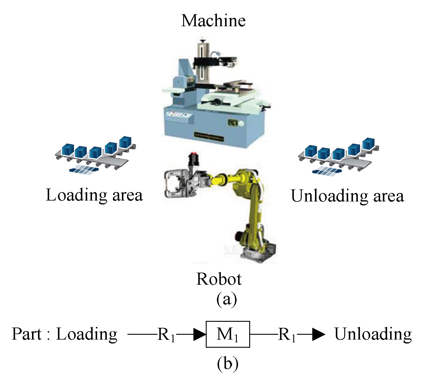
5. Numerical Example

In this section, an example is used to present the application of the proposed approach. Consider an AMS example illustrated in Figure 15a. Its Petri net model is given in [6,7,15,22,45,46]. The system consists of four machines M1–M4 for processing parts; two robots R1 and R2 for loading and unloading parts. Each machine (robot) can process (hold) one part at a time. There are two input buffers I1 and I2 and two output buffers O1 and O2. Two raw part types, A and B, are considered to be processed in the system. Figure 15b shows the operation sequences of the two raw part types. The S³PR net of this AMS example is illustrated in Figure 16. It comprises 19 places and 14 transitions. The places can be defined as the following set partitions: P_A = {p₂, p₃, …, p₁₂}, P_R = {p₁₃, p₁₄, …, p₁₈}, and P⁰ = {p₁, p₁₉}. The S³PR net contains 282 reachable markings.

Suppose that the first configuration of the system involves removing old machine. In this case, an old machine M1 is removed from the system (N_o, M_o). To model the removed machine by using the synthesis procedure of Algorithm 1, we construct a configuration as a rewriting rule $ℛ$= {rr₁} with rr₁ = {L₁, R₁, φ₁, ^•φ₁, φ₁^•}, where L₁ and R₁ are illustrated in Figure 17a and Figure 17b, respectively. In addition, we have ξ₁: N₁ → N_o, φ₁= ({p₂, p₃, p₄, p₅, p₁₃, p₁₆, p₁₇},{t₁, t₂, t₃, t₄, t₅, t₆}), ^•φ₁= ({L₁.t₁},{R₁.t₁}), and φ₁^• = ({L₁.t₆},{R₁.t₆}). The second configuration includes adding new product. If a new product (part C) is assigned to a system, which indicates that a new operation sequence is assigned and the system requires an adjustment to its Petri net model structure. To model the addition of new product by using the synthesis procedure of Algorithm 1, we construct a configuration as a rewriting rule $ℛ$ = {rr₂} with rr₂ = {L₂, R₁, φ₂, ^•φ₂, φ₂^•}, where L₂ and R₂ are illustrated in Figure 18a and Figure 18b, respectively. Moreover, we have ξ₂: N₂ → N₁, φ₂= ({p₁₅, p₁₇, p₂₀, p₂₁, p₂₂, p₂₃},{t₁₅, t₁₆, t₁₇, t₁₈}), ^•φ₂= ({L₂.p₁₅, L₂.p₁₇},{R₂.t₁₅}), and φ₂^• = ({L₂.p₁₅, L₂.p₁₇},{R₂.t₁₈}).

The third system configuration involves rework. In this scenario, a part can be inspected after all operations have been completed. By using the proposed Algorithm 1, the production operations of the reworked part can be exactly and easily modeled by considering rework operations as alternative sequences. Suppose that an inspection machine M5 is added to a system and that part A is processed in M1 and M3. Then, part A is moved to an M5 by Robot 2 to check if there are defects in part A. If part A performs properly, then it will leave the system by Robot 2. Otherwise, if part A has defects, rework is needed, and part A is moved to M3 by Robot 2. To model the rework operation by using the synthesis procedure of Algorithm 1, we construct a configuration as a rewriting rule $ℛ$ = {rr₃} with rr₃ = {L₃, R₃, φ₃, ^•φ₃, φ₃^•}, where L₃ and R₃ are illustrated in Figure 19a and Figure 19b, respectively, ξ₃: N₃ → N₂, φ₃= ({p₆, p₇, p₁₄, p₁₈, p₂₄, p₂₅, p₂₆, p₂₇},{t₆, t₇, t₈, t₁₉, t₂₀, t₂₁, t₂₂}), ^•φ₃= ({L₃.t₆},{R₃.t₆}), and φ₃^• = ({L₃.t₈},{R₃.t₂₁}). The Specifications of S³PR net illustrated in Figure 16 under changeable control specifications are shown in

Table 2. The Specifications of S³PR net illustrated in Figure 16 under configurations.

Parameter	Configuration
	An Initial S3PR Net	Removal of an Old Machine	Addition of a New Product	Rework
No. of monitors	5	3	5	10
No. of arcs	21	12	26	48
Liveness	Live	Live	Live	Live
Boundedness	Bounded	Bounded	Bounded	Bounded
Reversibility	Reversible	Reversible	Reversible	Reversible

. In addition, the required monitors using Algorithm 2 of the system illustrated in Figure 16 under changeable control specifications are shown in

Table 3. Required monitors using Algorithm 2 of the system illustrated in Figure 16 under configurations.

Configuration	i	Siphon	•VSi	VSi•	MRCo (Vsi)
An initial S3PR net	1	S1	t7,t13	t1,t9	5
	2	S2	t4,t5,t13	t1,t11	2
	3	S3	t7,t13	t1,t9	4
	4	S4	t7,t11	t1,t9	3
	5	S5	t4,t13	t2,t11	1
Removal of an old machine	1	S1	t4,t13	t1,t9	1
	2	S2	t7,t11	t4,t9	3
	3	S3	t7,t13	t1,t9	4
Addition of a new product	1	S1	t11,t17	t10,t15	1
	2	S2	t4,t13,t17	t1,t10,t15	2
	3	S3	t4,t13	t1,t9	1
	4	S4	t7,t11,t17	t4,t9,t15	3
	5	S5	t7,t13,t17	t1,t9,t15	4
Rework	1	S1	t7	t6,t19	1
	2	S2	t20	t6	2
	3	S3	t6,t20	t7	1
	4	S4	t7,t11,t17	t4,t9,t15,t19	3
	5	S5	t7,t13,t17	t1,t9,t15,t19	4
	6	S6	t11,t17,t20	t4,t9,t15	4
	7	S7	t13,t17,t20	t1,t9,t15	5
	8	S8	t11,t17	t8,t15	1
	9	S9	t4,t13,t17	t1,t10,t15	2
	10	S10	t4,t13	t1,t9	1

.

The controlled net after adding above changeable control specifications is illustrated in Figure 20. The place and arcs of the controller are illustrated with blue lines.

6. Conclusions

This paper develops a novel two-step solution for quick and accurate reconfiguration of supervisory controllers for deadlock control in RMSs with dynamic changes. In the first step, the net rewriting system is used to design a reconfigurable PN model under dynamic configurations. The obtained model guarantees boundedness behavioral property but may not guarantee the other properties of a Petri net model (i.e., liveness and reversibility). The second step proposes an automatic deadlock prevention policy for reconfigurable Petri net using the siphon control method based on a place invariant to solve the deadlock problem with dynamic structure changes in RMSs and guarantee the liveness and reversibility properties for the system. The proposed method is validated using the GPenSIM tool and compared with existing methods in the literature to highlight its ability of adapting to RMS configuration changes.

The major advantages of the developed approach are as follows: (1) It does not need to compute reachability graphs as illustrated in Algorithm 2, Section 3, and has low-overhead computation as proved in Theorems 10 and 11, Section 4.4. (2) It can automatically and dynamically modify the structure of a Petri net model without affecting its behavioral properties, i.e., liveness, boundedness, and reversibility as illustrated in Algorithm 2, Section 3. (3) It allows rapid reconfigurability and reusability of the controller during reconfiguration as shown in Algorithm 2, Section 3. (4) It can easily handle any dynamical changes in RMSs compared with the studies in Badouel et al. [39], Llorens and Oliver [34], Wu and Zhou [25], and Kaid et al. [7] as shown in Algorithm 2, Section 3. (5) The GPenSIM code is developed for designing, simulation, validation, and performance analysis of deadlock problems with dynamic structure changes in RMSs and the correctness of the proposed approach is proven and compared with the studies in Ezpeleta et al. [43], Li and Zhou [44], and Kaid et al. [6] as shown in Section 4.5. (6) Based on Theorems 10 and 11, the computational complexity of the proposed approach has polynomial time complexity. Therefore, it has low computational complexity and can be applicable to other types of complex systems such as mass customization manufacturing, lean productivity, agile manufacturing, and flexible manufacturing systems. (7) It can consider systems with sequential and complex resource requirements, meaning that a set of system resources can be used and shared to process each component according to sequential processes that depend on the step-by-step discrete execution and multiple processes that depend on the execution at the same time as shown in numerical example.

The limitation of the developed approach is that the obtained models lack an appropriate conversion approach from the PN model into control languages for application. Thus, our future research will examine the developed approach to have an automatic method to examine the applicability of the obtained models for real world manufacturing systems.

References

1. Hu, Y.; Ma, Z.; Li, Z. Design of Supervisors for Active Diagnosis in Discrete Event Systems. IEEE Trans. Autom. Control 2020. [Google Scholar] [CrossRef]
2. Wang, D.; Wang, X.; Li, Z. Nonblocking Supervisory Control of State-Tree Structures with Conditional-Preemption Matrices. IEEE Trans. Ind. Inform. 2019, 16, 3744–3766. [Google Scholar] [CrossRef]
3. Mehrabi, M.G.; Ulsoy, A.G.; Koren, Y. Reconfigurable manufacturing systems: Key to future manufacturing. J. Intell. Manuf. 2000, 11, 403–419. [Google Scholar] [CrossRef]
4. Katz, R. Design principles of reconfigurable machines. Int. J. Adv. Manuf. Technol. 2007, 34, 430–439. [Google Scholar] [CrossRef]
5. Patel, R.; Gojiya, A.; Deb, D. Failure Reconfiguration of Pumps in Two Reservoirs Connected to Overhead Tank. In Innovations in Infrastructure; Springer: Berlin/Heidelberg, Germany, 2019; pp. 81–92. [Google Scholar]
6. Kaid, H.; Al-Ahmari, A.; Li, Z.; Davidrajuh, R. Single controller-based colored Petri nets for deadlock control in automated manufacturing systems. Processes 2020, 8, 21. [Google Scholar] [CrossRef] [Green Version]
7. Kaid, H.; Al-Ahmari, A.; Li, Z.; Davidrajuh, R. Intelligent colored token Petri nets for modeling, control, and validation of dynamic changes in reconfigurable manufacturing systems. Processes 2020, 8, 358. [Google Scholar] [CrossRef] [Green Version]
8. Li, Z.; Zhou, M. Deadlock Resolution in Automated Manufacturing Systems: A Novel Petri Net Approach; Springer Science & Business Media: Berlin/Heidelberg, Germany, 2009. [Google Scholar]
9. Zan, X.; Wu, Z.; Guo, C.; Yu, Z. A Pareto-based genetic algorithm for multi-objective scheduling of automated manufacturing systems. Adv. Mech. Eng. 2020, 12, 1687814019885294. [Google Scholar] [CrossRef]
10. Li, L.; Basile, F.; Li, Z. An approach to improve permissiveness of supervisors for GMECs in time Petri net systems. IEEE Trans. Autom. Control 2019, 65, 237–251. [Google Scholar] [CrossRef]
11. Liu, Y.; Cai, K.; Li, Z. On scalable supervisory control of multi-agent discrete-event systems. Automatica 2019, 108, 108460. [Google Scholar] [CrossRef] [Green Version]
12. Chen, Q.; Yin, L.; Wu, N.; El-Meligy, M.A.; Sharaf, M.A.F.; Li, Z. Diagnosability of vector discrete-event systems using predicates. IEEE Access 2019, 7, 147143–147155. [Google Scholar] [CrossRef]
13. Kaid, H.; Al-Ahmari, A.; Nasr, E.A.; Al-Shayea, A.; Kamrani, A.K.; Noman, M.A.; Mahmoud, H.A. Petri Net Model Based on Neural Network for Deadlock Control and Fault Detection and Treatment in Automated Manufacturing Systems. IEEE Access 2020, 8, 103219–103235. [Google Scholar] [CrossRef]
14. Zhao, M. An integrated control method for designing non-blocking supervisors using Petri nets. Adv. Mech. Eng. 2017, 9, 1687814017700829. [Google Scholar] [CrossRef]
15. Chen, Y.; Li, Z.; Khalgui, M.; Mosbahi, O. Design of a maximally permissive liveness-enforcing Petri net supervisor for flexible manufacturing systems. Autom. Sci. Eng. IEEE Trans. 2011, 8, 374–393. [Google Scholar] [CrossRef]
16. Al-Ahmari, A.; Kaid, H.; Li, Z.; Davidrajuh, R. Strict Minimal Siphon-Based Colored Petri Net Supervisor Synthesis for Automated Manufacturing Systems with Unreliable Resources. IEEE Access 2020. [Google Scholar] [CrossRef]
17. Kaid, H.; Al-Ahmari, A.; El-Tamimi, A.M.; Abouel Nasr, E.; Li, Z. Design and implementation of deadlock control for automated manufacturing systems. South Afr. J. Ind. Eng. 2019, 30, 1–23. [Google Scholar] [CrossRef] [Green Version]
18. Chao, D.Y. Improvement of suboptimal siphon-and FBM-based control model of a well-known S3PR. IEEE Trans. Autom. Sci. Eng. 2011, 8, 404–411. [Google Scholar] [CrossRef]
19. Ghaffari, A.; Rezg, N.; Xie, X. Design of a live and maximally permissive Petri net controller using the theory of regions. IEEE Trans. Robot. Autom. 2003, 19, 137–141. [Google Scholar] [CrossRef]
20. Uzam, M. The use of the Petri net reduction approach for an optimal deadlock prevention policy for flexible manufacturing systems. Int. J. Adv. Manuf. Technol. 2004, 23, 204–219. [Google Scholar] [CrossRef]
21. Sun, D.; Chen, Y.; El-Meligy, M.A.; Sharaf, M.A.F.; Wu, N.; Li, Z. On algebraic identification of critical states for deadlock control in automated manufacturing systems modeled with Petri nets. IEEE Access 2019, 7, 121332–121349. [Google Scholar] [CrossRef]
22. Nasr, E.A.; El-Tamimi, A.M.; Al-Ahmari, A.; Kaid, H. Comparison and Evaluation of Deadlock Prevention Methods for Different Size Automated Manufacturing Systems. Math. Probl. Eng. 2015, 501, 1–19. [Google Scholar] [CrossRef] [Green Version]
23. Lee, S.; Tilbury, D.M. Deadlock-free resource allocation control for a reconfigurable manufacturing system with serial and parallel configuration. IEEE Trans. Syst. ManCybern. Part C (Appl. Rev.) 2007, 37, 1373–1381. [Google Scholar] [CrossRef]
24. Li, J.; Dai, X.; Meng, Z. Automatic reconfiguration of petri net controllers for reconfigurable manufacturing systems with an improved net rewriting system-based approach. IEEE Trans. Autom. Sci. Eng. 2009, 6, 156–167. [Google Scholar] [CrossRef]
25. Wu, N.; Zhou, M. Intelligent token Petri nets for modelling and control of reconfigurable automated manufacturing systems with dynamical changes. Trans. Inst. Meas. Control 2011, 33, 9–29. [Google Scholar]
26. Sampath, R.; Darabi, H.; Buy, U.; Liu, J. Control reconfiguration of discrete event systems with dynamic control specifications. IEEE Trans. Autom. Sci. Eng. 2008, 5, 84–100. [Google Scholar] [CrossRef]
27. Dumitrache, I.; Caramihai, S.; Stanescu, A. Intelligent agent-based control systems in manufacturing. In Proceedings of the 2000 IEEE International Symposium on Intelligent Control. Held jointly with the 8th IEEE Mediterranean Conference on Control and Automation (Cat. No. 00CH37147), Rio Patras, Greece, 19–19 July 2000; pp. 369–374. [Google Scholar]
28. Ohashi, K.; Shin, K.G. Model-based control for reconfigurable manufacturing systems. In Proceedings of the 2001 ICRA. IEEE International Conference on Robotics and Automation (Cat. No. 01CH37164), Seoul, Korea, 21–26 May 2001; pp. 553–558. [Google Scholar]
29. Kalita, D.; Khargonekar, P.P. Formal verification for analysis and design of logic controllers for reconfigurable machining systems. IEEE Trans. Robot. Autom. 2002, 18, 463–474. [Google Scholar] [CrossRef]
30. Almeida, E.E.; Luntz, J.E.; Tilbury, D.M. Event-condition-action systems for reconfigurable logic control. IEEE Trans. Autom. Sci. Eng. 2007, 4, 167–181. [Google Scholar] [CrossRef]
31. Zhang, L.; Rodrigues, B. Modelling reconfigurable manufacturing systems with coloured timed Petri nets. Int. J. Prod. Res. 2009, 47, 4569–4591. [Google Scholar] [CrossRef]
32. Kahloul, L.; Bourekkache, S.; Djouani, K.; Chaoui, A.; Kazar, O. Using high level Petri nets in the modelling, simulation and verification of reconfigurable manufacturing systems. Int. J. Softw. Eng. Knowl. Eng. 2014, 24, 419–443. [Google Scholar] [CrossRef]
33. Yu, Z.; Guo, F.; Ouyang, J.; Zhou, L. Object-oriented Petri nets and π-calculus-based modeling and analysis of reconfigurable manufacturing systems. Adv. Mech. Eng. 2016, 8, 1687814016677698. [Google Scholar] [CrossRef] [Green Version]
34. Llorens, M.; Oliver, J. Structural and dynamic changes in concurrent systems: Reconfigurable Petri nets. IEEE Trans. Comput. 2004, 53, 1147–1158. [Google Scholar] [CrossRef]
35. Li, J.; Dai, X.; Meng, Z. Improved net rewriting systems-based rapid reconfiguration of Petri net logic controllers. In Proceedings of the 31st Annual Conference of IEEE Industrial Electronics Society, Raleigh, NC, USA, 6–10 November 2005. [Google Scholar]
36. da Silva, R.M.; Benítez-Pina, I.F.; Blos, M.F.; Santos Filho, D.J.; Miyagi, P.E. Modeling of reconfigurable distributed manufacturing control systems. IFAC-Pap. 2015, 48, 1284–1289. [Google Scholar] [CrossRef]
37. Berthomieu, B.; Ribet, P.-O.; Vernadat, F. The tool TINA–construction of abstract state spaces for Petri nets and time Petri nets. Int. J. Prod. Res. 2004, 42, 2741–2756. [Google Scholar] [CrossRef]
38. Bonet, P.; Catalina, M.L.; Puigjaner, R. A Petri Net tool for performance modeling. In Proceedings of the 23rd Latin American Conference on Informatics (CLEI 2007), San Jose, Costa Rica, October 2007. [Google Scholar]
39. Badouel, E.; Llorens, M.; Oliver, J. Modeling concurrent systems: Reconfigurable nets. In Proceedings of the PDPTA, Las Vegas, NV, USA, 23–26 June 2003; pp. 1568–1574. [Google Scholar]
40. Yamalidou, K.; Moody, J.; Lemmon, M.; Antsaklis, P. Feedback control of Petri nets based on place invariants. Automatica 1996, 32, 15–28. [Google Scholar] [CrossRef]
41. Moody, J.O.; Antsaklis, P.J. Supervisory Control of Discrete Event Systems Using Petri Nets; Springer Science & Business Media: Berlin/Heidelberg, Germany, 2012; Volume 8. [Google Scholar]
42. Davidrajuh, R. Modeling Discrete-Event Systems with GPenSIM: An Introduction; Springer: Berlin/Heidelberg, Germany, 2018. [Google Scholar]
43. Ezpeleta, J.; Colom, J.M.; Martinez, J. A Petri net based deadlock prevention policy for flexible manufacturing systems. IEEE Trans. Robot. Autom. 1995, 11, 173–184. [Google Scholar] [CrossRef] [Green Version]
44. Li, Z.; Zhou, M. Elementary siphons of Petri nets and their application to deadlock prevention in flexible manufacturing systems. IEEE Trans. Syst. Man Cybern. Part A Syst. Hum. 2004, 34, 38–51. [Google Scholar] [CrossRef]
45. Piroddi, L.; Cordone, R.; Fumagalli, I. Selective siphon control for deadlock prevention in Petri nets. IEEE Trans. Syst. Man Cybern. Part A: Syst. Hum. 2008, 38, 1337–1348. [Google Scholar] [CrossRef]
46. Chen, Y.; Li, Z.; Zhou, M. Behaviorally optimal and structurally simple liveness-enforcing supervisors of flexible manufacturing systems. IEEE Trans. Syst. Man Cybern. Part A Syst. Hum. 2012, 42, 615–629. [Google Scholar] [CrossRef]
Figure 1. (a) Automated manufacturing system (AMS) example and (b) operation sequence.
Applsci 10 05270 g001
Figure 2. A system of (S2P) (simple sequential process) (S3PR) net of the AMS.
Applsci 10 05270 g002
Figure 3. A reconfigured S3PR net by addition of new machine. (a) Left hand side net L. (b) Right hand side net R. (c) A reconfigurable S3PR net (N1, M1o).
Applsci 10 05270 g003
Figure 4. A reconfigured S3PR net by addition of new product. (a) Left hand side net L. (b) Right hand side net R. (c) A reconfigurable S3PR net (N2, M2o).
Applsci 10 05270 g004
Figure 5. A reconfigured S3PR net by rework. (a) Left hand side net L. (b) Right hand side net R. (c) A reconfigurable S3PR net (N3, M3o).
Applsci 10 05270 g005
Figure 6. A reconfigured S3PR net by addition of a new robot. (a) Left hand side net L. (b) Right hand side net R. (c) A reconfigurable S3PR net (N4, M4o).
Applsci 10 05270 g006
Figure 7. Controlled S3PR net by Algorithm 2.
Applsci 10 05270 g007
Figure 8. Controlled reconfigurable S3PR net by addition of new machine.
Applsci 10 05270 g008
Figure 9. Controlled reconfigurable S3PR net by addition of new product.
Applsci 10 05270 g009
Figure 10. Controlled reconfigurable S3PR net by rework.
Applsci 10 05270 g010
Figure 11. Controlled reconfigurable S3PR net by rework.
Applsci 10 05270 g011
Figure 12. Reachable markings of a controlled reconfigurable S3PR net, as illustrated in Figure 8.
Applsci 10 05270 g012
Figure 13. Reachable markings of a controlled reconfigurable S3PR net, as illustrated in Figure 7.
Applsci 10 05270 g013
Figure 14. Comparison of the proposed method with the existing methods.
Applsci 10 05270 g014
Figure 15. (a) An AMS example and (b) production sequence.
Applsci 10 05270 g015
Figure 16. S3PR net (No, Mo) of the AMS illustrated in Figure 13a.
Applsci 10 05270 g016
Figure 17. A reconfigured S3PR net by removing a machine. (a) Left hand side net L. (b) Right hand side net R.
Applsci 10 05270 g017
Figure 18. A reconfigured S3PR net by adding a product. (a) Left hand side net L. (b) Right hand side net R.
Applsci 10 05270 g018
Figure 19. A reconfigured S3PR net by rework. (a) Left hand side net L. (b) Right hand side net R.
Applsci 10 05270 g019
Figure 20. Controlled reconfigurable S3PR net after adding changeable control specifications.
Applsci 10 05270 g020