Estimating Degradation Costs for Non-Cyclic Usage of Lithium-Ion Batteries

Abstract

Estimating the degradation costs of lithium-ion batteries is essential to the designs of many systems because batteries are increasingly used in diverse applications. In this study, cyclic and calendar degradation models of lithium batteries were considered in optimization problems with randomized non-cyclic batteries use. Such models offer realistic results. Electrical, thermal, and degradation models were applied for lithium nickel cobalt manganese oxide (NMC) and lithium iron phosphate (LFP) technologies. Three possible strategies were identified to estimate degradation costs based on cell models. All three strategies were evaluated via simulations and validated by comparing the results with those obtained by other authors. One strategy was discarded because it overestimates costs, while the other two strategies give good results, and are suitable for estimating battery degradation costs in optimization problems that require deterministic models.

1. Introduction

This study aims to determine which cell technology models are most suitable for estimating batteries’ degradation costs to determine the most appropriate model for use in optimization problems. It is common to consider two types of battery degradation: calendar and cyclic. Calendar degradation occurs when a battery is at rest, i.e., when it is neither being charged nor discharged. Cyclic degradation occurs when the battery is being charged or discharged. In lithium-ion batteries, the main reason for calendar degradation is an increase in the solid electrolyte interface layer on the negative (graphite) electrode. In cyclic degradation, the most crucial reason is the accumulation of lithium on the negative electrode [1].

In this work, we reviewed and applied the most suitable models for estimating calendar degradation and for evaluating cyclic degradation.

Battery degradation costs can be an essential economic variable when designing an installation with battery power storage [2]. Several models in the technical literature can estimate batteries’ degradation costs, sometimes including thermal and electrical aspects [3,4,5,6,7]. Depending on the significance of the degradation costs, the best solutions may or may not include extensive use of the batteries. These solutions often include random battery use that differs from standard cyclic usage. It is necessary to estimate degradation costs accurately. While selecting the models studied, the fact that the feedback of values in real-time is not available when mathematical models are used for optimization problems were taken into account [6,7].

There are several papers with literature reviews of degradation models. Pelletier et al. [3] analyzed several models, including those of Wang et al. [8,9,10]; Sarasketa-Zabala et al. [11,12,13,14]; Hoke et al. [15]; Omar et al. [16], and; Han et al. [17]. In other reviews, Thompson [4] studied and identified three main models: NREL, Wang, and MOBICUS; and Lucu et al. [5] reviewed adaptive aging models, which are of interest for on-board systems but not for our objective. The review carried out by Jafari et al. [6] is useful for optimization problems; this review presented deterministic models that are easy to apply, as they provide functions fitted to real data. Finally, a review by Ahmadian et al. [7] is of interest, in which several classifications of mathematical model studies related to battery degradation were presented.

Several degradation models have been applied to optimization problems. Dufo-López et al. [2] applied several battery aging models developed for the optimization of lead-acid batteries, and García Vera et al. [18] also applied various battery life models to the optimization of off-grid systems, considering both lead-acid and lithium-ion batteries. Due to their increasing use, a detailed study of lithium-ion battery life models is necessary in order to be able to apply them to this type of problem.

The degradation of lithium nickel cobalt aluminum oxide (NCA) cells is treated by Hoke et al. [15] with a simplified lifetime model applied to the optimization of electric vehicle charging. The battery life model estimates both energy capacity fading and power fading due to temperature, state of charge profile, and daily depth of discharge (DoD).

In another study of lithium-ion batteries, Schmalstieg et al. [19] fitted functions for capacity and internal resistance based on data obtained from Ecker et al. [20]. They modeled calendar loss and cyclic loss. Capacity fade and resistance growth due to calendar degradation depend on cell voltage (V), absolute surface cell temperature (T), and the actual time of cell life (t). Capacity fade and resistance growth due to cyclic usage depend on average voltage, DoD or depth of cycle for NMC (DoD), and total Ah-throughput from the beginning of cell life (Q). Considering another cell technology, the Zabala model provides cyclic and calendar degradation of an LFP/graphite 26650-type cell of 2.3 Ah and 3.3 V. It is described in four studies by Sarasketa-Zabala et al. First, calendar degradation and cyclic degradation models were introduced [11], then only the calendar model was studied [12]. The cyclic degradation model was adjusted again [13], and finally, the two degradations were revisited [14]. Modeling of total degradation was achieved, including cyclic and calendar types.

Electrochemical models are usually very complex, so they are unsuitable for optimization problems because there are many possible solutions, a high number of evaluations, and therefore excessive calculation times. The models of Astaneh et al. [21,22], Xiong et al. [23], Wijewardana et al. [24], Suresh et al. [25,26], and Ashwin et al. [27,28] are examples. A simplified electrochemical model is provided by Rechkemmer et al. [29]. They proposed a hybridization of the single-particle model and an electrical equivalent model, with better computation time than a single-particle model and more accuracy than an electrical equivalent model. Pelletier et al. [3], to include variations in operating conditions, determined that based on the work of Sarasketa-Zabala et al. [12,13], the heterogeneous use of a cell can be taken into account by considering the conditions of a specific use of the cell at an initial degradation state resulting from the end of its previous use.

Other studies, on the health prognosis of lithium batteries, achieved very satisfactory results predicting batteries’ end of life, such as one carried out by Li et al. [30]. In the present work, however, we have not considered that study, or similar ones, because no studies about the prognostics and health management applicable to our purpose are founded. Previous studies use some parameters adjusted to replicate experimental data, with expressions that depend on full equivalent cycles and on other abstract parameters. It is not clear the relation with cell properties and with usage conditions like DoD, CR; or temperature can be used to parametrize cell charges/discharges and rest time. The revised works are based on experiments performed that considered little cyclic usage and a reduced variety of conditions.

In addition to the availability of degradation models, the cost associated with the reduction of battery life needs to be appropriately assessed. Several authors have applied various methodologies in order to assess this cost.

Han et al. [17] used a ratio of total energy transferred over the complete lifetime of the battery. Song et al. [31] used the derivative of capacity loss over time and applied it at the current point in time of cell life. Wang et al. [10] applied a similar strategy; they used the derivative of capacity loss over time and multiplied it by the time of use.

Two indicators commonly used to measure battery degradation are the capacity fade (CF), which relates to capacity loss, and the power fade (PF), which relates to the increase of internal resistance.

Uddin et al. [32] obtained the degradation cost (Cost_deg) from CF, PF, and battery replacement cost (Cost_bat). CF is a function that depends on several parameters of the equivalent circuit model: cell remaining capacity at a given time (C), capacity at the beginning of life (C_BOL), and the cell capacity factor at the end of life compared to the beginning of life (µ_CF). Furthermore, they defined PF as a function that depends on ohmic resistance of the cell (R₀), charge transfer resistance of the cell (R₁), the ohmic resistance of the cell at the beginning of life (R_0,BOL), charge transfer resistance of the cell at the beginning of life (R_1,BOL), and the cell total resistance factor at the end of life compared to the beginning of life (µ_PF).

$$CF=1-\frac{C\left(t\right)-{\mu }_{CF}{C}_{BOL}}{C_{BOL}-{\mu }_{CF}{C}_{BOL}}=\frac{C_{BOL}-C\left(t\right)}{C_{BOL}-{\mu }_{CF}{C}_{BOL}},$$

(1)

$$PF=\frac{1}{{\mu }_{PF}-1}\left(\frac{R_0\left(t\right)+R_1\left(t\right)}{R_{0,BOL}+R_{1,BOL}}-1\right),$$

(2)

$$Cos{t}_{deg}=\max \left(CF·Cos{t}_{bat},PF·Cos{t}_{bat}\right),$$

(3)

where µ_CF is 0.8, as the capacity degradation at the end of life is 20%. Moreover, µ_PF is 2, as the increase in total resistance at the end of life is 100%.

In Equations (1) and (2), the terms C, R_0,BOL, and R_1,BOL are expressed as C(t), R₀(t), and R₁(t) to reinforce the idea that they change over time, and the other terms are constants.

Other authors applied different methodologies. Weitzel et al. [33] multiplied the Cost_bat by the ratio of magnitude involved in actual use to the same magnitude over the battery lifetime. For the calendar cost, the magnitude used is time, and for cyclic cost, it is Ah-throughput. Liu et al. [34] used battery degradation to achieve better strategies in charging batteries, applying a multi-objective approach in a market with different hourly energy prices. They obtained degradation cost as a fraction of battery replacement cost, proportional to the used Ah-throughput.

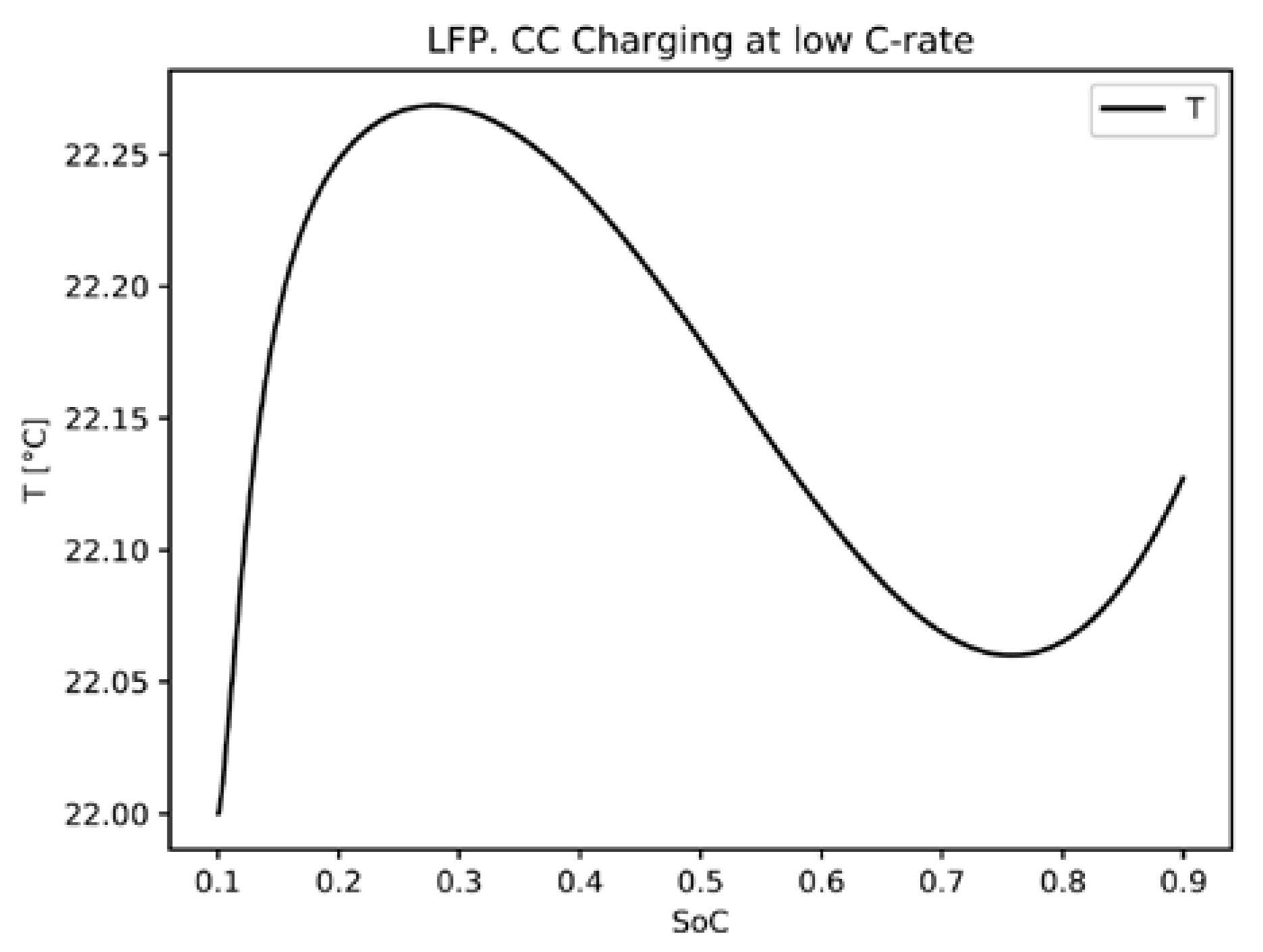
Sometimes calculating degradation costs requires a dynamic simulation of the cell during the charge, discharge, and rest periods. Using a simulation with the current applied and ambient temperature as inputs, the output values of voltage and cell temperature can be obtained. For this purpose, the most commonly used electric model is the Thevenin model. It consists of a voltage source named open circuit voltage (OCV), a serial resistance, and an RC circuit, as seen in Figure 1.

This model is extensively described in the literature; for example, by Hu et al. [35], where the Thevenin model uses hysteresis. A more traditional formulation can be found in Mansour et al. [36], which uses it for the state of charge (SoC) for NMC estimation with adaptive filters, Xiong et al. [37], or Zheng et al. [38].

A similar formulation to that of the above studies was developed by Cordoba-Arenas et al. [39].

Cell temperature depends on cell use and ambient temperature. Models that evaluate the cell temperature take into account that heat generation affects temperature variation. Thus, Jalkanen et al. [40] differentiate reversible heat generation, which is due mainly to entropy change, from irreversible heat generation, which depends on internal resistance and current.

The temperature model applied by Wang et al. [10] uses the thermal heat generated by internal resistance. It models heat transference from/to the battery, ambient atmosphere, and cabin, based on the work of Neubauer et al. [41]. They provide values for the heat transfer coefficient and thermal mass of the battery.

Another study on heat generation is Balasundaram et al. [42], which tests the temperature model on an LFP cell. Song et al. [31] use entropy variation, based on a Forged et al. [43] study that calculates the internal temperature of an LFP/graphite 26,650 cell depending on surface temperature and ambient temperature.

Cordoba-Arenas et al. [39] developed a thermal model with air convection. Wijegardana et al. [24] present a complete thermal model with coefficients for Panasonic 17,500 cells. Furthermore, Uddin et al. [32] report a thermal model applied to 18,650 cells.

Rechkemmer et al. [29] adapted the Schmalstieg model to another cell technology, lithium manganese oxide (LMO); they used a thermal model without entropy variation.

The Thevenin model can also be adapted to reflect degradation. For example, Tang et al. [44] adapted non-degraded cell models to degraded cell models based on data from cell usage.

A thermal model based on reversible and irreversible heat generation and heat transfer from the cell to the ambient atmosphere (useful for our purposes) is available from Wang et al. [10], Balasundaram et al. [42], and Song et al. [31].

2. Materials and Methods

2.1. Electrical and Thermal Models

The electrical model applied in this work is the Thevenin model, as described by Equations (4)–(6), extracted from Cordoba-Arenas et al. [39]. They express the variation over time of the voltage of an RC Thevenin circuit (U), the variation over time of the SoC, and V.

$$\frac{dU\left(t\right)}{dt}=\frac{-1}{R_1{C}_1}U\left(t\right)+\frac{I\left(t\right)}{C_1},$$

(4)

$$\frac{dSoC\left(t\right)}{dt}=\frac{-I\left(t\right)}{C_{BOL}},$$

(5)

$$V\left(t\right)=OCV-R_{0}I\left(t\right)-U\left(t\right),$$

(6)

The Thevenin model for LFP cells is the model proposed by Hu et al. [35], which uses hysteresis. For NMC cells, the formulation can be found in the study by Zheng et al. [38], but also in other studies, for example, that by Mansour et al. [36]. The convention used in this work is that I is positive while discharging.

In the work presented in this paper, the thermal model used is based on reversible and irreversible heat generation and heat transfer from the cell to the ambient atmosphere. The model is derived from Wang et al. [10], Balasundaram et al. [42], and Song et al. [31]. The values used in the model are cell mass (m), the specific heat capacity of the cell (C_p), T, cell-ambient heat transfer coefficient (h), heat transfer surface area of the cell (A), t in seconds, ambient temperature (T_a), OCV, V, and cell current (I). The whole model is expressed in Equation (7).

$$m{C}_p\frac{dT}{dt}=hA\left(T_a-T\right)+I\left(OCV-V\right)+IT\frac{\partial OCV}{\partial T},$$

(7)

where the term I (OCV − V) is the irreversible heat generation, and I T (∂OCV/∂T) is the reversible heat generation due to entropy variation. Heat interchanged between the cell and the atmosphere is modeled by the term h A(T_a−T). The thermal model used is based on Equation (7). The reversible term is always lower than the irreversible term, as stated by Balasundaram et al. [42], and for high CR, the irreversible term is much higher than the reversible one. The reversible heat generation due to entropy variation is ignored.

Simulations were performed applying Equations (8)–(11) with a δ_t of 15 s.

$$T_k=T_{k-1}+\frac{{\delta }_t\left[hA\left(T_a-T_{k-1}\right)+I_{k-1}\left(OC{V}_{k-1}-V_{k-1}\right)\right]}{m{C}_p},$$

(8)

$$So{C}_k=So{C}_{k-1}-\frac{I_{k-1}{\delta }_t}{3600·C_{BOL}},$$

(9)

$$U_k=\exp \left(\frac{-{\delta }_t}{R_{1,k-1}{C}_{1,k-1}}\right)U_{k-1}+\left[1-\exp \left(\frac{-{\delta }_t}{R_{1,k-1}{C}_{1,k-1}}\right)\right]R_{1,k-1}{I}_{k-1},$$

(10)

$$V_k=OC{V}_k-R_{0,k}{I}_k-U_k,$$

(11)

where T, I, V, SoC, and U were discretized. While OCV, R₀, R₁, and surface layer capacitance of cell (C₁) values depend on SoC and T, they were fitted by using several studies on different cell technologies.

2.2. Degradation

In the present study, NMC and LFP cells are used. For NMC cells, the primary reference is Schmalstieg et al. [19], while for LFP cells, the references are Sarasketa-Zabala et al. [11] and Weitzel et al. [32].

Some studies provide two different models, one for CF and another for PF. Nevertheless, several authors, for example, Sarasketa-Zabala et al. [12], Schmalstieg et al. [19], and Uddin et al. [32] conclude that in limiting the cell life, the CF is a better determinant than the PF. Thus, the present study only uses capacity loss and not an increase in internal resistance.

2.2.1. Degradation of NMC Cells

The Schmalstieg et al. [19] study is based on UR18650E commercial NMC cells. It needs a function fitted for OCV, and simulation of SoC and V. It also requires ambient temperature and current profiles.

The calendar capacity loss depends on voltage, cell temperature, and time. Furthermore, cyclic capacity loss depends on an average voltage, DoD, Q, and the total Ah-throughput, but not on charge/discharge current rate (CR).

Equations (12)–(14) formulate, respectively, the remaining cell capacity for NMC technology at a given point in time normalized with C_BOL (C^NMC), calendar capacity loss of NMC technology from the beginning of life normalized with C_BOL ($C_{loss,cal}^{NMC}$), and cyclic capacity loss of NMC technology from the beginning of life normalized with C_BOL ($C_{loss,cyc}^{NMC}$).

$$C^{NMC}=1-C_{loss,cal}^{NMC}-C_{loss,cyc}^{NMC},$$

(12)

$$C_{loss,cal}^{NMC}={\alpha }_{cap}·t^{0.75},$$

(13)

$$C_{loss,cyc}^{NMC}={\beta }_{cap}·\sqrt{Q},$$

(14)

The expressions for α_cap and β_cap depend on V, T, DoD, and quadratic average voltage (V_qa), as shown in Equations (15) and (16).

$${\alpha }_{cap}\left(T,V\right)=\left(7.543V-23.75\right)·{10}^6·e^{\frac{-6976}{T}},$$

(15)

$${\beta }_{cap}\left(V_{qa},DoD\right)=7.348·{10}^{-3}·{(V_{qa}-3.667)}^2+7.6·{10}^{-4}+4.081·{10}^{-3}·DoD,$$

(16)

For V_qa, we apply the value of OCV at the mean SoC of the cycle.

2.2.2. Degradation of LFP Cells

The cell studied by Sarasketa-Zabala et al. [11] and Weitzel et al. [33] is an LFP/graphite 26650-type cell of 2.3 Ah and 3.3 V.

The calendar degradation model is described by Sarasketa-Zabala et al. [11,12,14]. The value of calendar capacity loss of the LFP technology from the beginning of life normalized with C_BOL ($C_{loss,cal}^{LFP}$), a function that depends on SoC, T and t, can be calculated using Equation (17).

$$C_{loss,cal}^{LFP}=S·\exp \left(\alpha ·100·SoC\right)·\exp \left(-\frac{\beta }{T}\right)·t^{\gamma },$$

(17)

where S, α, β, and γ values are defined by [11] (S = 165400, α = 0.01, β = 4148 K, and γ = 0.5). All these parameters were experimentally determined by Sarasketa-Zabala et al. [11].

Sarasketa-Zabala et al. [11] defined a cyclic degradation model that depends on time. Moreover, Weitzel et al. [32] modified this model. The latter study provides an expression for cyclic degradation of capacity while maintaining the same coefficients as those used by Sarasketa-Zabala et al. [11]. The dependency on time is changed to dependency on total Ah-throughput. The cycles used are constant current (CC) cycles.

The value of cyclic capacity loss of LFP cells from the beginning of life normalized with C_BOL ($C_{loss,cyc}^{LFP}$) as a function of DoD, CR, and Q, can be performed using Equations (18)–(20).

$$C_{loss,cyc}^{LFP}=B·K_1·K_2·Q^z,$$

(18)

$$K_1={\alpha }_1+{\alpha }_2·100·DoD+{\alpha }_3·{(100·DoD)}^{0.5}+{\alpha }_4·\ln \left(100·DoD\right),$$

(19)

$$K_2={\beta }_1·C{R}^2+{\beta }_2·CR+{\beta }_3,$$

(20)

where the coefficients B, α₁, α₂, α₃, α₄, β₁, β₂, β_3, and z are extracted from Sarasketa-Zabala et al. [11] and Weitzel et al. [32], this model is valid for CR values above 0.77 and DoD above 3.6%.

2.3. Degradation Cost

Degradation costs at a certain point in time of the cell life are obtained by multiplying the Cost_bat by a value extracted from the degradation model. The methods are obtained from three different visions from the literature and homogenized in the present work. The methods that have been applied, by various authors, for the determination of degradation costs are described below.

Weitzel et al. [33] used the Zabala model, which uses an aging life loss function (ϵ) divided into a calendar aging life loss function (ϵ_cal) and a cyclical aging life loss function (ϵ_cyc) as the factor by which the Cost_bat is multiplied to obtain the Cost_deg. It can be calculated using Equation (21) and is a non-dimensional number.

$$Cos{t}_{deg}=\left({ϵ}_{cal}+{ϵ}_{cyc}\right)Cos{t}_{bat},$$

(21)

Assuming that all cells in a battery are identical, ϵ_cal and ϵ_cyc can be obtained for a single cell, and then used as the ϵ_cal and ϵ_cyc of the entire battery. It is important to note that, in order to obtain a battery Cost_deg, the degradation study of only a single cell is needed.

Weitzel et al. [33] used a replacement cost, uniformly distributed over the whole lifetime of the battery, for the calendar cost, and over the total Ah-throughput used in the cell lifetime for the cyclic cost. A cost proportional to the elapsed time of current use of the battery (Δt) is applied to obtain the calendar cost, and in order to obtain the cyclic cost, a cost proportional to the elapsed Q of the current use of the battery (ΔQ) is applied. The end of battery life is reached when the capacity loss is 20%.

$${ϵ}_{cal}=\frac{\Delta t}{t\left(C_{loss}=20\%\right)},$$

(22)

$${ϵ}_{cyc}=\frac{\Delta Q}{Q\left(C_{loss}=20\%\right)},$$

(23)

where t(C_loss = 20%) and Q(C_loss = 20%) can be obtained from the degradation model.

Uddin et al. [32] applied another strategy, where Cost_deg is related to CF. Applying Equations (1) and (3), as the PF is considered less than the CF, Equation (24) is obtained.

$$Cos{t}_{deg}=CF·Cos{t}_{bat},$$

(24)

Song et al. [31] and Wang et al. [10] used the derivative of capacity over time applied at a certain point in time during the battery life, using Equations (25) and (26).

$$\Delta C_{loss,cal}\left(t\right)=\frac{\partial C_{loss,cal}\left(t\right)}{\partial t}\Delta t,$$

(25)

$$\Delta C_{loss,cyc}\left(t\right)=\frac{\partial C_{loss,cyc}\left(t\right)}{\partial t}\Delta t,$$

(26)

where t is the actual time in the life of a battery.

In this work, we have considered the mathematical models used by other authors, but without using capacity derivatives. Instead of that, the capacity fade increment between two points in time of the cell life before and after a given use of the cell (ΔCF) is used. Then the degradation cost due to the use of a battery can be expressed as:

$$Cos{t}_{deg}=\Delta CF·Cos{t}_{bat}=\frac{C\left(t\right)-C\left(t+\Delta t\right)}{\left(1-{\mu }_{CF}\right)C_{BOL}}·Cos{t}_{bat},$$

(27)

where t is the lifetime previous to the given use of the cell, and t + Δt is the time after that use.

In order to estimate the cost, three different methodologies have been considered (versions 1, 2, and 3). Each of these has different epsilon values. All of them are described below.

2.3.1. Version 1 to Calculate Degradation Costs

Degradation at a particular point in time of cell life is approximated as if the cell were always used at the beginning of its life. The attractiveness of this version is the ease of calculation. As the majority of models predict, degradation speed is higher at the beginning of battery life; thus, an over-estimation for degradation costs is expected.

In version #1, ϵ is considered to be approximately equal to CF. Thus, using Equation (1) we get Equation (28).

$${ϵ}_x=\frac{C_{BOL}-C_x}{C_{BOL}\left(1-{\mu }_{CF}\right)},x\in \left\{cal,cyc\right\},$$

(28)

where C_cal is the capacity reached if only calendar degradation exists, and C_cyc is the capacity reached if only cyclic degradation exists.

Using Equations (9), (10), and (24), the values of the calendar aging life loss function (${ϵ}_{cal}^{NMC}$) and cyclical aging life loss function (${ϵ}_{cyc}^{NMC}$), for NMC cells, can be expressed by Equations (29) and (30).

$${ϵ}_{cal}^{NMC}=\frac{C_{loss,cal}^{NMC}}{1-{\mu }_{CF}}=\frac{{\alpha }_{cap}\left(T,V\right)·t^{0.75}}{1-{\mu }_{CF}},$$

(29)

$${ϵ}_{cyc}^{NMC}=\frac{C_{loss,cyc}^{NMC}}{1-{\mu }_{CF}}=\frac{{\beta }_{cap}\left(V_{qa},DoD\right)·\sqrt{Q}}{1-{\mu }_{CF}},$$

(30)

where V_qa and DoD can be approximated using the maximum SoC over the whole cycle for NMC (SoC_max) and the minimum SoC over the whole cycle for NMC (SoC_min) as in Equations (31) and (32).

$$V_{qa}=OCV\left(\left(So{C}_{max}+So{C}_{min}\right)/2,T\right),$$

(31)

$$DoD=So{C}_{max}-So{C}_{min},$$

(32)

Figure 2a shows ${ϵ}_{cal}^{NMC}$ as a function of the SoC for a range of cell temperatures from 25 to 50 °C, and Figure 2b shows ${ϵ}_{cyc}^{NMC}$ as a function of the DoD, for mean SoC value.

From this, the calculation of cyclic degradation cost due to a single charge or discharge can be realized in one only step. Nevertheless, estimation of calendar degradation cost, if cell parameters change, needs subdivision of time in small increments, considering the parameters as constant over time. This is valid for rest time and for charging or discharging the cell, as well for NMC and LFP cells.

For LFG cells the procedure is similar to that applied to NMC cells, but the supplied capacity loss is expressed as a percentage.

Using Equations (17), (18), and (28), the values of the calendar aging life loss function (${ϵ}_{cal}^{LFP}$) and cyclical aging life loss function (${ϵ}_{cyc}^{LFP}$) can be expressed by Equations (33) and (34):

$${ϵ}_{cal}^{LFP}=\frac{C_{loss,cal}^{LFP}}{100·\left(1-{\mu }_{CF}\right)},$$

(33)

$${ϵ}_{cyc}^{LFP}=\frac{C_{loss,cyc}^{LFP}}{100·\left(1-{\mu }_{CF}\right)},$$

(34)

Figure 3a shows ${ϵ}_{cal}^{LFP}$ as a function of the SoC for a range of cell temperatures from 25 to 50 °C, and Figure 3b shows ${ϵ}_{cyc}^{LFP}$ as a function of the DoD for CR values of 0.77, 0.8, 1, and 2.

2.3.2. Version 2 to Calculate Degradation Costs

This version is based on a uniformly distributed cost over all the life of the battery. It is an approximation used by some authors, for example, Weitzel et al. [33], which estimates that the cost associated with using a battery is the same throughout its life.

In version #2, ϵ can be estimated using Equations (22) and (23). It is necessary to calculate t_cal(C_loss = 20%) and C_cyc(C_loss = 20%), and at end of life CF is equal to 1. This is expressed in Equations (31) and (32):

$$t_{cal}^x\left(C_{loss}=20\%\right)=t_{cal}^x\left(CF=1\right),x\in \left\{NMC,LFP\right\},$$

(35)

$$Q_{cyc}^x\left(C_{loss}=20\%\right)=Q_{cyc}^x\left(CF=1\right),x\in \left\{NMC,LFP\right\},$$

(36)

Using Equations (1) and (13), we can obtain Equation (37), which allows calculation of the time elapsed, throughout the life of the cell, until a certain CF is reached, considering only calendar degradation for NMC cells ($t_{cal}^{NMC}\left(CF\right)$).

$$t_{cal}^{NMC}\left(CF\right)={\left(\frac{C_{loss,cal}^{NMC}}{{\alpha }_{cap}}\right)}^{1/0.75}={\left(\frac{\left(1-{\mu }_{CF}\right)CF}{{\alpha }_{cap}}\right)}^{1/0.75},$$

(37)

Using Equation (14) we can then obtain Equation (38), which allows calculation of the total Ah-throughput used by the cell until a given CF is reached, considering only cyclic degradation for NMC cells ($Q_{cyc}^{NMC}\left(CF\right)$).

$$Q_{cyc}^{NMC}\left(CF\right)={\left(\frac{C_{loss,cyc}^{NMC}}{{\beta }_{cap}}\right)}^2={\left(\frac{\left(1-{\mu }_{CF}\right)CF}{{\beta }_{cap}}\right)}^2,$$

(38)

Using Equations (22), (23), (37), and (38), we obtain Equations (39) and (40), which allow the calculation of ${ϵ}_{cal}^{NMC}$ and ${ϵ}_{cyc}^{NMC}$, with CF equal to 1.

$${ϵ}_{cal}^{NMC}={\left(\frac{{\alpha }_{cap}}{1-{\mu }_{CF}}\right)}^{1/0.75}·\Delta t,$$

(39)

$${ϵ}_{cyc}^{NMC}={\left(\frac{{\beta }_{cap}}{1-{\mu }_{CF}}\right)}^2·\Delta Q,$$

(40)

Figure 4a shows ${ϵ}_{cal}^{NMC}$ as a function of the SoC for a range of cell temperatures from 25 to 50 °C, and Figure 4b shows ${ϵ}_{cyc}^{NMC}$ as a function of the DoD.

Using Equations (1) and (17), we can obtain Equation (41), which allows calculation of the time elapsed throughout the life of the cell until a given CF is reached, considering only calendar degradation for LFP cells ($t_{cal}^{LFP}\left(CF\right)$).

$$t_{cal}^{LFP}\left(CF\right)={\left(\frac{C_{loss,cal}^{LFP}}{f_{cal}^{LFP}\left(SoC,T\right)}\right)}^{1/\gamma }={\left(\frac{100\left(1-{\mu }_{CF}\right)CF}{f_{cal}^{LFP}\left(SoC,T\right)}\right)}^{1/\gamma },$$

(41)

where $f_{cal}^{LFP}$ is evaluated by Equation (42).

$$f_{cal}^{LFP}=A·\exp \left(\alpha ·100·SoC\right)·\exp \left(\frac{-\beta }{T}\right),$$

(42)

From Equation (18) we obtain Equation (43), which allows calculation of the total Ah-throughput used by the cell until a given CF is reached, considering only cyclic degradation for LFP chemistry ($Q_{cyc}^{LFP}\left(CF\right)$).

$$Q_{cyc}^{LFP}\left(CF\right)={\left(\frac{C_{loss,cyc}^{LFP}}{f_{cyc}^{LFP}\left(CR,DoD\right)}\right)}^{1/z}={\left(\frac{100\left(1-{\mu }_{CF}\right)CF}{f_{cyc}^{LFP}\left(CR,DoD\right)}\right)}^{1/z},$$

(43)

where $f_{cyc}^{LFP}$ is evaluated by Equation (44).

$$f_{cyc}^{LFP}=B·K_1·K_2,$$

(44)

Using Equations (22), (23), (41), and (43), we can obtain Equations (45) and (46), which allow calculation of ${ϵ}_{cal}^{LFP}$ and ${ϵ}_{cyc}^{LFP}$, for a $\Delta t$ throughout the life of the cell, where CF is equal to 1.

$${ϵ}_{cal}^{LFP}={\left(\frac{f_{cal}^{LFP}\left(SoC,T\right)}{100\left(1-{\mu }_{CF}\right)}\right)}^{1/\gamma }·\Delta t,$$

(45)

$${ϵ}_{cyc}^{LFP}={\left(\frac{f_{cyc}^{LFP}\left(CR,DoD\right)}{100\left(1-{\mu }_{CF}\right)}\right)}^{1/z}·\Delta Q,$$

(46)

Equations (45) and (46) are the expressions used by Weitzel et al. [32].

Figure 5a shows ${ϵ}_{cal}^{LFP}$ as a function of the SoC for a range of cell temperatures from 25 to 50 °C, and Figure 5b shows ${ϵ}_{cyc}^{LFP}$ as a function of the DoD for CR values of 0.77, 0.8, 1, and 2.

2.3.3. Version 3 to Calculate Degradation Costs

Version #3 aims to obtain the degradation caused by the use of the battery up to a specific moment in its life, using models that allow a high degree of accuracy.

Using Equation (27), we can obtain Equation (47), which allows the evaluation of ϵ.

$$\begin{gathered} {ϵ}_x^y\left(CF\right)=\frac{C_{BOL}-C_{x,act+\Delta }^y}{C_{BOL}\left(1-{\mu }_{CF}\right)}-\frac{C_{BOL}-C_{x,act}^y}{C_{BOL}\left(1-{\mu }_{CF}\right)}=\frac{C_{BOL}-C_{x,act+\Delta }^y}{C_{BOL}\left(1-{\mu }_{CF}\right)}-CF, \\ x\in \left\{cal,cyc\right\},y\in \left\{NMC,LFP\right\} \end{gathered}$$

(47)

where $C_{x,act}^y$ and CF represent, respectively, the current capacity and the capacity fade just before the current use, and $C_{x,act+\Delta }^y$ represents the capacity just after the current use if the only degradation of type x exists.

Using Equations (13), (14), and (47) we can obtain Equations (48) and (49) for NMC cells.

$${ϵ}_{cal}^{NMC}\left(CF\right)=\frac{C_{loss,cal}^{NMC}\left(T,V,t_{cal}^{NMC}\left(CF\right)+\Delta t\right)}{1-{\mu }_{CF}}-CF,$$

(48)

$${ϵ}_{cyc}^{NMC}\left(CF\right)=\frac{C_{loss,cyc}^{NMC}\left(V_{qa},DoD,Q_{cyc}^{NMC}\left(CF\right)+\Delta Q\right)}{1-{\mu }_{CF}}-CF,$$

(49)

Figure 6a shows ${ϵ}_{cal}^{NMC}$ as a function of the SoC for a range of cell temperatures from 25 to 50 °C, and Figure 6b shows ${ϵ}_{cyc}^{NMC}$ as a function of the DoD for CF values of 0.9, 0.5, and 0.1.

Using Equations (17), (18), and (47), we can obtain Equations (50) and (51) for LFP cells.

$${ϵ}_{cal}^{LFP}\left(CF\right)=\frac{C_{loss,cal}^{LFP}\left(SoC,T,t_{cal}^{LFP}\left(CF\right)+\Delta t\right)}{100\left(1-{\mu }_{CF}\right)}-CF,$$

(50)

$${ϵ}_{cyc}^{LFP}\left(CF\right)=\frac{C_{loss,cyc}^{LFP}\left(CR,DoD,Q_{cyc}^{LFP}\left(CF\right)+\Delta Q\right)}{100\left(1-{\mu }_{CF}\right)}-CF,$$

(51)

Figure 7a shows ${ϵ}_{cal}^{LFP}$ as a function of the SoC for a range of cell temperatures from 25 to 50 °C, and Figure 7b shows ${ϵ}_{cyc}^{LFP}$ as a function of the DoD for CR values of 0.77, 0.8, 1, and 2.

2.3.4. Cost Discretization

The costs are evaluated after the electrical and thermal simulations, taking time intervals (δ_t) into account. The methodology applied in this work is based on the idea from Pelletier et al. [3] and Sarasketa-Zabala et al. [12,13], that the heterogeneous use of a cell can be taken into account considering the conditions of a specific cell use, with the cell being at an initial degradation state resulting from the end of the previous cell use.

The ϵ_cyc values are evaluated once for each time interval δ_t with constant current charge or discharge, but not for other intervals. The ϵ_cal is evaluated at every time interval with null current (when the battery is at rest). Finally, all values for all intervals are accumulated to obtain the total ϵ_cal and ϵ_cyc for that simulation.

2.3.5. Comparison of Results

An initial comparison of the results obtained (Figure 2, Figure 3, Figure 4, Figure 5, Figure 6 and Figure 7) shows that ${ϵ}_{cal}^{LFP}$ and ${ϵ}_{cyc}^{LFP}$ are very similar to the data from the original studies of Weitzel et al. [33]. The values of ${ϵ}_{cal}^{NMC}$ and ${ϵ}_{cyc}^{NMC}$ are similar to the data from Schmalstieg et al. [19].

For all cell technologies, version #1 supplies much higher values than versions #2 and #3, while version #2 gives very similar values to #3 when CF is set to 0.5.

The influence of CF in ${ϵ}_{cyc}^{NMC}$, for version #3, is shown in Figure 6b. The ${ϵ}_{cyc}^{NMC}$ values are higher for a lower CF. For CF = 0.9 or 0.5, the results are similar, but for CF = 0.1, values are much higher than for 0.5 and 0.9.

Figure 8 shows the results of several charging and discharging simulations; for SoC = 0.5, the OCV obtained after a charge is approximately 3.7 V for NMC and 3.3 V for LFP, near the respective nominal voltage. The temperature grows while charging and discharging and decreases during rest time, approaching 22 °C, the ambient temperature.

2.4. Data Used in the Simulation

All simulations were performed applying the models described in the previous sections.

For NMC cells, models and data are extracted from literature. For Sanyo UR18650E cells, the cited Schmalstieg et al. [19] degradation model was used. In the present work, OCV is modeled as the fourth-grade polynomial described in Equation (52) fitted with data extracted from Ecker et al. [20]. The cells used by Ecker et al. [20] and Schmalstieg et al. [19] are the same. The Thevenin values used came from Zheng et al. [38], which uses INR18650-20R cells. Thevenin values are considered constants. The nominal voltages of UR18650E and INR18650-20R cells are the same at 3.6 V; thus, it is expected that they are compatible.

$$OC{V}_{NMC}=-3.0208·So{C}^4+7.3282·So{C}^3-5.4919·So{C}^2+2.0406·SoC+3.3339$$

(52)

Table 1. Characteristics of the NMC cell used in the simulations (UR18650E).

Rated Capacity at 20 °C	Nominal Voltage	Maximum Continuous Current		Electrodes
		Charge	Discharge
2050 mAh	3.6 V	1C	3C	Graphite/Li(NiMnCo)O2

shows the main characteristics of the NMC cell used in the simulations.

For LFP cells, the data and models are also extracted from literature. The degradation model used was the Sarasketa-Zabala et al. [11] model fitted for 26,650 cells, and also Weitzel et al. [33], which is based on the Sarasketa-Zabala et al. model [11]. Thevenin values and OCV came from Hu et al. [35], and are fitted for APR18650M1A cells. The models provide functions dependent on SoC and T, and also take into account the hysteresis of LFP cells.

Table 2. Characteristics of the LFP cell used in the simulations (26650).

Rated Capacity	Nominal Voltage	Maximum Continuous Current		Electrodes
		Charge	Discharge
2300 mAh	3.3 V	1C	3C	Graphite/LiFeOP4

shows the main characteristics of the LFP cell used in the simulations.

Parameters of the thermal model were obtained from Cordoba-Arenas et al. [39] and Wijewardana et al. [24].

The same thermal coefficients were used for both cell technologies.

3. Results

3.1. Simulations Performed

The first objective was to reproduce the original results reported in the papers containing the models. This was accomplished for calendar degradation in Figure 2a, Figure 3a, Figure 4a, Figure 5a, Figure 6a, and Figure 7a, using Equations (25), (29), (35), (41), (44), and (46), respectively. For cyclic degradation, the results are in Figure 2b, Figure 3b, Figure 4b, Figure 5b, Figure 6b, and Figure 7b, using Equations (26), (30), (36), (42), (45), and (47), respectively.

In order to test electrical and thermal models, a simulation of combined charge, discharge, and rest time was carried out using Equations (48)–(51). With the current profile and ambient temperature as inputs, the outputs were cell voltage and cell temperature. The simulation involved consecutive 30 min periods of rest, charge, rest, discharge, rest, charge, and rest, with charging and discharging at CC, I = 1.5 A, δ_t = 15 s., and T_a = 22 °C. Figure 8 shows the results of the simulation.

Further, the charging of an LFP cell from 0.1 to 0.9 of the SoC was simulated to verify the temperature model at low CR with T_a = 22 °C, and CR = 0.1 C. Figure 9 shows the temperature variation with respect to SoC.

In order to evaluate individual differences between versions #1, #2, and #3, the root mean square error (RMSE) was applied using version #3 as a reference. Version #3 is used as a reference in order to compare values due to the presumption that version #3 provides results close to real values. Three values of CF were taken into account with version #3: 0.9, 0.5, and 0.1. RMSE was calculated for several values of SoC from 0.0 to 1.0 for calendar degradation and for several values of DoD from 0.0 to 1.0 for cyclic degradation. Parameters used in the RMSE for calendar degradation are shown in

Table 3. Parameters used in root mean square error (RMSE) calculation for calendar degradation.

cal	Δt (h)	Ta (°C)
NMC, LFP	1	25

and

Table 4. Parameters used in RMSE calculation for cyclic degradation.

cyc	ΔQ (Ah)	Vqa (V)	CR
NMC	1	OCV at 0.5 SoC	-
LFP	1	-	1C

for cyclic degradation.

Table 5. Computational time in seconds for 100 cycles of rest, discharge, rest, and charge obtained for the three versions.

Technology	V1	V2	V3
NMC	3.86	3.87	3.95
LFP	14.2	14.3	14.4

and

Table 6. RMSE values of ϵ^NMC, versions #1 and #2. Version #3 as a reference.

	Function	CF = 0.9	CF = 0.5	CF = 0.1
${ϵ}_{cal}^{NMC}$	RMSE(V3,V1)	1.46 × 10−4	1.45 × 10−4	1.39 × 10−4
${ϵ}_{cal}^{NMC}$	RMSE(V3,V2)	1.92 × 10−6	4.72 × 10−7	5.30 × 10−6
${ϵ}_{cyc}^{NMC}$	RMSE(V3,V1)	1.52 × 10−2	1.51 × 10−2	1.40 × 10−2
${ϵ}_{cyc}^{NMC}$	RMSE(V3,V2)	1.31 × 10−4	1.35 × 10−7	1.17 × 10−7

show the resultant RMSE values.

The primary applicability of this study is in optimization problems where the computational time is significant. All calculations in this study were performed on an i5-3340M CPU machine with 4 cores at 2.70 GHz. In order to evaluate computational time for calculation, a single cell charge was simulated. Simulations used to measure the execution time consist of 100 cycles of half an hour rest time, then discharge from 0.9 SoC to 0.2 SoC at 1 CR, then another rest time and then a charge from 0.2 SoC to 0.9 SoC at 1 CR. Table 5 shows, in detail, the computational times for the simulations.

3.2. Interpretation of Simulation Results

As mentioned previously, the results for ${ϵ}_{cal}^{LFP}$ and ${ϵ}_{cyc}^{LFP}$ in Figure 2, Figure 3, Figure 4, Figure 5, Figure 6 and Figure 7 are very similar to the data of Weitzel et al. [33], and the same is true for version #2. Furthermore, the values of ${ϵ}_{cal}^{NMC}$ and ${ϵ}_{cyc}^{NMC}$ agree with the results of Schmalstieg et al. [19].

From Figure 2, Figure 3, Figure 4, Figure 5, Figure 6 and Figure 7, it is clear that in all cases, model version #1 supplies higher values than versions #2 and #3 by several orders of magnitude. Thus, using version #1 as a simplified approximation to degradation cost results in over-estimated values. Moreover, version #2 gives very similar values to #3 with CF = 0.5.

In one case only, ${ϵ}_{cyc}^{NMC}$ in Figure 6b, a visual comparison between the results of version #3 with several CF values shows the influence of actual capacity fade on degradation costs. It clearly shows that lower CF values result in higher degradation costs for the use of a cell. Cell degradation is higher at the beginning of life than at any other time during the cell life.

Version #2 can be considered as an average value taking into consideration the whole cell life. Version #3 with CF = 0.5 is closer to this average value than version #3 with CF = 0.9 or with CF = 0.1.

The results from several charge and discharge cycles shown in Figure 8 are compatible with the cell characteristics. For example, for SoC = 0.5, the OCV value is 3.7 V for the NMC cell. Moreover, the nominal voltage is 3.3 V for the LFP cell. The temperature during rest periods goes to ambient temperature, while it increases during charging and discharging, to a more or less stable value.

A more detailed comparison between the versions can be carried out by looking at the RMSE. The RMSE is shown in Table 6 for NMC, and in

Table 7. RMSE values of ϵ^LFP, versions #1 and #2. Version #3 as a reference.

	Function	CF = 0.9	CF = 0.5	CF = 0.1
${ϵ}_{cal}^{LFP}$	RMSE(V3,V1)	2.74 × 10−3	2.73 × 10−3	2.70 × 10−3
${ϵ}_{cal}^{LFP}$	RMSE(V3,V2)	3.87 × 10−6	1.12 × 10−10	3.48 × 10−5
${ϵ}_{cyc}^{LFP}$	RMSE(V3,V1)	2.41 × 10−4	2.33 × 10−4	2.06 × 10−4
${ϵ}_{cyc}^{LFP}$	RMSE(V3,V2)	1.20 × 10−5	3.62 × 10−6	2.33 × 10−5

for LFP. After reviewing the data in these tables, the following can be stated:

• The estimated degradations using versions #2 and #3 are very similar. All the values of RMSE (#2, #3) are very low, with the only exception of ${ϵ}_{cyc}^{NMC}$ with CF = 1.
• Using version #1, the estimated degradations present the highest values, and applying versions #2 and #3, in all cases, the RMSE is lower than using versions #1 and #3.
• The lowest RMSE between versions #2 and #3 is reached when CF = 0.5 in almost every case, and when it is not, the difference is not relevant. This result is congruent since version #2 is based on constant degradation over all the battery life, degradation estimated by version #3 is higher at the beginning of life, and the degradation grows at a rate that decreases with usage.

Figure 9 shows that discharging at lower CR, cell temperature first increases, then becomes lower before growing again. This effect is also described by Balasundaram et al. [42].

The time consumed by calculations is listed in Table 5. There are no significant differences between versions #1, #2, and #3. In all three cases, the computational time is similar. However, the computational time for NMC is lower than that for LFP. This is due to the complexity of functions fitted for OCV and Thevenin parameters; for the NMC cell, they are quite simple, but for LFP, they are very complex, involving not only a dependency on SoC but also hysteresis and T.

Version #3 is more accurate than versions #1 and #2, and its computational time is only slightly higher than that for the other versions. Thus version #3 is an excellent option to estimate degradation costs.

Other simulations were performed in order to study the performance for a long time. Simulations consist of 100 cycles of rest, discharge, rest, and charge, with the computational time shown in Table 5. After each period of constant current, we calculate the epsilon values, then all of them are used to calculate the RMSE between the reached results (

Table 8. RMSE values of ${ϵ}_{cal}+{ϵ}_{cyc}$, versions #1 and #2 obtained after 100 cycles. Version #3 as a reference.

	Function	CF = 0.9	CF = 0.5	CF = 0.1
NMC	RMSE(V3,V1)	1.78 × 10−2	1.64 × 10−2	1.49 × 10−2
NMC	RMSE(V3,V2)	2.13 × 10−4	4.16 × 10−5	5.38 × 10−4
LFP	RMSE(V3,V1)	1.59 × 10−2	1.59 × 10−2	1.59 × 10−2
LFP	RMSE(V3,V2)	9.53 × 10−6	3.07 × 10−6	1.99 × 10−5

). Comparing Table 6, Table 7 and Table 8, it is clear that the RMSE values are higher in long time periods. In Table 8, versions #2 and #3 provide similar results, and version #1 has a clearly different behavior from the other two versions.

4. Discussion

The present study shows a method to evaluate degradation costs of cells used in irregular non-cyclic charges, discharges, and rest times at periods of constant current. The scale of application is ideal for the optimization of randomized strategies to charge and discharge batteries in the time scale of a day.

Previous models were reviewed for calculating the degradation costs of battery cells. They are based on degradation models. Some congruent deterministic models were found in the literature for two cell technologies, NMC and LFP, combining thermal, electric, and degradation models for compatible cells. They consist of a combination of models and parameters selected to provide a complete solution.

The models were used in simulations, and the results were compared with similar results published by other researchers.

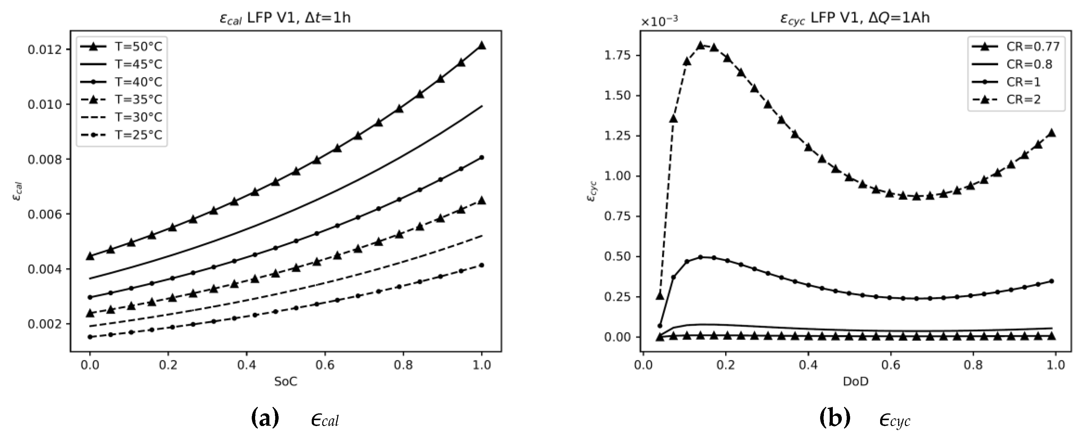
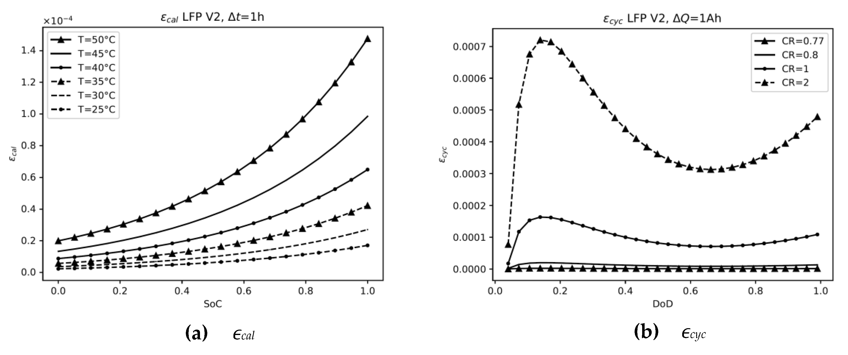
Three strategies for degradation cost estimation were selected, homogenized and evaluated, and it was found that one of them, version #1, based on calculating degradation as if the cell were at the beginning of life, can be discarded due to over-estimation of the costs. Version #2 is based on uniformly distributed degradation throughout the cell life and results in excellent cost estimation. Version #3 uses actual capacity fade as an estimate of the actual age of the cell, and the cost is calculated using degradation models at that CF. The three versions have a similar computational cost. Versions #2 and #3 can estimate more accurate values because they depend on cell CF, providing both similar results. However, version #1 provides results that differ from the other two.

It can be concluded that versions #2 and #3 are good candidates for estimating battery degradation costs in problems where deterministic models are needed, as in the case of optimization problems, since complete charge/discharge cycles are not applied to the batteries.

References

1. Redondo-Iglesias, E.; Venet, P.; Pelissier, S. Modelling lithium-ion battery ageing in electric vehicle applications—Calendar and cycling ageing combination effects. Batteries 2020, 6, 14. [Google Scholar] [CrossRef] [Green Version]
2. Dufo-López, R.; Lujano-Rojas, J.M.; Bernal-Agustín, J.L. Comparison of different lead-acid battery lifetime prediction models for use in simulation of stand-alone photovoltaic systems. Appl. Energy 2014, 115, 242–253. [Google Scholar] [CrossRef]
3. Pelletier, S.; Jabali, O.; Laporte, G.; Veneroni, M. Battery degradation and behaviour for electric vehicles: Review and numerical analyses of several models. Transp. Res. Part B Methodol. 2017, 103, 158–187. [Google Scholar] [CrossRef]
4. Thompson, A.W. Economic implications of lithium ion battery degradation for Vehicle-to-Grid (V2X) services. J. Power Sources 2018, 396, 691–709. [Google Scholar] [CrossRef]
5. Lucu, M.; Martinez-Laserna, E.; Gandiaga, I.; Camblong, H. A critical review on self-adaptive Li-ion battery ageing models. J. Power Sources 2018, 401, 85–101. [Google Scholar] [CrossRef]
6. Jafari, M.; Khan, K.; Gauchia, L. Deterministic models of Li-ion battery aging: It is a matter of scale. J. Energy Storage 2018, 20, 67–77. [Google Scholar] [CrossRef]
7. Ahmadian, A.; Sedghi, M.; Elkamel, A.; Fowler, M.; Aliakbar Golkar, M. Plug-in electric vehicle batteries degradation modeling for smart grid studies: Review, assessment and conceptual framework. Renew. Sustain. Energy Rev. 2018, 81, 2609–2624. [Google Scholar] [CrossRef]
8. Wang, J.; Liu, P.; Hicks-Garner, J.; Sherman, E.; Soukiazian, S.; Verbrugge, M.; Tataria, H.; Musser, J.; Finamore, P. Cycle-life model for graphite-LiFePO4 cells. J. Power Sources 2011, 196, 3942–3948. [Google Scholar] [CrossRef]
9. Wang, J.; Purewal, J.; Liu, P.; Hicks-Garner, J.; Soukazian, S.; Sherman, E.; Sorenson, A.; Vu, L.; Tataria, H.; Verbrugge, M.W. Degradation of lithium ion batteries employing graphite negatives and nickel–cobalt–manganese oxide + spinel manganese oxide positives: Part 1, aging mechanisms and life estimation. J. Power Sources 2014, 269, 937–948. [Google Scholar] [CrossRef]
10. Wang, D.; Coignard, J.; Zeng, T.; Zhang, C.; Saxena, S. Quantifying electric vehicle battery degradation from driving vs. vehicle-to-grid services. J. Power Sources 2016, 332, 193–203. [Google Scholar] [CrossRef] [Green Version]
11. Sarasketa-Zabala, E.; Laresgoiti, I.; Alava, I.; Rivas, M.; Villarreal, I.; Blanco, F. Validation of the methodology for lithium-ion batteries lifetime prognosis. In Proceedings of the 2013 World Electric Vehicle Symposium and Exhibition (EVS27), Barcelona, Spain, 17–20 November 2013; pp. 1–12. [Google Scholar]
12. Sarasketa-Zabala, E.; Gandiaga, I.; Rodriguez-Martinez, L.M.; Villarreal, I. Calendar ageing analysis of a LiFePO4/graphite cell with dynamic model validations: Towards realistic lifetime predictions. J. Power Sources 2014, 272, 45–57. [Google Scholar] [CrossRef]
13. Sarasketa-Zabala, E.; Gandiaga, I.; Martinez-Laserna, E.; Rodriguez-Martinez, L.M.; Villarreal, I. Cycle ageing analysis of a LiFePO4/graphite cell with dynamic model validations: Towards realistic lifetime predictions. J. Power Sources 2015, 275, 573–587. [Google Scholar] [CrossRef]
14. Sarasketa-Zabala, E.; Martinez-Laserna, E.; Berecibar, M.; Gandiaga, I.; Rodriguez-Martinez, L.M.; Villarreal, I. Realistic lifetime prediction approach for Li-ion batteries. Appl. Energy 2016, 162, 839–852. [Google Scholar] [CrossRef]
15. Hoke, A.; Brissette, A.; Maksimović, D.; Pratt, A.; Smith, K. Electric vehicle charge optimization including effects of lithium-ion battery degradation. In Proceedings of the 2011 IEEE Vehicle Power and Propulsion Conference, Chicago, IL, USA, 6–9 September 2011; pp. 1–8. [Google Scholar]
16. Omar, N.; Monem, M.A.; Firouz, Y.; Salminen, J.; Smekens, J.; Hegazy, O.; Gaulous, H.; Mulder, G.; Van den Bossche, P.; Coosemans, T.; et al. Lithium iron phosphate based battery—Assessment of the aging parameters and development of cycle life model. Appl. Energy 2014, 113, 1575–1585. [Google Scholar] [CrossRef]
17. Han, S.; Han, S.; Aki, H. A practical battery wear model for electric vehicle charging applications. Appl. Energy 2014, 113, 1100–1108. [Google Scholar] [CrossRef]
18. García-vera, Y.E.; Dufo-lópez, R.; Bernal-agustín, J.L. Optimization of Isolated Hybrid Microgrids with Renewable Energy Based on Different Battery Models and Technologies. Energies 2020, 13, 581. [Google Scholar] [CrossRef] [Green Version]
19. Schmalstieg, J.; Käbitz, S.; Ecker, M.; Sauer, D.U. A holistic aging model for Li(NiMnCo)O2 based 18650 lithium-ion batteries. J. Power Sources 2014, 257, 325–334. [Google Scholar] [CrossRef]
20. Ecker, M.; Nieto, N.; Käbitz, S.; Schmalstieg, J.; Blanke, H.; Warnecke, A.; Sauer, D.U. Calendar and cycle life study of Li(NiMnCo)O2-based 18650 lithium-ion batteries. J. Power Sources 2014, 248, 839–851. [Google Scholar] [CrossRef]
21. Astaneh, M.; Dufo-López, R.; Roshandel, R.; Golzar, F.; Bernal-Agustín, J.L. A computationally efficient Li-ion electrochemical battery model for long-term analysis of stand-alone renewable energy systems. J. Energy Storage 2018, 17, 93–101. [Google Scholar] [CrossRef]
22. Astaneh, M.; Dufo-López, R.; Roshandel, R.; Bernal-Agustin, J.L. A novel lifetime prediction method for lithium-ion batteries in the case of stand-alone renewable energy systems. Int. J. Electr. Power Energy Syst. 2018, 103, 115–126. [Google Scholar] [CrossRef]
23. Xiong, R.; Li, L.; Li, Z.; Yu, Q.; Mu, H. An electrochemical model based degradation state identification method of Lithium-ion battery for all-climate electric vehicles application. Appl. Energy 2018, 219, 264–275. [Google Scholar] [CrossRef]
24. Wijewardana, S.; Vepa, R.; Shaheed, M.H. Dynamic battery cell model and state of charge estimation. J. Power Sources 2016, 308, 109–120. [Google Scholar] [CrossRef]
25. Suresh, R.; Rengaswamy, R. Modeling and control of battery systems. Part I: Revisiting Butler–Volmer equations to model non-linear coupling of various capacity fade mechanisms. Comput. Chem. Eng. 2018, 119, 336–351. [Google Scholar] [CrossRef]
26. Suresh, R.; Rengaswamy, R. Modeling and control of battery systems. Part II: A model predictive controller for optimal charging. Comput. Chem. Eng. 2018, 119, 326–335. [Google Scholar] [CrossRef]
27. Ashwin, T.R.; Chung, Y.M.; Wang, J. Capacity fade modelling of lithium-ion battery under cyclic loading conditions. J. Power Sources 2016, 328, 586–598. [Google Scholar] [CrossRef] [Green Version]
28. Ashwin, T.R.; McGordon, A.; Widanage, W.D.; Jennings, P.A. Modified electrochemical parameter estimation of NCR18650BD battery using implicit finite volume method. J. Power Sources 2017, 341, 387–395. [Google Scholar] [CrossRef]
29. Rechkemmer, S.K.; Zang, X.; Zhang, W.; Sawodny, O. Empirical Li-ion aging model derived from single particle model. J. Energy Storage 2019, 21, 773–786. [Google Scholar] [CrossRef]
30. Li, X.; Wang, Z.; Yan, J. Prognostic health condition for lithium battery using the partial incremental capacity and Gaussian process regression. J. Power Sources 2019, 421, 56–67. [Google Scholar] [CrossRef]
31. Song, Z.; Li, J.; Han, X.; Xu, L.; Lu, L.; Ouyang, M.; Hofmann, H. Multi-objective optimization of a semi-active battery/supercapacitor energy storage system for electric vehicles. Appl. Energy 2014, 135, 212–224. [Google Scholar] [CrossRef]
32. Uddin, K.; Jackson, T.; Widanage, W.D.; Chouchelamane, G.; Jennings, P.A.; Marco, J. On the possibility of extending the lifetime of lithium-ion batteries through optimal V2G facilitated by an integrated vehicle and smart-grid system. Energy 2017, 133, 710–722. [Google Scholar] [CrossRef]
33. Weitzel, T.; Schneider, M.; Glock, C.H.; Löber, F.; Rinderknecht, S. Operating a storage-augmented hybrid microgrid considering battery aging costs. J. Clean. Prod. 2018, 188, 638–654. [Google Scholar] [CrossRef]
34. Liu, K.; Hu, X.; Yang, Z.; Xie, Y.; Feng, S. Lithium-ion battery charging management considering economic costs of electrical energy loss and battery degradation. Energy Convers. Manag. 2019, 195, 167–179. [Google Scholar] [CrossRef]
35. Hu, X.; Li, S.; Peng, H.; Sun, F. Robustness analysis of State-of-Charge estimation methods for two types of Li-ion batteries. J. Power Sources 2012, 217, 209–219. [Google Scholar] [CrossRef]
36. Mansour, I.; Frisk, E.; Jemni, A.; Krysander, M.; Liouane, N. State of Charge Estimation Accuracy in Charge Sustainable Mode of Hybrid Electric Vehicles. IFAC-PapersOnLine 2017, 50, 2158–2163. [Google Scholar] [CrossRef]
37. Xiong, R.; He, H.; Sun, F.; Zhao, K. Evaluation on State of Charge Estimation of Batteries with Adaptive Extended Kalman Filter by Experiment Approach. IEEE Trans. Veh. Technol. 2013, 62, 108–117. [Google Scholar] [CrossRef]
38. Zheng, F.; Xing, Y.; Jiang, J.; Sun, B.; Kim, J.; Pecht, M. Influence of different open circuit voltage tests on state of charge online estimation for lithium-ion batteries. Appl. Energy 2016, 183, 513–525. [Google Scholar] [CrossRef]
39. Cordoba-Arenas, A.; Onori, S.; Rizzoni, G. A control-oriented lithium-ion battery pack model for plug-in hybrid electric vehicle cycle-life studies and system design with consideration of health management. J. Power Sources 2015, 279, 791–808. [Google Scholar] [CrossRef] [Green Version]
40. Jalkanen, K.; Aho, T.; Vuorilehto, K. Entropy change effects on the thermal behavior of a {LiFePO}4/graphite lithium-ion cell at different states of charge. J. Power Sources 2013, 243, 354–360. [Google Scholar] [CrossRef]
41. Neubauer, J.; Wood, E. Thru-life impacts of driver aggression, climate, cabin thermal management, and battery thermal management on battery electric vehicle utility. J. Power Sources 2014, 259, 262–275. [Google Scholar] [CrossRef]
42. Balasundaram, M.; Ramar, V.; Yap, C.; Li, L.; Tay, A.A.O. Palani Balaya Heat loss distribution: {Impedance} and thermal loss analyses in {LiFePO}4/graphite 18650 electrochemical cell. J. Power Sources 2016, 328, 413–421. [Google Scholar] [CrossRef]
43. Forgez, C.; Vinh Do, D.; Friedrich, G.; Morcrette, M.; Delacourt, C. Thermal modeling of a cylindrical {LiFePO}4/graphite lithium-ion battery. J. Power Sources 2010, 195, 2961–2968. [Google Scholar] [CrossRef]
44. Tang, X.; Wang, Y.; Zou, C.; Yao, K.; Xia, Y.; Gao, F. A novel framework for Lithium-ion battery modeling considering uncertainties of temperature and aging. Energy Convers. Manag. 2019, 180, 162–170. [Google Scholar] [CrossRef]
Figure 1. Thevenin cell model.
Applsci 10 05330 g001
Figure 2. ϵcal and ϵcyc for nickel cobalt manganese oxide (NMC) cells. Version 1.
Applsci 10 05330 g002
Figure 3. ϵcal and ϵcyc for lithium iron phosphate (LFP) cells. Version 1.
Applsci 10 05330 g003
Figure 4. ϵcal and ϵcyc for NMC cells. Version 2.
Applsci 10 05330 g004
Figure 5. ϵcal and ϵcyc for LFP cells. Version 2.
Applsci 10 05330 g005
Figure 6. ϵcal and ϵcyc for NMC cells. Version 3.
Applsci 10 05330 g006
Figure 7. ϵcal and ϵcyc for LFP cells. Version 3.
Applsci 10 05330 g007
Figure 8. Voltage and temperature values. Simulation for NMC and LFP cells for 30 min periods of rest, charge, rest, discharge, rest, charge, and rest. Charging and discharging at CC, I 1.5 A, δt 15 s., and Ta 22 °C.
Applsci 10 05330 g008
Figure 9. LFP cell temperature while charging at low CR.
Applsci 10 05330 g009