Robust Parking Block Segmentation from a Surveillance Camera Perspective

Abstract

Parking block regions host dangerous behaviors that can be detected from a surveillance camera perspective. However, these regions are often occluded, subject to ground bumpiness or steep slopes, and thus they are hard to segment. Firstly, the paper proposes a pyramidal solution that takes advantage of satellite views of the same scene, based on a deep Convolutional Neural Network (CNN). Training a CNN from the surveillance camera perspective is rather impossible due to the combinatory explosion generated by multiple point-of-views. However, CNNs showed great promise on previous works over satellite images. Secondly, even though there are many datasets for occupancy detection in parking lots, none of them were designed to tackle the parking block segmentation problem directly. Given the lack of a suitable dataset, we also propose APKLOT, a dataset of roughly 7000 polygons for segmenting parking blocks from the satellite perspective and from the camera perspective. Moreover, our method achieves more than 50% intersection over union (IoU) in all the testing sets, that is, at both the satellite view and the camera view.

1. Introduction

Parking lots are dynamic environments that brew mishaps of many sorts. A crime investigation report of the Bureau of Justice Statistics of the United States in parking garage facilities states that 9% of crimes in 2010 occurred in parking places [1]. Algorithms for simulating and controlling parking lot behavior, for example, vacant space detection, rely heavily on having parking spot and parking block areas previously marked by a human [2].

In this work, we propose to segment parking blocks in a surveillance camera image. The previously mentioned insecurity problem can then be ameliorated by a second generative algorithm (out of the scope of this work) that take benefit from the priors our proposal produces. This approach was first used for traffic scene analysis in Reference [3], by using dynamic belief (Bayesian) networks. In the same vein, Reference [4] proposes to use prior probabilities of parking block areas of these spaces to guide robot navigation.

Seo [4] also provides a definition for parking blocks in terms of parking spots. We extended this definition to include also partially occluded parking spots and of arbitrary shapes onto splines and containing parking spots of different sizes or neighborhood arrangements.

In brief, segmenting parking blocks means to be able to identify areas in the ground plane that belong to a series of parking blocks, automatically and with high resiliency over the particular surveillance camera view conditions. There are some challenges derived by the problem formulation by itself.

Firstly, an obvious challenge is the different angles and zooms a camera could have. The combinations of the three components of the projection angle and any reasonable zoom level set by the surveillance operator generates an exponentially growing set of possible projection planes. Even though we can still apply an affine transformation to normalize into a simpler domain [5], each pose yields a slightly different set of unrelated features. Considering these changes in the point of view, the most common features can become more or less visible.

Secondly, in the worst case scenario, each scene is particularly packed with a series of occlusions and shadows depending on the particular camera position. This phenomenon introduces a Bayesian noise that is impossible to overcome without lots of data samples.

Third, we also have a broader range of noise sources from the camera perspective in detecting parking spots. [6] categorize them into 3 main sources:

• Typical Attributes. Similar painted lines, other vehicles, kerbstones, non-plain floor, etc.
• Road Conditions. Partially damaged parking lines, paving, etc.
• Surrounding Conditions. Weather, illumination, light source angle, etc.

We can add to this list the presence of occlusions caused by temporal entities like vehicles and pedestrians. Also (but rarer), is the usage of cameras with different settings like color resolution, in the same parking lot.

For these three aforementioned reasons, solving our problem by a mere (self-)supervised algorithm would require an exponential number of samples, and thus is virtually impossible.

In the past 25 years, approaches to solving this problem obviated the use of satellite perspective images available for the same surveillance camera scene. With the advent of modern public Geographic Information Systems (GIS) repositories, high resolution satellite perspective images of outdoor city components became ubiquitous. These satellite perspective images frequently include parking lots, and in some cases, they are even segmented by community members. The satellite perspective allows the following advantages:

• Parking lots are viewed from the space.
• Texture appearance prevails over other features.
• The view is orthogonal.
• Instances can be rotated and form a manifold with the sole condition they do not overlap.
• Variable angle of parking spots relative to the road, no more than 180 degrees.
• Satellite images rarely have shadows and we could remove them by using histogram normalization.

Furthermore, Reference [4] demonstrated that canonical parking spots are easier to detect in those images. Also, Reference [7] provides a good summary of features in the satellite realm.

To take advantage of these previous findings, we propose to segment the parking blocks of the surveillance camera image by:

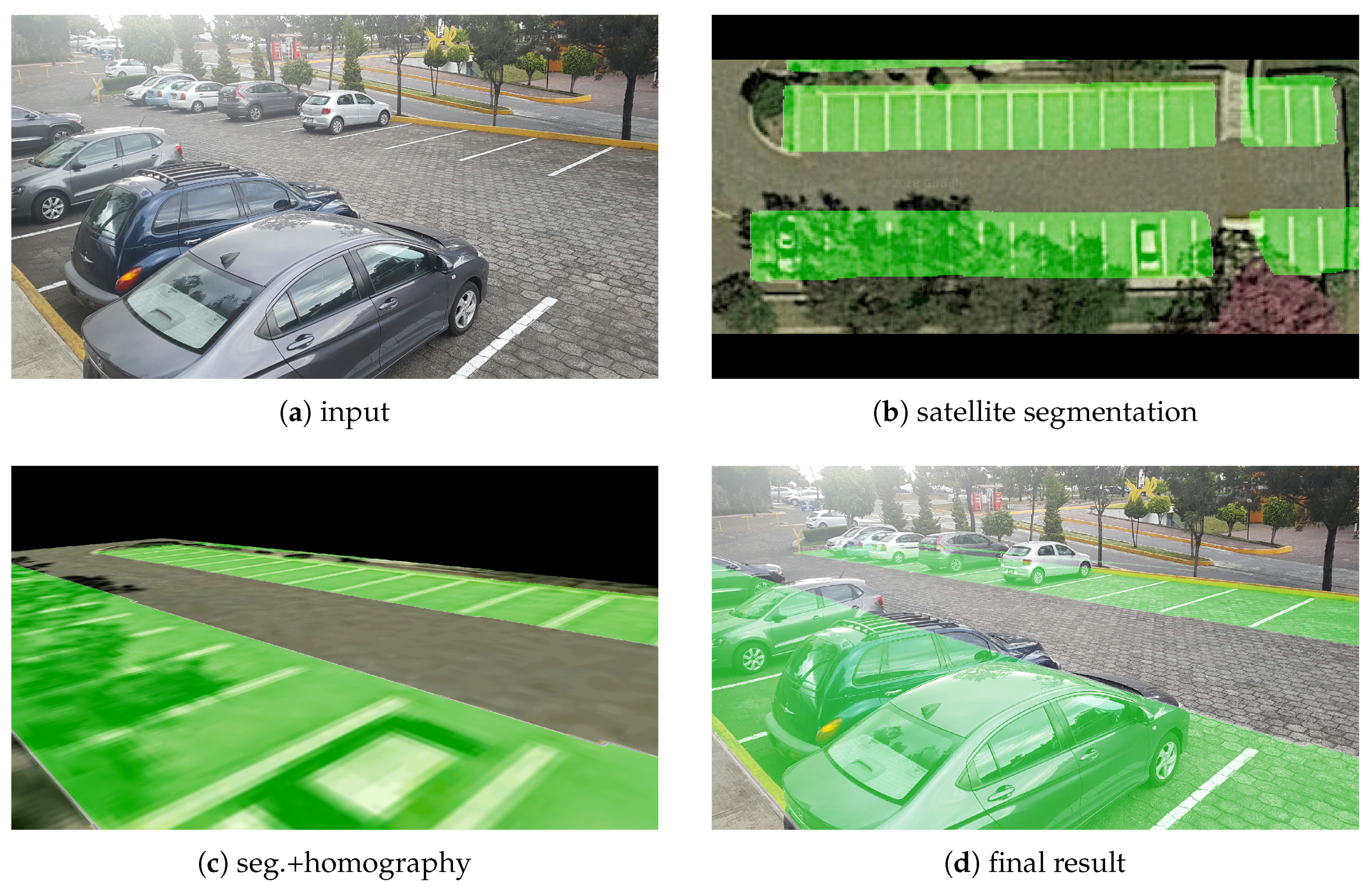
• Segment the parking blocks on the satellite image.
• Calculate an homography between the two perspectives.
• Translate the results of the satellite image into the surveillance camera image.

The beauty of this approach is that it helps us overcome the two main challenges previously mentioned—(1) temporal and static frontal occlusions [8] (It is worth noting that overhead occlusions can be an emerging problem but they are compensated by a clearer shot of the overall parking block structure as we will see later) and (2) variations of the point of view [9] that thwarts a supervised training approach. See Figure 1 for an illustration of our proposal.

Nowadays available datasets are not enough for training a neural network, further on we explain why is this so in the datasets section. Nonetheless, we saw this challenge as a great opportunity to make a contribution to the computer vision field for identifying human made structures from the sky. For the previously mentioned reason—and in particular—to be able to train our image segmentation model in the satellite perspective, we introduce APKLOT, a dataset for direct parking block segmentation from a satellite perspective. More details about APKLOT (APKLOT dataset files are available on the author’s Github account (https://github.com/langheran/APKLOT, Current version: 21 July 2020) dataset will be given in Section 3.

Our image segmentation model was inspired by the publicly available convolutional neural network for image segmentation implementation in dlib [10] with custom parameters. For the homography calculation step we used a custom python tool that helped us mark the correspondence points, even though this wouldn’t be necessary if we had had the physical setup camera projection parameters. These steps will be explained in further detail in the following sections.

Finally, we also propose an evaluation protocol based on the work in Reference [8]. Companion code for all the aforementioned tasks is also provided in the github repository.

The paper is organized as follows. Section “Related Works” explains why this problem is important in the context of the current available related work and the specific way in which we will measure success. Section 2 describes an overview of the method, emphasizing the implemented convolutional neural network and the related works from which our intuition stems. Section 3 presents the dataset we used to train our unique approach to parking block segmentation. Section 4 proposes a set of experiments to evaluate the dataset in the face of the most influential hyperparameters proposed in the literature. It also places each result along the method steps, thus providing a clearer perspective of their contribution. Section 5 remarks on the paper’s most valuable contributions and detours into further developments that can be supported by our work.

Related Works

Most prior work focuses on detecting a global parking lot structure. Of the most prominent examples Huang et al. stands out with a series of works [11,12] that calculate global parameters such as angle to the traffic lane and distance between each parking spot per parking lot.

References [12,13], and more recently Reference [14], all use a two tier combination of vehicle detection with a free (vacant) parking spot detection combination to determine structure global parameter in the parking blocks.

Free parking spot detection and segmentation usually uses human-painted parking lot demarcations. These are ground appearance features that mostly lie on the same plane and are more visible from a high resolution satellite view [15]. They have been exploited extensively in the literature [16]; Mexas and Marengoni [13], for example, using the Hough transform. Other features can be extracted from movement in video [2] and from the spatial distribution of known entities like other cars [17].

Our work addresses the more general problem of extracting the parking lot structure from a single satellite image without making any global shape assumptions. In this way, we are able to detect parking blocks of arbitrary shapes.

Also, most of the prior work focuses on first detecting parking spots and then assembling those instances into a set characterized by a single partition function, that is, a parking block, for example, in References [4,11] they use this approach. With these settings, a considerable chunk of the global information encoded in the image is then dismissed. This information is crucial for detecting partially occluded parking spots.

In contrast, our work does not waste any global information because it takes the pyramidal approach and starts by detecting parking blocks. In this work we do not attempt to detect individual parking spots. However, given the Occam’s razor principle and Joshua Tenenbaum’s size principle (also known as the Occam’s razor principle inspired by the English monk and philosopher William of Occam.) [18] a smaller hypothesis localized only on a single parking block would make global assumptions more consistent with the data.

2. Methodology

Recall that our objective is to segment parking blocks on the surveillance camera perspective. We previously mentioned how satellite views simplify the task of recognizing parking spots. These approaches have been neatly fitted into a two-category taxonomy by Huang [12]—car-driven and space-driven. However, in this work we took a joint approach that detects parking blocks from the camera perspective.

Convolutional neural networks (CNNs) were successfully used to detect parking lot patches from aerial imagery in Reference [19] with a best test classification accuracy of 94.3%. Authors in [20] use a CNN based on AlexNet for occupancy detection over PKLot and their own dataset CNRPark, achieving roughly a 3% overall accuracy improvement compared with previous methods based on two textural descriptors, namely Local Binary Patterns and Local Phase Quantization presented in Reference [9]. The Cityscapes challenge [21] provides segmented parking areas (not necessarily parking blocks). However, Cityscapes does not provide accuracy values for evaluating this class performance and whenever a car or other object is in front, the resulting class is this other object and not the parking area.

One domain from a satellite perspective that is remarkably similar to parking block segmentation is building block segmentation [22,23,24]. In fact, the front page image of Reference [22] shows parking block areas segmented by mistake. This is a clear hint that their method would also perform well on parking blocks, given that our method could be considered a more general case. The best results in both cases were obtained by fully convolutional networks (FCNs) with 88.5% overall accuracy and 0.69 intersection over union (IoU) (XD_XD algorithm on las Vegas) respectively.

Fully convolutional networks are a generalization over CNNs and were introduced by Reference [25]. Given that they don’t have fully connected layers they can manage different input sizes and are faster. U-Net [26] is an improved version of the original FCN that has in the upsampling part a large number of feature channels to better propagate context information to higher resolution layers. In this work we used a modification of U-Net that was implemented by Juha Reunanen and Davis King in Reference [10].

In brief, we use a CNN to segment the parking blocks from an satellite view. Even though it is quite simple, this approach has never been taken in previous works at the time of writing, maybe due to the lack of a dataset that could serve for training.

Recall that our solution proposal consists of using the segmentation of a public satellite image and combine it with the surveillance camera view to generate an extremely accurate segmentation of the surveillance camera, regardless of any temporal or obstacles interfering with camera’s view. An outline of the developed method is given in Algorithm 1. Also, a graphical overview of the proposed method is provided in Figure 2.

Algorithm 1 Parking Block Segmentation from a Surveillance Camera Perspective

Input:$NET$—Pre-Trained CNN    $SAT$—Satellite image    $PMS$—Camera extrinsic parameters Output:$SEG$—Segmented camera-view parking lot 1: procedureSegmentCamera($NET$, $PMS$) 2:   $IMG\leftarrow$ ExtractCameraFrame() 3:   $SAT\leftarrow$ CropScale($SAT$) 4:   if $PMS\equiv Ø$ then 5:    $PMS\leftarrow$ GetExtrinsicParams() 6:   end if 7:   $HOM\leftarrow$ GetHomography($SAT$,$IMG$,$PMS$) 8:   $SSAT\leftarrow$ SegmentSatellite($NET$, $SAT$) 9:   $SEG\leftarrow$ Apply($HOM$,$SSAT$) 10:   return $SEG$ 11: end procedure

▹ Read image from camera ▹ Crop and scale the satellite image   ▹ Get camera parameters   ▹ Get homography from correspondence points ▹ Use ANN to segment satellite image ▹ Apply hom. to segmented satellite image

The first two steps, that is, Figure 2a,b of our proposal in Figure 2 are explained further in Section 3.1. Also the procedure for Figure 2d, in which we collected the surveillance camera images, is included there.

For Figure 2c, the fully convolutional CNN architecture was inspired by the U-Net architecture [26] and implemented by Juha Reunanen and Davis King in Reference [10]. Firstly, we randomly cropped 227 × 227 chips, emulating the same methodology of AlexNet in the ImageNet ILSVRC-2012 challenge [27]. The chips were also randomly horizontally flipped. Then, the input layer was submitted to 220 layers. We also used skip connections in each block as suggested by Reference [28].

3. Dataset

Another contribution of this work is a dataset designed to overcome the limitations of previous datasets like those in References [9,21], mentioned in the Introduction (variations of the point of view and no parking blocks, respectively). In contrast, our method uses the training set of this dataset to adjust the parameters of the CNN from the satellite perspective. Our dataset has roughly 7000 polygons in 500 labeled images. Normally a classical CNN would require much more samples to train, for example AlexNet was trained using 1.2 million training images from ImageNet. By using the fully convolutional architecture implemented by King [10] (based on Ronneberger [26]) we are able to circumvent this requirement and train with only 4034 parking block polygons, that is, 300 images. Ronneberger explains the importance of data augmentation for learning shapes with elastic deformations in their architecture. Taking into consideration Ronneberger’s comments, we augmented 30,000 images from those 300 for a total of 30,300 for the CNN’s training. Our data augmentation consisted in:

• Randomly crop by a value between 0 and 50 pixels
• Horizontally flip 50% of the images
• Vertically flip 50% of the images
• Rotate images by a value between −45 and 45 degrees

Those images are not included in the APKLOT dataset, but we included the data augmentation python code (jittering hereafter) in our repository.

3.1. Image Collection Procedure

APKLOT consists of a total of 500 24-bit RGB images, in both PNG and high-resolution JPG at 96 dpi, with more than 7000 annotated polygons in total. The images were collected first by downloading the coordinates from Open Street Maps. Then, we downloaded the patches containing individual parking lots from google maps using a single zoom level. The parking lots were filtered according to the following conditions:

• They show outdoor parking lots.
• At clear orthogonal daylight, i.e., photos taken in the day, regardless of brightness levels.
• Demarcated using international standards or the ones corresponding to that country for public parking lots.
• Meant to harbor vehicles no larger than full-sized cars (no more than 5350 mm of length).
• Full parking lot view if possible.
• At least a block of 3 parking spots must be visible.

Figure 3 depicts a few instances of parking lots that were analyzed for inclusion in our dataset. Figure 3a,b were both excluded from our dataset given the poor demarcation in the former and poor lighting conditions in the latter. In contrast, Figure 3c was included in our dataset given its high quality in terms of the aforementioned conditions.

Then, on Google Maps, the proper zoom can be calibrated to a specific meters per pixel ratio. In our case we set the zoom level to 20 for 0.1407 m/pixel (roughly 14 cm per pixel) (Please refer to the APKLOT dataset github site in case you would like to use the scripts there to download the google maps images with a different zoom level.)

Cropping was initially made by calculating the bounding box with respect to Google map’s north (without rotation). In some rare cases the image was cropped manually where the resulting image of the initial cropping was too big to fit in the GPU memory, see Section 3.1. Also, the following considerations were applied:

• The resulting image must have the same zoom as the images in the training set, regardless of its width and height.
• The parking space preferably must be on the center of the image.
• Edge structures that do not correspond to parking spots and traffic lanes can be safely excluded.

3.2. Annotated Attributes

The images were annotated by marking the parking block polygons using the labelme tool. Complete parking blocks were annotated i.e., we are not considering the following:

• Parking spots outside the parking lot.
• Badly parked vehicles, including those parked on the traffic lane and non-parking spot (benches, gardens, etc.)
• Debris or machinery in the parking spot when it is used as manner of storage facility.
• Trees in the way of the parking spot.

These annotations where then transformed into the Pascal VOC format (available in its repository). We are also providing the original labelme format.

3.3. Dataset Statistics

Table 1. Image sets in APKLOT.

Year	Statistics	Notes
2018	Only 1 class discriminating between parking spot and other spaces. Train:   300 images   4034 labelme polygons Validation:   100 images   1513 labelme polygons Test:   101 images   1459 labelme polygons	Images were taken from Google Maps API at zoom level 20.

shows the control figures for each of the produced image sets.

Figure 4 shows the general statistics of the input and mask coverage ratio. We can see the annotated class is clearly unbalanced, with only 24.5% corresponding to parking blocks. To overcome this challenge we must select a metric that compensates this phenomenon. In the next section we will see how the IoU metric has been used efficiently in the past for similar cases.

It is also worth mentioning that the parking lot instances have a mean of 15.7 polygons, a maximum of 332 and a minimum of 0. The standard deviation on the number of polygons per parking lot is 26.31.

3.4. Evaluation Protocol

This section describes an evaluation protocol proposed on the basis of the APKLOT dataset. This protocol is the applied further on in the experiments section.

The overall accuracy metric considers the model’s capability of not including some areas in the predicted class, that is, the negative cell on the contingency table. Conversely, recall, precision and the F-Measure are considered to be biased in this sense. In order to avoid this bias, the authors of PKLot [9] and DLib [10] opted to use only overall accuracy. Overall accuracy is given by Equation (1), where $T_p$ are the true positives, $T_n$ are the true negatives, $F_p$ are false positives, $F_n$ are false negatives, P is the sum between true and false positives and N is the sum between true and false negatives. Finally, $Right=T_p+T_n$ and $Wrong=T_p+T_n$.

$$Acc=\frac{T_p+T_n}{P+N}=\frac{T_p+T_n}{T_p+T_n+F_p+F_n}=\frac{Right}{Right+Wrong}.$$

(1)

This metric is usual in cases where we would like to classify individual instances without considering their spatial locality. Yet, the case of pixel segmentation deserves a special consideration. Each pixel is an instance we want to classify. However, most of the features come from the neighboring features. A foreground detected near the ground truth has presumably more informational value than a background detected near the ground truth to such a point that the distinction between foreground and background becomes relevant.

One of the Pascal VOC [8] challenges consists of detecting many classes and marking them by using bounding boxes. Then, the background coincidences play no important role in how to position and scale the bounding boxes over detections. However, the overlapping between the true box and the predicted box is a good indicator of how well the prediction is performing. This overlapping is reflected in Equation (2), that is, the IoU formula proposed by Reference [8].

$$IoU=\frac{T_p}{T_p+F_p+F_n}=\frac{{\bigcap }_{area}}{{\bigcup }_{area}}.$$

(2)

Equation (2) measures the overlapping pixels between the ground truth polygon and the prediction polygon, regardless of the similarity between the areas outside of the polygons. That is, the true negatives are not taken into account. The idea is to reward overlapping foregrounds, instead of backgrounds. An IoU score greater than 0.5 is normally considered a “good” prediction for example, 10 different IoU thresholds are considered from 0.5 to 0.95 in the COCO challenge [29].

4. Experiments and Results

Having reviewed the structure of APKLOT, let us see how it is used in the steps required by the methodology.

It is important to mention that, to our knowledge, no other works on the state-of-the-art deal with the problem of segmenting parking blocks from the camera perspective. The distinction between parking blocks and parking spots is an important one because the former ranges in a variety of non-uniform shapes absent in the latter. Cityscapes [21] includes a label for segmenting parking spots from the camera perspective, but this label is not included in any evaluation and is treated as void. However, if a future work would like to compare their results with ours, they could use pixel-level intersection over union (also used in Cityscapes but for other labels).

In consideration of this void in the domain of parking blocks, we decided to compare the training of the CNN with the original APKLOT dataset to training with an augmented version of the same dataset, that is, the 300 satellite images of the original training set were used to train one set of experiments. In parallel, 100 samples for each of those images were generated to accrue a total of 30,300 sample images for a second set of experiments. In particular the data augmentation that was done consisted in the following actions:

• Randomly crop by a value between 0 and 50 pixels
• Horizontally flip 50% of the images
• Vertically flip 50% of the images
• Rotate images by a value between −45 and 45 degrees

Secondly, testing of the CNN was done with 100 independent satellite view images (hereby __World_). In parallel, 14 independent satellite view images of the Tecnologico de Monterrey (ITESM) were also segmented. These images are the ones we will use to test the algorithm performance once we have translated the results into the 62 surveillance camera images inside ITESM.

Finally, the homographies for each of the 62 surveillance camera perspective images were calculated from the correspondence points and applied to the previous 14 images’ segmentation results. To find the best four points for the homography, we used algebraic error, the default for the OpenCV findHomography method. See Figure 5 for a visual guide to these steps.

Figure 5 shows a tree structure to help us visualize the data flow and metrics used. The yellow diamonds correspond to the main metrics for measuring the contribution of this work. We already explained both overall accuracy and IoU in Section 3.4. Multiclass logistic regression (i.e., negative log-likelihood loss, NLL or categorical cross entropy) is used in tandem with a softmax layer (one-hot) and estimates the maximum a posteriori class label given the parameters learned by the CNN. Each of the dataset icons is captioned with the number of annotated instances contributed. The numbers on the top of each dataset icon represent the number of instances before augmentation and single polygon extraction. 300 parking lots and their polygons to train the CNN, 100 for testing, 14 parking lots inside the university, 62 ground camera view image that correspond to those 14 and a set of more than 4 correspondence points for each of those 62 images.

4.1. Convolutional Neural Networks Setup and Training

In this section we describe the experimental setup, mainly for training the satellite segmentation CNN.

Table 2. Hyperparameter experimental setup.

Hyperparam.	Value	Ab.	Explanation
sample size	300 initial instances and 30,300 instances by augmentation	j	More data is always the best way of reducing the variance without increasing the bias.
batch size	{16,30,32}	b	Using the full instance always gives better accuracy than using a randomly partitioned batch size. However, the model evaluates the full gradient on each epoch and it making it too expensive to train. Using mini batches can ameliorate this problem, although the exact size cannot be taken for granted to be the largest because we are dealing with an stochastic way of partitioning the data. We tuned up this parameter empirically.
initial learning rate	0.1–0.01	l	This value was set taking into account the recommendation of Reference [30]; Smith [31]
minimum learning rate	0.00001–0.000001	r	A smaller learning rate produces more stable hops in the gradient on the seek of optimal weight parameters. Too small learning rate bogs down the convergence speed, though.

shows the hyperparameter values and significance for generating the experiments.

Ancillary techniques were used, such as momentum with weight decay and batch normalization. The values for momentum were set according to [32] (0.9 momentum and ${10}^{-4}$ weight decay). Batch normalization window was set large enough to preserve a maximum convolutional layer of 512.

Finally, the experiments were named using the following naming convention:

<jittering was used>j-<batch size>b-<initial learning rate>l-<minimum learning rate>r

In total, we performed 15 experiments. Twelve of these used the external data augmentation already described in the previous section besides the one that does dlib by default (random cropping and horizontal flipping). The other experiments only used the dlib default data augmentation. In the data augmentation experiments, the initial learning rate was set fixed to 0.1 in contrast to the cases not using data augmentation that also used 0.01. However, batch sizes were cycled equally between the three values 16, 30 and 32.

At the first experiments we found that minimum learning rate was unimportant so the experiments corresponding to a batch size of 32 use only ${10}^{-5}$ in contrast to the 16 and 30 cases that use also a ${10}^{-6}$ minimum learning rate.

During training, we found that models using data augmentation produced a higher negative log likelihood with a p value of 0.6% (Mann-Whitney-U). Also we found that models with a batch size less than 16 had a shorter duration with a p value of 0.4%. The faster model was using rotation jittering, 16 batch size, 0.01 initial learning rate and minimum learning rate of 0.000001. See Figure 6 for a graphic of these results, Figure 6a shows the negative log likelihood and Figure 6b shows the overall durations.

Each of these experiments was tested using a I7 Intel Core with 32 GB of RAM and 11 GB GPU, namely using a NVIDIA GeForce GTX 1080 Ti. Images more than 4,000,000 squared pixels were too big for the GPU and triggered a CUDAMalloc (memory allocation) error.

4.2. Expected Results

Each of the perspectives we used was subject to error sources that could damage our results. On the satellite segmentation step we can have occlusion, objects with very similar texture to parking blocks and no visible parking lines at all. See Figure 7 for a visual reference of these errors.

Cases of Figure 7a,b, that is, when a transparent roof is occluding the parking block and when a grid like roof is near the parking lot, could be solved using a Bayesian approach (like the one used by Huang and Wang [12]) to learn the overall structure of the parking lot and discarding the areas that deviate too much from the learned parameters. Cases when there is no demarcation in the parking lot Figure 7c are a little bit trickier. To solve such a case we would need to change our selection criteria in the dataset and include more images of unmarked but identifiable parking lots without relying on the ground appearance, e.g., by using the parking spatial arrangement.

On the camera perspective we can have resolution mismatch and multilevel parking lots. Figure 8a,b show these errors respectively.

Case Figure 8a could be solved by trivially calculating a linear interpolation of a convex polygon shape. Case Figure 8b could be solved by integrating height data [33] to separate planes in the homography calculation.

4.3. Image Segmentation Results

In this section we present the results from testing both segmentation on the satellite 100 independent images and on the surveillance camera images located at the ITESM. We are presenting both results to allow improvements along the pipeline.

Firstly, in the satellite image segmentation, we achieved more than 50% IoU in all models, shown in Figure 9. Figure 9a shows the results using overall accuracy. This metric achieved a notably higher score than the IoU shown in Figure 9b. Recall that in IoU we are not considering true negatives, just true positives, that is, the non segmented areas in the ground truth have no effect on improving the metric artificially.

The variance of the models can be seen from the standard deviation. The most stable model (less standard deviation) was 0j-16b-0.01l-0.000001r which achieved a median of 88.93 overall accuracy. The model scored second if we order them by the worse segmented example, so this model can be considered the best among those we trained.

Satellite segmentation results on the ITESM images (see Figure 10) had greater variance. Nonetheless, the median remained inside two orders of magnitude of the previous results. The Wilcoxon signed rank test showed that we can reject the null hypothesis that the two medians are the same. There is a significant improvement in the ITESM images using IoU. This could be explained by the absence of roof-like structures in ITESM that can produce a greater number of false positives. Also, parking lots are very well maintained and painted inside the institution in contrast with the World dataset. Counterintuitively, the results are inverted when using overall accuracy and there is a significant difference. We surmise that there are many more true negative areas, meaning empty spaces on the images of the World dataset. Also, given the ITESM location on a top-hill, there is also a lot of variability in the slopes that increase the false positive rate.

Segmentation of the satellite images performed quite well, both at time and accuracy. However, when introducing a homography transformation, the median results dropped, shown in Figure 11. Considering this fact, we can safely conclude that any improvement in the homography calculation will greatly improve the overall result.

All supervised segmentation done in APKLOT follows a clear rule—mark the area wherever is visible. However, one of the known issues of evaluating a supervised segmentation task is that the ground truth data is vulnerable to the subjective criteria of each person [34]. Furthermore, pixel-by pixel segmentation have many challenges like—partial occlusions, tool limitations, resolution mismatches and alike. Considering these natural limitations, perfect accuracy would only be achievable in case the two shapes, that is, the predicted and the ground truth shapes, were identical. To overcome this challenge, we have included the first boxplot of Figure 11 as a baseline. This boxplot shows the results of the satellite ground truth images with the applied homography. Finally, all the boxplots were produced using the real ground truth segmented by a human in the camera perspective. A three-number summary (first and third quartile omitted due to lack of space) of the distribution is given in

Table 3. Segmentation camera results on the ITESM dataset (14 + 62 images).

Parameters	Overall Accuracy					IoU
	Mean	Std	Min	50%	Max	Mean	Std	Min	50%	Max
0j-16b-0.01l-0.000001r	84.5	8.2	49.5	86.5	96.8	57.7	20.1	0.0	62.1	95.2
0j-16b-0.01l-0.00001r	84.9	8.5	50.1	87.5	95.0	57.6	20.4	4.2	60.1	92.7
0j-16b-0.1l-0.000001r	85.7	7.8	50.8	87.3	96.4	59.5	20.0	2.4	62.1	94.7
0j-16b-0.1l-0.00001r	84.7	8.9	50.4	87.2	97.3	57.7	20.3	3.3	59.0	96.0
0j-30b-0.01l-0.000001r	85.0	8.2	50.6	87.0	98.1	58.3	20.5	0.8	59.7	97.0
0j-30b-0.01l-0.00001r	84.5	7.8	53.6	86.3	96.4	57.7	19.7	0.0	60.3	94.6
0j-30b-0.1l-0.000001r	85.2	8.4	50.2	87.6	97.5	58.9	20.3	2.4	59.8	96.2
0j-30b-0.1l-0.00001r	85.1	8.3	49.4	87.3	96.8	58.9	19.6	1.5	60.2	95.1
0j-32b-0.01l-0.00001r	84.5	8.0	52.7	87.0	95.3	57.5	19.8	0.0	60.1	91.7
0j-32b-0.1l-0.00001r	85.2	8.0	50.9	87.3	96.5	59.3	19.9	1.6	61.4	94.8
1j-16b-0.1l-0.000001r	82.7	10.5	45.8	86.5	94.9	53.9	21.3	8.6	59.2	90.5
1j-16b-0.1l-0.00001r	84.0	8.2	59.7	86.6	94.6	56.0	21.1	11.1	58.5	91.7
1j-30b-0.1l-0.000001r	83.6	8.9	51.7	86.3	96.1	56.0	21.1	3.3	59.3	90.2
1j-30b-0.1l-0.00001r	83.8	8.4	54.4	86.4	95.8	56.8	19.0	9.6	59.1	92.3
1j-32b-0.1l-0.00001r	83.8	9.2	51.4	86.7	95.2	56.3	21.1	3.2	60.3	93.0
ground-truth with-homography	88.2	8.8	58.4	91.3	96.7	66.5	20.3	9.2	72.2	92.2

.

Figure 11 shows that the results are pretty low compared with the satellite image segmentation alone. Still, the mean and median IoU remains above 50% so we can consider the results good enough and confirm our hypothesis. Thus, in most cases the error was magnified. Assuming that the homography was perfect and all the points lie on the same projective plane, calculating the homography from the ground truth picture should produce a near perfect score, except for those cases occluded by roof-like structures and resolution mismatch. However, we see from Table 3 that this is clearly not the case, given that the median dropped from 91.3% to 87.6% of the best median for overall accuracy and even a more dramatic drop of 72.2% to 62.1% in the case of IoU.

5. Conclusions and Recommendations

The main focus of this paper was solving the parking block segmentation on a surveillance camera perspective problem by taking advantage of the satellite view of the same scene. The goal of this research was two-fold—firstly, to segment parking blocks on aerial images. Given the non-existence of a proper dataset to accomplish this specific task, we proposed APKLOT, a collection of 7000 parking block polygons that proved to be enough to achieve 50% IoU world wide; secondly, to translate these results to a surveillance camera perspective and measure the ensuing degradation. By testing on several CNNs we provide the groundwork to support the relationship between each hyperparameter, learning rate and duration. We demonstrated that using a simple architecture like the U-Net with skip connections is sufficient to segment simple shapes like the ones composing parking blocks, even though many are heavily occluded.

For future work we recommend learning the homography automatically without relying on explicitly providing the camera projection parameters or the correspondence points. Then, our approach could be applied to any outdoor parking lot without human intervention. For the case of automating the correspondence points extraction, they can be learned using a metric learning approach as proposed in Reference [35].

References

1. Harrell, E. Violent Victimization Committed by Strangers, 1993–2010; Bureau Justice Statistics Special Reports; US Department of Justice: Washington, DC, USA, 2012. [Google Scholar]
2. Sevillano, X.; Mármol, E.; Fernandez-Arguedas, V. Towards smart traffic management systems: Vacant on-street parking spot detection based on video analytics. In Proceedings of the 17th International Conference on Information Fusion (FUSION), Salamanca, Spain, 7–10 July 2014; pp. 1–8. [Google Scholar]
3. Huang, T.; Koller, D.; Malik, J.; Ogasawara, G.; Rao, B.; Russell, S.; Weber, J. Automatic Symbolic Traffic Scene Analysis Using Belief Networks. In Proceedings of the Twelfth National Conference on Artificial Intelligence, 2nd ed.; American Association for Artificial Intelligence: Menlo Park, CA, USA, 1994; pp. 966–972. [Google Scholar]
4. Seo, Y.W.; Ratliff, N.D.; Urmson, C. Self-Supervised Aerial Image Analysis for Extracting Parking Lot Structure. In Proceedings of the International Joint Conferences on Artificial Intelligence IJCAI, Pasadena, CA, USA, 11–17 July 2009; pp. 1837–1842. [Google Scholar]
5. Sastre, R.J.L.; Jimenez, P.G.; Acevedo, F.J.; Bascon, S.M. Computer Algebra Algorithms Applied to Computer Vision in a Parking Management System. In Proceedings of the 2007 IEEE International Symposium on Industrial Electronics, Vigo, Spain, 4–7 June 2007; pp. 1675–1680. [Google Scholar]
6. Weis, T.; May, B.; Schmidt, C. A Method for Camera Vision Based Parking Spot Detection; SAE Technical Paper Series; SAE International: Warrendale, PA, USA, 2006. [Google Scholar]
7. Kabak, M.O.; Turgut, O. Parking spot detection from aerial images. In Stanford University, Final Project Autumn 2010, Machine Learning Course CS229; Stanford University: Stanford, CA, USA, 2010. [Google Scholar]
8. Everingham, M.; Van Gool, L.; Williams, C.K.I.; Winn, J.; Zisserman, A. The Pascal Visual Object Classes (VOC) Challenge. Int. J. Comput. Vis. 2010, 88, 303–338. [Google Scholar] [CrossRef] [Green Version]
9. Almeida, P.R.; Oliveira, L.S.; Britto, A.S.; Silva, E.J.; Koerich, A.L. PKLot—A Robust Dataset for Parking Lot Classification The PKLot Dataset. Expert Syst. Appl. 2015, 42, 1–6. [Google Scholar] [CrossRef] [Green Version]
10. King, D.E. Dlib-ml: A Machine Learning Toolkit. J. Mach. Learn. Res. 2009, 10, 1755–1758. [Google Scholar]
11. Huang, C.C.; Wang, S.J.; Change, Y.J.; Chen, T. A Bayesian hierarchical detection framework for parking space detection. In Proceedings of the 2008 IEEE International Conference on Acoustics, Speech and Signal Processing, Las Vegas, NV, USA, 31 March–4 April 2008; pp. 2097–2100. [Google Scholar]
12. Huang, C.; Wang, S. A Hierarchical Bayesian Generation Framework for Vacant Parking Space Detection. IEEE Trans. Circuits Syst. Video Technol. 2010, 20, 1770–1785. [Google Scholar] [CrossRef]
13. Mexas, A.H.; Marengoni, M. Unsupervised Recognition of Parking Lot Areas. In Proceedings of the International Conference on Machine Vision and Machine Learning, Prague, Czech Republic, 14–15 August 2014. Paper No. 68. [Google Scholar]
14. Koutaki, G.; Minamoto, T.; Uchimura, K. Extraction of Parking Lot Structure from Aerial Image in Urban Areas. Int. J. Innov. Comput. Inf. Control 2016, 12, 371–383. [Google Scholar]
15. Cheng, L.; Tong, L.; Li, M.; Liu, Y. Extracting Parking Lot Structures from Aerial Photographs. Photogramm. Eng. Remote Sens. 2014, 80, 151–160. [Google Scholar] [CrossRef]
16. Jung, H.G.; Kim, D.S.; Yoon, P.J.; Kim, J. Parking Slot Markings Recognition for Automatic Parking Assist System. In Proceedings of the 2006 IEEE Intelligent Vehicles Symposium, Tokyo, Japan, 13–15 June 2006; pp. 106–113. [Google Scholar]
17. Hsieh, M.R.; Lin, Y.L.; Hsu, W.H. Drone-Based Object Counting by Spatially Regularized Regional Proposal Network. In Proceedings of the IEEE International Conference on Computer Vision (ICCV), Venice, Italy, 22–29 October 2017. [Google Scholar]
18. Murphy, K.P. Machine Learning: A Probabilistic Perspective; MIT Press: Cambridge, MA, USA, 2013; pp. 67–72. [Google Scholar]
19. Cisek, D.; Mahajan, M.; Dale, J.; Pepper, S.; Lin, Y.; Yoo, S. A transfer learning approach to parking lot classification in aerial imagery. In Proceedings of the 2017 New York Scientific Data Summit (NYSDS), New York, NY, USA, 6–9 August 2017; pp. 1–5. [Google Scholar]
20. Amato, G.; Carrara, F.; Falchi, F.; Gennaro, C.; Meghini, C.; Vairo, C. Deep learning for decentralized parking lot occupancy detection. Expert Syst. Appl. 2017, 72, 327–334. [Google Scholar] [CrossRef]
21. Cordts, M.; Omran, M.; Ramos, S.; Rehfeld, T.; Enzweiler, M.; Benenson, R.; Franke, U.; Roth, S.; Schiele, B. The Cityscapes Dataset for Semantic Urban Scene Understanding. In Proceedings of the IEEE Conference on Computer Vision and Pattern Recognition (CVPR), Las Vegas, NV, USA, 27–30 June 2016; pp. 3213–3223. [Google Scholar]
22. Marmanis, D.; Wegner, J.D.; Galliani, S.; Schindler, K.; Datcu, M.; Stilla, U. Semantic Segmentation of Aerial Images with an Ensemble of Cnns. Int. Soc. Photogramm. Remote Sens. (ISPRS) Ann. Photogramm. Remote Sens. Spat. Inf. Sci. 2016, 3, 473–480. [Google Scholar]
23. Marmanis, D.; Schindler, K.; Wegner, J.; Galliani, S.; Datcu, M.; Stilla, U. Classification with an edge: Improving semantic image segmentation with boundary detection. Int. Soc. Photogramm. Remote Sens. (ISPRS) J. Photogramm. Remote Sens. 2018, 135, 158–172. [Google Scholar] [CrossRef] [Green Version]
24. Demir, I.; Koperski, K.; Lindenbaum, D.; Pang, G.; Huang, J.; Basu, S.; Hughes, F.; Tuia, D.; Raska, R. Deepglobe 2018: A challenge to parse the earth through satellite images. In Proceedings of the 2018 IEEE/CVF Conference on Computer Vision and Pattern Recognition Workshops (CVPRW), Salt Lake City, UT, USA, 18–22 June 2018; pp. 172–181. [Google Scholar]
25. Long, J.; Shelhamer, E.; Darrell, T. Fully Convolutional Networks for Semantic Segmentation. In Proceedings of the IEEE Conference on Computer Vision and Pattern Recognition (CVPR), Boston, MA, USA, 7–12 June 2015; pp. 3431–3440. [Google Scholar]
26. Ronneberger, O.; Fischer, P.; Brox, T. U-net: Convolutional networks for biomedical image segmentation. In International Conference on Medical Image Computing and Computer-Assisted Intervention; Springer: Cham, Switzerland, 2015; pp. 234–241. [Google Scholar]
27. Krizhevsky, A.; Sutskever, I.; Hinton, G.E. ImageNet Classification with Deep Convolutional Neural Networks. In Advances in Neural Information Processing Systems 25; Pereira, F., Burges, C.J.C., Bottou, L., Weinberger, K.Q., Eds.; Curran Associates, Inc.: New York, NY, USA, 2012; pp. 1097–1105. [Google Scholar]
28. He, K.; Zhang, X.; Ren, S.; Sun, J. Identity Mappings in Deep Residual Networks. In European Conference on Computer Vision (ECCV); Leibe, B., Matas, J., Sebe, N., Welling, M., Eds.; Springer International Publishing: Cham, Switzerland, 2016; pp. 630–645. [Google Scholar]
29. Lin, T.Y.; Maire, M.; Belongie, S.; Hays, J.; Perona, P.; Ramanan, D.; Dollár, P.; Zitnick, C.L. Microsoft coco: Common objects in context. In European Conference on Computer Vision; Springer: Cham, Switzerland, 2014; pp. 740–755. [Google Scholar]
30. Bengio, Y. Practical recommendations for gradient-based training of deep architectures. In Neural Networks: Tricks of the Trade; Springer: Cham, Switzerland, 2012; pp. 437–478. [Google Scholar]
31. Smith, L.N. Cyclical learning rates for training neural networks. In Proceedings of the 2017 IEEE Winter Conference on Applications of Computer Vision, Santa Rosa, CA, USA, 24–31 March 2017; pp. 464–472. [Google Scholar]
32. Sutskever, I.; Martens, J.; Dahl, G.; Hinton, G. On the importance of initialization and momentum in deep learning. In Proceedings of the 30th International Conference on Machine Learning, Atlanta, GA, USA, 17–19 June 2013; pp. 1139–1147. [Google Scholar]
33. Wang, X.; Hanson, A.R. Parking lot analysis and visualization from aerial images. In Proceedings of the Fourth IEEE Workshop on Applications of Computer Vision, Princeton, NJ, USA, 19–21 October 1998; pp. 36–41. [Google Scholar]
34. Zhang, H.; Fritts, J.E.; Goldman, S.A. Image segmentation evaluation: A survey of unsupervised methods. Comput. Vis. Image Underst. 2008, 110, 260–280. [Google Scholar] [CrossRef] [Green Version]
35. Altwaijry, H.; Trulls, E.; Hays, J.; Fua, P.; Belongie, S. Learning to Match Aerial Images With Deep Attentive Architectures. In Proceedings of the IEEE Conference on Computer Vision and Pattern Recognition (CVPR), Las Vegas, NV, USA, 27–30 June 2016; pp. 3539–3547. [Google Scholar]
Figure 1. Segmented parking blocks despite several frequent vehicle occlusions from a surveillance camera perspective.
Applsci 10 05364 g001
Figure 2. Our Proposal. First, a satellite photo perspective of the same parking area (a) is cropped and scaled (b). The image is then segmented by a pre-trained Convolutional Neural Network (CNN) residual network (c). In parallel, a new frame is taken by the surveillance camera (d). With the help of correspondence or coordinate points previously calculated, the homography between the new surveillance camera image and the satellite perspective (e) is calculated. The homography is then applied to extrapolate the satellite CNN segmentation to the surveillance camera image (f). Red overlay stands for false negatives, blue for false positives and green for true positives.
Applsci 10 05364 g002
Figure 3. Parking lot examples from satellite perspective: (a,b) were both excluded from our dataset given the poor demarcation in the former and poor lighting conditions in the latter. In contrast, (c) is a great example that was included in our dataset.
Applsci 10 05364 g003
Figure 4. Size and sparsity statistics of the input images. (a) depicts width and height distribution of the parking lot satellite images; (b) contrasts total area of the images (left) vs. parking block polygons area (right).
Applsci 10 05364 g004
Figure 5. APKLOT dataflow between training, testing and translating the results to the surveillance camera image. The proposed metrics for measuring success are shown below each step. These metrics are discussed under the Evaluation Protocol section (Section 3.4).
Applsci 10 05364 g005
Figure 6. Average loss and duration are the main features we used for measuring progress and are show here. From (a) we can see that the possibility of reaching the 5000 steps without progress limit inasmuch as average loss increases. From the overall durations in (b) we appreciate that the maximum duration is only about 19 and a half hours. The experiments were named according to the following naming convention: <jittering was used>j-<batch size>b-<initial learning rate>l-<minimum learning rate>r.
Applsci 10 05364 g006
Figure 7. Parking lot examples from the satellite perspective in which our method is prone to fail: (a) transparent roof, (b) grid like roof, (c) no visible demarcation lines. Red overlay stands for false negatives, blue for false positives and green for true positives.
Applsci 10 05364 g007
Figure 8. Parking lot examples from a camera perspective in which our method is prone to fail: (a) resolution mismatch, (b) multilevel parking lot. Red overlay stands for false negatives, blue for false positives and green for true positives. A red outline is shown around the aforementioned problems.
Applsci 10 05364 g008
Figure 9. Segmentation satellite results on the World dataset (100 images): (a) is by using dlib’s measure—overall accuracy, (b) shows intersection over union (IoU). The bests model considering the medians (the mean is vulnerable to outliers) are for (a) 1j-30b-0.1l-0.000001r and for (b) 0j-16b-0.1l-0.00001r. The experiments were named according to the following naming convention: <jittering was used>j-<batch size>b-<initial learning rate>l-<minimum learning rate>r.
Applsci 10 05364 g009
Figure 10. Segmentation satellite results on the ITESM dataset (14 images): (a) is by using dlib’s measure–overall accuracy, (b) shows IoU. The bests model considering the medians (the mean is vulnerable to outliers) are for (a) 1j-30b-0.1l-0.000001r and for (b) 0j-16b-0.1l-0.00001r. The experiments were named according to the following naming convention: <jittering was used>j-<batch size>b-<initial learning rate>l-<minimum learning rate>r.
Applsci 10 05364 g010
Figure 11. Segmentation camera results on the ITESM dataset (14 + 62 images): (a) is by using dlib’s measure—overall accuracy, (b) shows IoU. The bests model considering the medians (the mean is vulnerable to outliers) are for (a) 0j-30b-0.1l-0.000001r and for (b) 0j-16b-0.01l-0.000001r. Satellite ground truth homography transformation to the camera perspective is provided for reference. The experiments were named according to the following naming convention: <jittering was used>j-<batch size>b-<initial learning rate>l-<minimum learning rate>r.
Applsci 10 05364 g011