Unsupervised Deep Learning-Based RGB-D Visual Odometry

Abstract

Recently, deep learning frameworks have been deployed in visual odometry systems and achieved comparable results to traditional feature matching based systems. However, most deep learning-based frameworks inevitably need labeled data as ground truth for training. On the other hand, monocular odometry systems are incapable of restoring absolute scale. External or prior information has to be introduced for scale recovery. To solve these problems, we present a novel deep learning-based RGB-D visual odometry system. Our two main contributions are: (i) during network training and pose estimation, the depth images are fed into the network to form a dual-stream structure with the RGB images, and a dual-stream deep neural network is proposed. (ii) the system adopts an unsupervised end-to-end training method, thus the labor-intensive data labeling task is not required. We have tested our system on the KITTI dataset, and results show that the proposed RGB-D Visual Odometry (VO) system has obvious advantages over other state-of-the-art systems in terms of both translation and rotation errors.

1. Introduction

Visual Odometry (VO) is the process of estimating the position and orientation of a robot or an agent by analyzing continuous camera images [1]. With the VO, positioning can be performed in an environment without prior information. Up to now, VO has been widely applied to various mobile robotic platforms, visual and augmented reality, and wearable devices [2]. The performance of a VO system is determined by several factors, e.g., accuracy, time complexity, robustness, etc.

Traditional VO systems deploy a classic feature-based pipeline, i.e., image correction, feature extraction, feature matching, transformation matrix estimation, and pose graph optimization. Recent VO systems [3,4,5,6] start to deploy deep learning frameworks, some of which have already shown promising results and aroused great interest in the robotics and computer vision domains. Most deep learn-based VO systems use supervised training models, which means we need to deploy ground truth camera poses during training. In order to obtain ground truth data, a lot of manpower, material resources, and time are required. Therefore, some researchers [7,8,9,10] have proposed VO systems based on unsupervised learning, which does not rely on ground truth data. In this way, training data can be easily obtained. In addition, the pose estimation accuracy can be further increased by training with unlabeled datasets which are significantly larger and widely available.

All of the unsupervised methods mentioned above are monocular VO systems which are easy and cheap to set up. However, systems using only monocular images are incapable of recovering absolute scale. Prior or external information has to be introduced for scale recovery. Prior information directly provides a Euclidean distance to VO systems, e.g., mounting a camera on a car at a fixed height [11]. However, the system will inevitably generate noise due to car bumps. Some systems integrate monocular images with multiple other data sources, e.g., Inertial Measurement Unit (IMU) [12], omnidirectional camera [13], stereo camera [14], etc. In the last decade, range-sensing devices have been widely used in various applications, such as self-driving cars, somatosensory games, and even smartphones. Thus, RGB-D data is easily acquirable. This combination has been adopted by many researchers [15,16,17] and normally yields a performance boost.

In our previous work [10], the VO system is a monocular one and adopts a single-channel neural network structure. In this paper, the RGB-D camera is used to provide the system with RGB images and depth images at the same time. The depth images inject absolute scale information, and both of them occupy the same position in the system. During neural network training and pose estimation, a dual-stream neural network is proposed to process RGB images and depth images. Figure 1 shows the proposed system. Our experimental results indicate that adding additional depth streams has impacts on the accuracy and time complexity of the VO system. On one hand, the translation and rotation errors are greatly reduced and the accuracy can be compared to a stereo VO system. On the other hand, the operating speed of the system has slightly decreased.

The system benefits from an unsupervised training framework, under which ground-truth poses in any form are not required for training. During training, transformation matrices generated by the network are used for loss calculation. During testing, consecutive RGB-D images are fed into the network which directly yields poses on an absolute scale. Then, the translation error and rotation error of the system are obtained by comparing the poses of our system with the ground-truth poses. Experiments have been carried out on the KITTI odometry dataset [18] and results have shown that our VO system outperforms other state-of-the-art VO systems in terms of both translation and rotation accuracy. The additional depth information can reduce the pose estimation errors by more than half.

In this paper, we review recent literature on visual odometry in Section 2. Section 3 details the proposed VO system and the implementation method. Experimental results including comparison with other VO systems are presented in Section 4. Finally, we conclude our work and propose ideas for our future research.

2. Relate Works

Visual odometry solves the problem of estimating the trajectory of a robot by using associated camera images as the main input source. The term was introduced by Nistér et al. [1] in 2004 and has attracted enormous attention from computer science and robotics domains. The sensors of the VO system are mainly cameras, and currently, the mainstream ones are monocular cameras [19], stereo cameras [20], and omnidirectional cameras [21]. The monocular VO system has a simple structure, low cost and easy deployment, but it cannot provide absolute scale information [22]. The binocular camera can obtain absolute scale information by calculating the parallax between the two cameras, but it will consume a lot of computer resources for calculation. On this basis, some scholars proposed to integrate other external sensors, such as IMU [23] and Lidar [24,25] into VO systems, and improve their performance through multi-sensor fusion technique. On the other hand, the RGB-D camera can obtain both image and depth information based on structured light or time of flight (TOF) techniques [26]. With the advent of low-budget RGB-D sensors such as Kinect, ASUS Xtion, and Intel SR300 [27], the combination of monocular images and depth information becomes increasingly popular. Traditional RGB-D odometry systems [28] deploy a feature-based pipeline. Image features such as Scale Invariant Feature Transform (SIFT), Speeded Up Robust Features (SURF), and Oriented Fast and Rotated Brief (ORB) are first extracted. Descriptor matching, Random Sample Consensus (RANSAC) and bundle adjustment are commonly used for motion estimation. Associated depth information is then used to inject the absolute scale. Huang et al. [29] applied such system to 3D flight in cluttered environments. Steinbrücker et al. [30] proposed an energy-based approach as an alternative, which infers odometry with dense RGB-D images. The same idea was also adopted by Kerl et al. [15], who minimized both photometric and depth errors over all pixels. Generally, the structures and parameters of these methods need to be carefully designed and fine-tuned to achieve optimal performance.

Recently, attention has been drawn to deep neural networks which have shown remarkable results in most computer science related tasks [31]. These VO systems deploy an end-to-end training approach, i.e., little or no pre-processing on input images and directly output transformation matrices. Networks that are originally designed for other recognition or classification tasks are always leveraged since the features extracted by lower layers of a particular network are transferable. The landmark network, PoseNet [3], proposed by Kendall et al. first applied Convolutional Neural Networks (CNN) to visual odometry. PoseNet takes monocular images as input and directly outputs a 7-dimensional pose vector representing position and direction in real time, which relies on GoogLeNet [32] architecture. GoogLeNet, pre-trained on ImageNet and Places datasets, is modified for this task, in which softmax classifiers are removed and a fully connected layer is inserted. Li et al. [33] improved PoseNet by introducing depth information as the second stream of the network. Wang et al. [34] further extended the CNN-based PoseNet by incorporating a Recurrent Neural Network (RNN) into their system. The CNN is used to extract features across space, while the RNN is used to match features across time. However, these systems require labeled ground truth camera poses to train the neural networks, which is labor-intensive and time-consuming.

Zhou et al. [7] started a research based on an unsupervised framework and proposed a network for monocular depth estimation, which can also be used to output camera poses. This started a research boom based on unsupervised VO systems. However, since the absolute scale information cannot be obtained using only a monocular camera, subsequent processing must be performed on the obtained camera pose. Mahjourian et al. [9] also presented an unsupervised framework using 3D geometric constraints, which is similar to the Iterative Closest Point (ICP) technique. Liu et al. [10] proposed an unsupervised monocular visual odometry system. The system still needs depth information for training. Therefore, we incorporate the additional depth information into our system for both network training and pose estimation to inject absolute scale and meanwhile, boost the pose estimation accuracy. In contrast to recent researches [8,10,33], this paper focuses on additional depth information and further discusses the advantages and disadvantages of adding additional depth information.

3. The Proposed Approach

In this section, we first introduce the structure of our proposed VO system and explain the role of each unit. Then the loss function for neural network training is proposed.

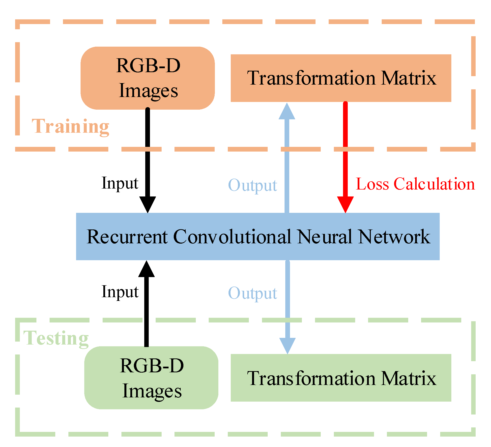
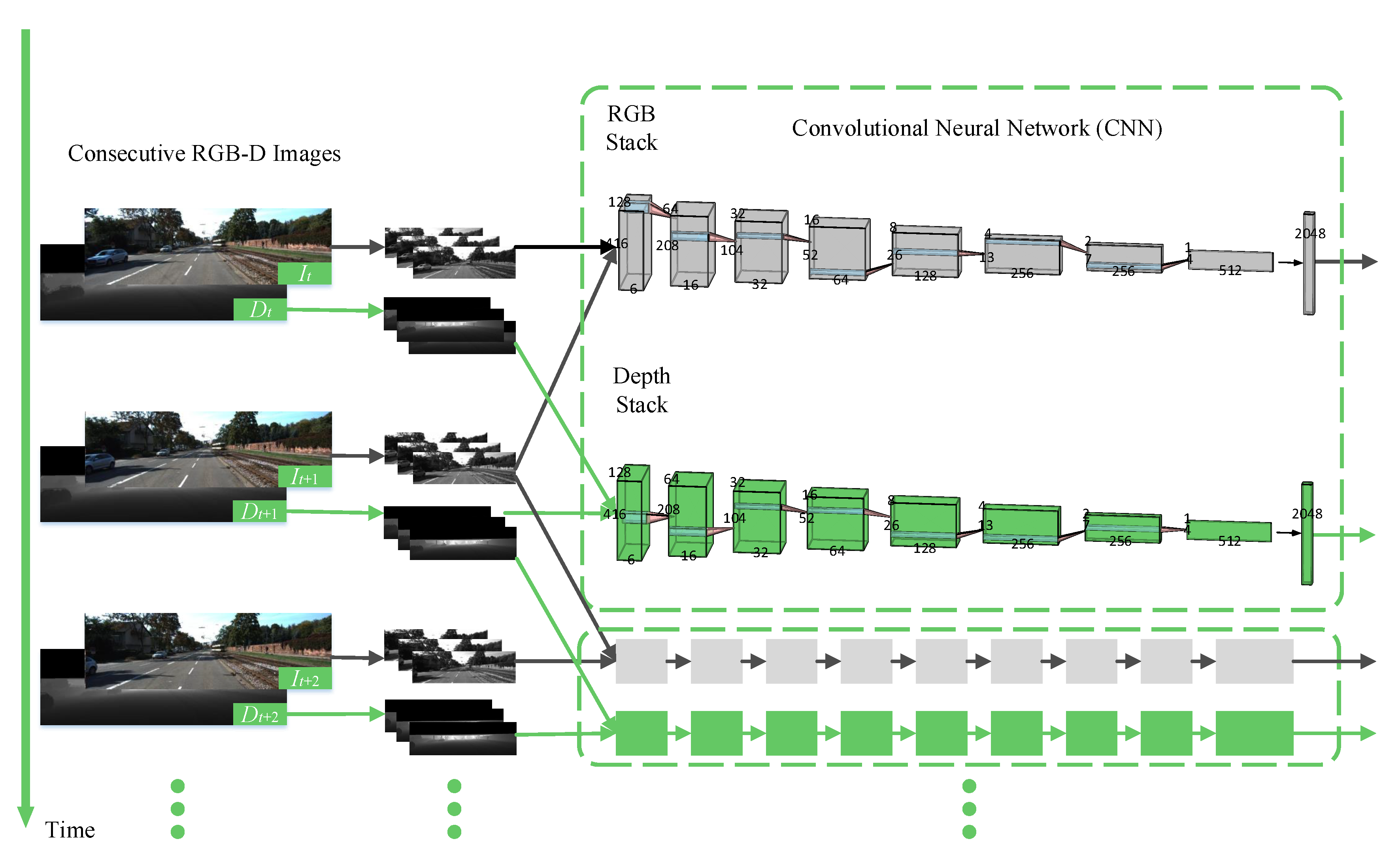
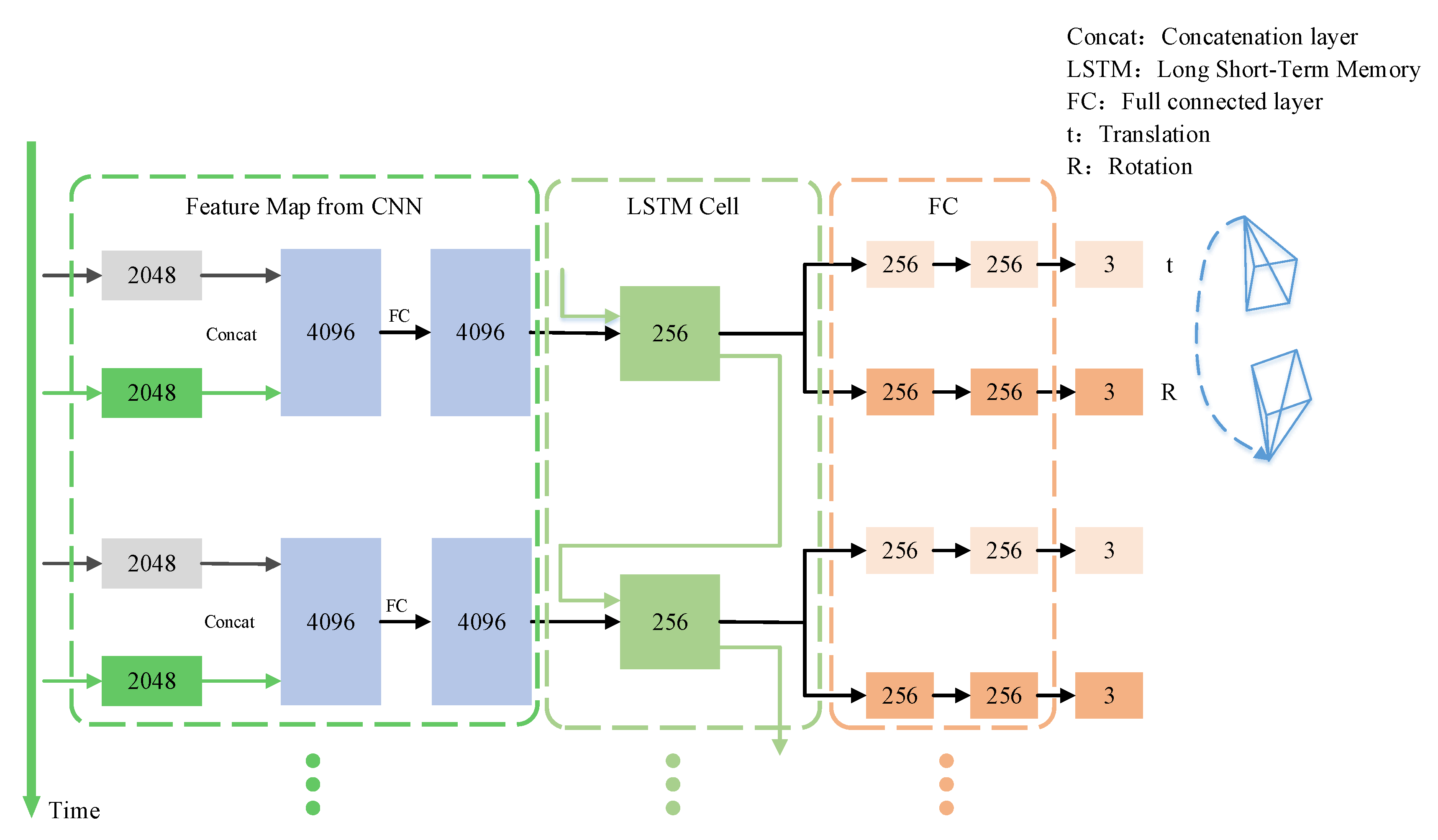
3.1. System Architecture

In this paper, We further adopt the method presented in [34], which combines the advantages of CNN and RNN into a Recurrent Convolutional Neural Network (RCNN). Since VO is the process of estimating a camera’s pose through changes between consecutive frames, the input of the CNN is fused by sequences of adjacent image frames. In addition, in order to inject absolute scale information, we also feed the depth images into the network. The RGB images and depth images have the same CNN network structure. Figure 2 shows the network architecture of the front-end dual-stream CNN, which extracts image features from the RGB stream and the depth stream, respectively. The additional depth channel is highlighted in green. Each time, two consecutive frames of RGB-D image pairs are used for training. Regarding RGB images, we adjust it to $416\times 128\times 3$ along its color channel and then stack consecutive frames together to $416\times 128\times 6$. In terms of the depth image, we first convert it from a 3D point cloud to a single-channel 2D depth image, in which each pixel represents the distance from the viewpoint to the scene object. We then duplicate its single channel to a 3-channel depth image and stack it with the ones of the adjacent frame as $416\times 128\times 6$. The RGB stream and the depth stream form a dual-stream CNN structure. The gray cuboids and the green cuboids in Figure 2 represent the RGB stream and the depth stream, respectively.

The design of the CNN is based on the network developed by Oxford’s Visual Geometry Group (VGG) [35]. We modify the VGG model to fit the VO system proposed in this paper. Both the RGB stream and the depth stream of the CNN begin with a $7\times 7$ convolutional layer, followed by a $5\times 5$ convolutional layer, both of which are used to capture basic components in RGB-D images. The size of the rest 5 convolutional layers is then reduced to $3\times 3$ to capture fine detailed local features. Since the size of input images is relatively small, there is no need to use a big stride to fast reduce the image dimension. In the proposed network, the stride we use is 2. Zero-padding is also deployed to prevent the reduction in image size going too fast. The padding size drops along with kernel size. A Rectified Linear Unit (ReLU) activation function follows each convolutional layer to introduce non-linearity to the network. The conventional batch normalization is not applied in our system since it results in slow and unstable loss convergence during our experiments.

Table 1. Architectures of convolutional layers.

Layer	Conv1	Conv2	Conv3	Conv4	Conv5	Conv6	Conv7
Filter Size	$7\times 7$	$5\times 5$	$3\times 3$	$3\times 3$	$3\times 3$	$3\times 3$	$3\times 3$
Stride	2	2	2	2	2	2	2
Padding	3	2	1	1	1	1	1
Channel Number	16	32	64	128	256	256	512

shows the filter size, stride, padding, and channel number of each convolutional layer in detail. After the dual-stream CNN outputs $4\times 1\times 512$ RGB features and $4\times 1\times 512$ depth features, they are finally reshaped and tiled onto two 2048-dimensional feature vectors. In this way, the absolute scale information is captured by the neural network through the additional depth channel.

The rear-end RNN, as shown in Figure 3, can be viewed as a pose estimator across the whole image sequence. Firstly, a concatenation layer is used to join the RGB and depth feature vectors together. A fully connected layer is followed to balance the weights of these two features. The feature vectors are then ready for the RNN. Since the current inference is highly dependent on the previously estimated position and orientation, we apply RNN to learn patterns of the entire input image sequence. In this case, the use of standard RNN will have long-term dependence problems. Therefore, we use Long Short-Term Memory (LSTM) to replace the standard RNN in our system.

An LSTM unit is composed of a cell and three regulators, namely input, output and forget gate. The cell remembers values over certain time intervals and the three gates regulate the flow of information into and out of the cell, which is the key to an LSTM unit and is shown by the green arrows in Figure 3. The number of hidden units of the LSTM unit is 256, and no projection layer is applied. The biases of the forget gate is recommended to be 1 according to [36].

The vectors generated by the RNN contain rich transformation information within the sequence of images. Most deep learning-based VO systems [7,34] output translation and rotation as a single vector. In contrast, based on the characteristic that rotation generally has higher nonlinearity than translation, we separate the rotation information and translation information into two independent vectors [37]. We then feed the two independent vectors into fully connected layers with dimension 256, followed by an activation function of exponential linear unit (ELU). The final output is a 3D translation vector of Euclidean space and a rotation vector represented by the Euler angle.

3.2. Loss Function

The RCNN generates estimated rotation and translation vectors from pairs of RGB-D images [38]. In order to compare the difference between these output values and true values and drive the predicted results closer to true values, we need to design a loss function. The loss function here consists of two parts: 2D space loss and 3D space loss, which are calculated by RGB-D sequences and the predicted transformation matrices. Algorithm 1 shows the overall architecture in detail.

Let $I_1,I_2,\dots ,I_t,I_{t+1},\dots ,I_N$ be a batch of RGB images ordered by time sequence, $D_1,D_2,\dots ,D_t,D_{t+1},\dots ,D_N$ be the corresponding depth images and $Q_1,Q_2,\dots ,Q_t,Q_{t+1},\dots ,Q_N$ be the point clouds which are back-projected from depth images. Figure 4 shows the loss function calculation process. RGB-D images at time t and $t+1$ generate a predicted transformation matrix ${\widehat{T}}_{t,t+1}$ through the RCNN. All pixels in image $I_t$ are processed according to $D_t$, ${\widehat{T}}_{t,t+1}$ to obtain image ${\widehat{I}}_{t+1}$. The 2D space loss describes the difference between $I_{t+1}$ and ${\widehat{I}}_{t+1}$. As for 3D space loss, its calculation method is similar to 2D space loss, which projects all points in the point cloud $Q_t$ to ${\widehat{Q}}_{t+1}$, through the transformation matrix ${\widehat{T}}_{t,t+1}$. The difference between $Q_{t+1}$ and ${\widehat{Q}}_{t+1}$ is the 3D space loss.

Algorithm 1: Implementation of the RCNN and loss functions.

3.2.1. 2D Spatial Loss

Let $p_t$ be a pixel in the RGB image $I_t$, and $P_t$ be the point in the 3D space corresponding to $p_t$. According to the pinhole camera model, the relationship between them can be described as

$$P_t=d_t{K}^{-1}{p}_t$$

(1)

where $d_t$ is the corresponding depth value of the pixel point $p_t$ in the depth image $D_t$ and K is the camera intrinsic matrix.

Then, based on the transformation relationship of the 3D space coordinate system, the transformation matrix ${\widehat{T}}_{t,t+1}$ obtained by the RCNN network is used to predict point ${\widehat{P}}_{t+1}$ at time $t+1$. ${\widehat{P}}_{t+1}$ can be calculated by

$${\widehat{P}}_{t+1}={\widehat{R}}_{t,t+1}{d}_t{K}^{-1}{p}_t+{\widehat{t}}_{t,t+1}$$

(2)

where ${\widehat{R}}_{t,t+1}$ and ${\widehat{t}}_{t,t+1}$ are rotation matrix and translation vector, respectively, which can be derived from the transformation matrix ${\widehat{T}}_{t,t+1}$.

Next, according to the pinhole camera model, the predicted point ${\widehat{P}}_{t+1}$ is converted back into a predicted RGB image ${\widehat{I}}_{t+1}$ by

$${\widehat{p}}_{t+1}=\frac{1}{{\widehat{d}}_{t+1}}K({\widehat{R}}_{t,t+1}{d}_t{K}^{-1}{p}_t+{\widehat{t}}_{t,t+1})$$

(3)

where ${\widehat{d}}_{t+1}$ is the z-axis coordinate value of ${\widehat{P}}_{t+1}$, which is also the depth value of the pixel point ${\widehat{p}}_{t+1}$.

We perform the above calculation on each pixel in RGB image $I_t$ to obtain the predicted RGB image ${\widehat{I}}_{t+1}$. Regarding the pixels with null values, we use bilinear interpolation to estimate them.

Using the same method, we can get ${\widehat{I}}_t$ by

$${\widehat{p}}_t=\frac{1}{{\widehat{d}}_t}K({\widehat{R}}_{t+1,t}{d}_{t+1}{K}^{-1}{p}_{t+1}+{\widehat{t}}_{t+1,t})$$

(4)

where ${\widehat{p}}_t$ is a pixel in ${\widehat{I}}_t$, ${\widehat{R}}_{t+1,t}$, ${\widehat{t}}_{t+1,t}$ are the rotation matrix and translation vector, which can be obtained by the transformation matrix ${\widehat{T}}_{t+1,t}$, the relationship between ${\widehat{T}}_{t+1,t}$ and ${\widehat{T}}_{t,t+1}$ can be described as

$${\widehat{T}}_{t+1,t}={\widehat{T}}_{t,t+1}^{-1}$$

(5)

Finally, the 2D spatial loss is derived by

$$L_2=\sum _{t=1}^{N-1}\left(\overline{|I_t-{\widehat{I}}_t|}+\overline{|I_{t+1}-{\widehat{I}}_{t+1}|}\right)$$

(6)

3.2.2. 3D Spatial Loss

The difference between the predicted value and the true value is calculated in 3D space. Let $Q_t,Q_{t+1}$ be the point clouds of the depth images $D_t,Q_{t+1}$ back-projected into the 3D space, and $q_t,q_{t+1}$ are the corresponding points in $Q_t,Q_{t+1}$. Based on the transformation relationship of the 3D space coordinate system, we have

$${\widehat{q}}_{t+1}={\widehat{R}}_{t,t+1}{q}_t+{\widehat{t}}_{t,t+1}$$

(7)

where ${\widehat{R}}_{t,t+1}$ and ${\widehat{t}}_{t,t+1}$ are rotation matrix and translation vector, which can be derived from the transformation matrix ${\widehat{T}}_{t,t+1}$. By calculating each point in the point cloud, a predicted point cloud ${\widehat{Q}}_{t+1}$ at time $t+1$ is constructed.

Similarly, the point cloud image ${\widehat{Q}}_t$ at time t can be constructed. Then, the Iterative Closest Point (ICP) [39] method is used to match the points in the point cloud images $Q_t$ and ${\widehat{Q}}_t$, $Q_{t+1}$ and ${\widehat{Q}}_{t+1}$. The 3D space loss can be described as

$$L_3=\sum _{t=1}^{N-1}\left(\overline{|Q_t-{\widehat{Q}}_t|}+\overline{|Q_{t+1}-{\widehat{Q}}_{t+1}|}\right)$$

(8)

Finally, let ${\alpha }_2$ and ${\alpha }_3$ be the weight of 2D space loss and 3D space loss, the total loss function can be derived as

$$L={\alpha }_2{L}_2+{\alpha }_3{L}_3$$

(9)

4. Experiments

We present our experiments in this section. We first introduce our training strategy and network hyperparameters. We then conduct a quantitative and qualitative evaluation on translation and rotation errors of the proposed VO system compared to other state-of-the-art VO systems, namely SfMLearner [7], UnMono [10], and VISO2-Stereo [39]. Finally, the advantages and disadvantages of our proposed VO system are discussed in terms of accuracy and time complexity.

4.1. Training

We implemented our code using Google ’s open source machine learning software library, TensorFlow and completed training on a DELL desktop with an Intel Core i7-4790K @4.0GHz CPU and an Nvidia GeForce GTX Titan X 12GB Memory GPU (Xiamen, China).

We used KITTI [18] Visual Odometry Datasets for training and testing. KITTI Odometry consists of 22 video sequences captured by driving around a midsize city, in rural areas, and on highways. Sequence 00–10 are provided with ground truth for quantitative analysis, whereas sequence 11–21 are used for qualitative analysis. In order to compare with SfMLearner and UnMono, all images are resized to $416\times 128\times 3$ before feeding into the neural network. Because the training data set is relatively small, we have deployed online data augmentation. Through the following steps, we artificially created more training images.

• We randomly adjusted the RGB image brightness by gamma adjustment, and the value range of the encoding/decoding gamma value is $\gamma \in [0.7,1.3]$. Depth images were not processed.
• We randomly adjusted the size of image pairs. The scale factors of the x and y axes are $s_x,s_y\in [1.0,1.2]$.
• Based on the center of an image, the image pairs were randomly rotated, and the rotation angle $r\in [-5,5]$ degrees.
• Based on the image center, the excess part of image was removed and the missing part was interpolated. Finally the image size were adjusted to $416\times 128$.

After data preparation, RGB-D images were fed into the network for training. Thanks to the framework of unsupervised deep learning, the ground truth provided by sequence 00–10 were not used for training, but for performance evaluation. The batch size was 32, and the number of RGB-D images in each batch (sequence) was 5. In order to better complete the training, we deployed the Adam adaptive learning rate optimizer [40] and set the exponential decay rates for the first and second moment estimates ${\beta }_1=0.9$ and ${\beta }_2=0.999$, respectively. The RCNN iterated for 40 epochs, and the total loss usually stabilized after 20 epochs. The subsequent iteration epochs were applied to fine-tune the network. Thus we decreased the learning rate from the initial value 0.0002 to 0.0001 after half training epochs.

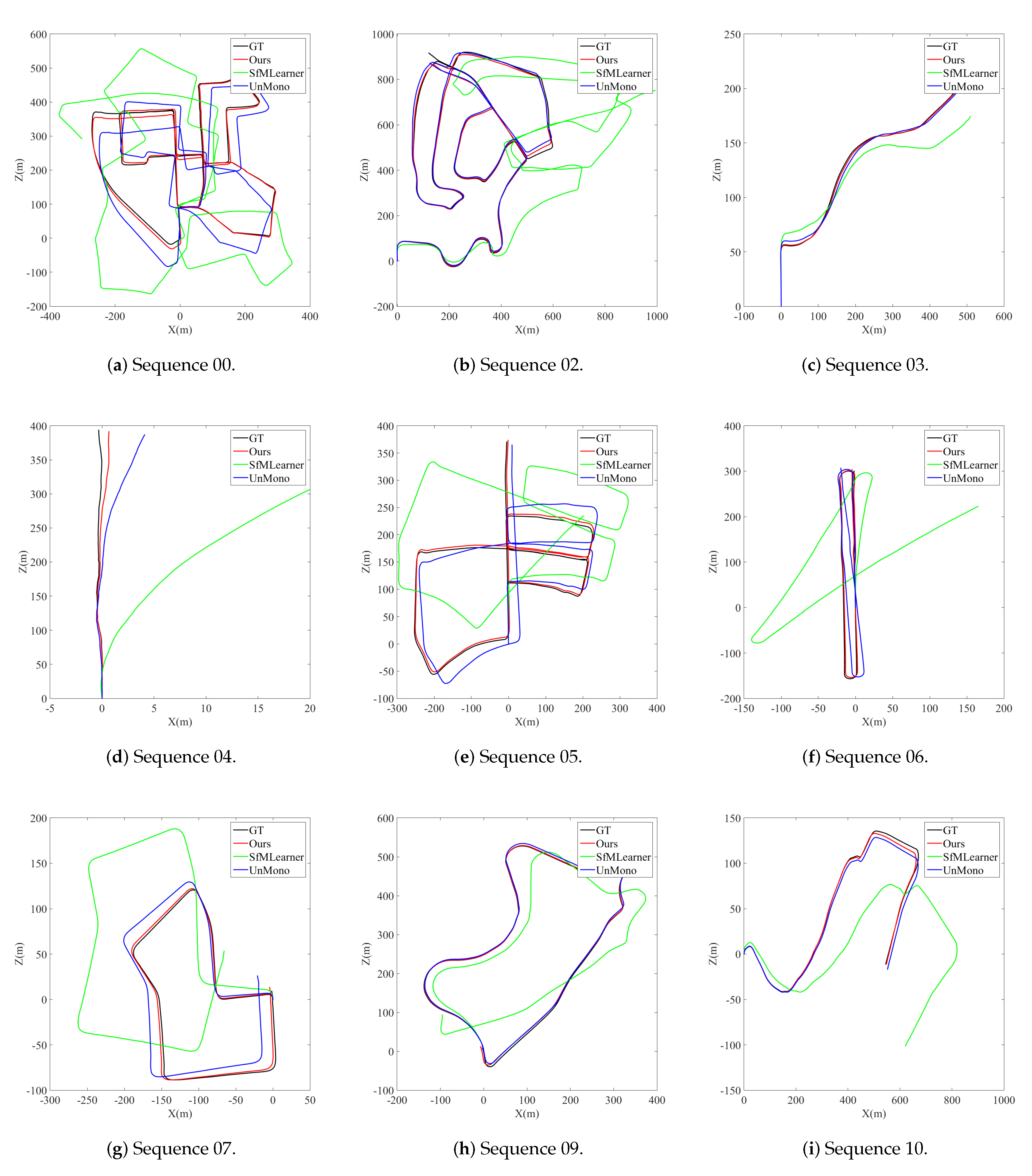
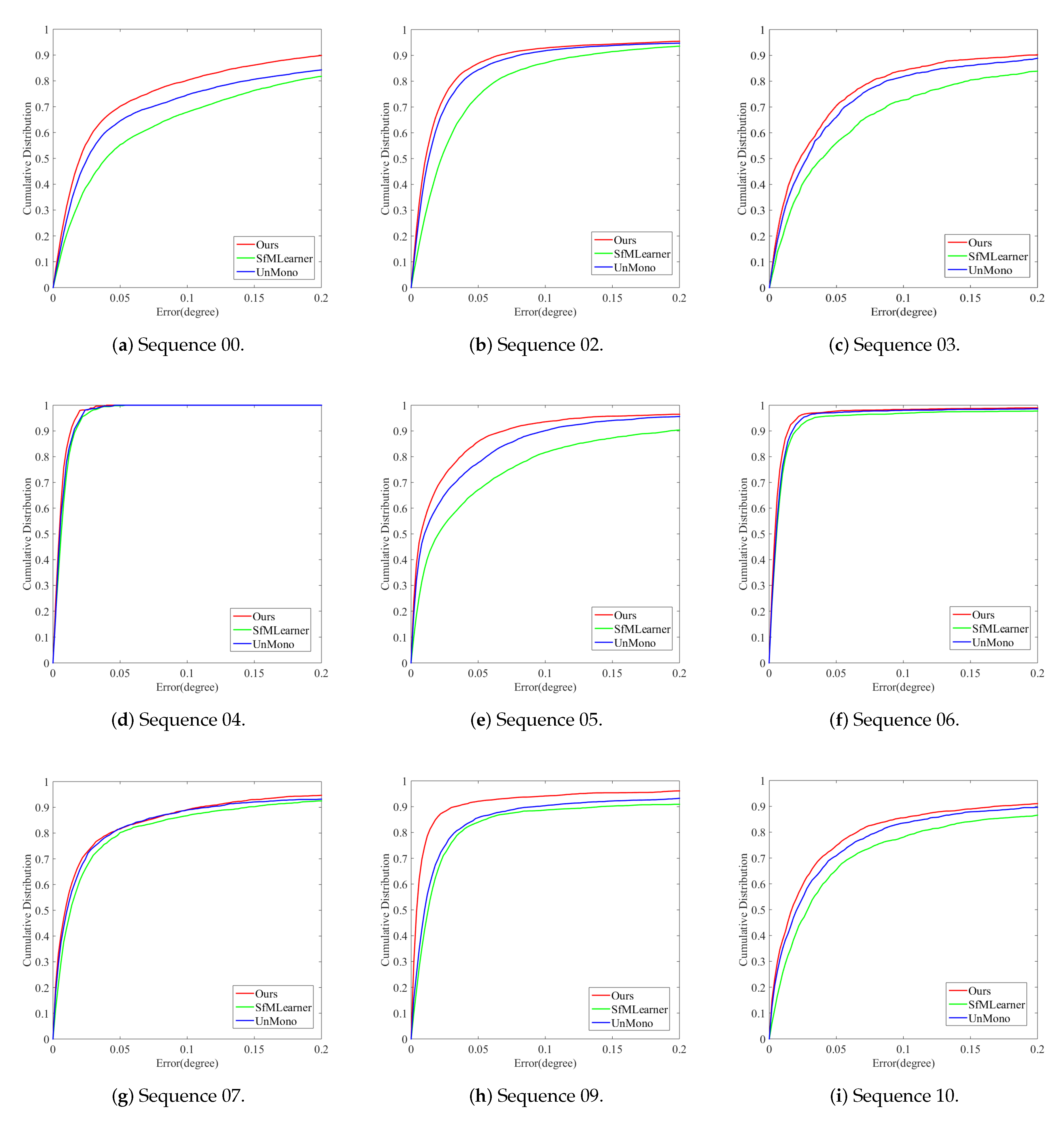
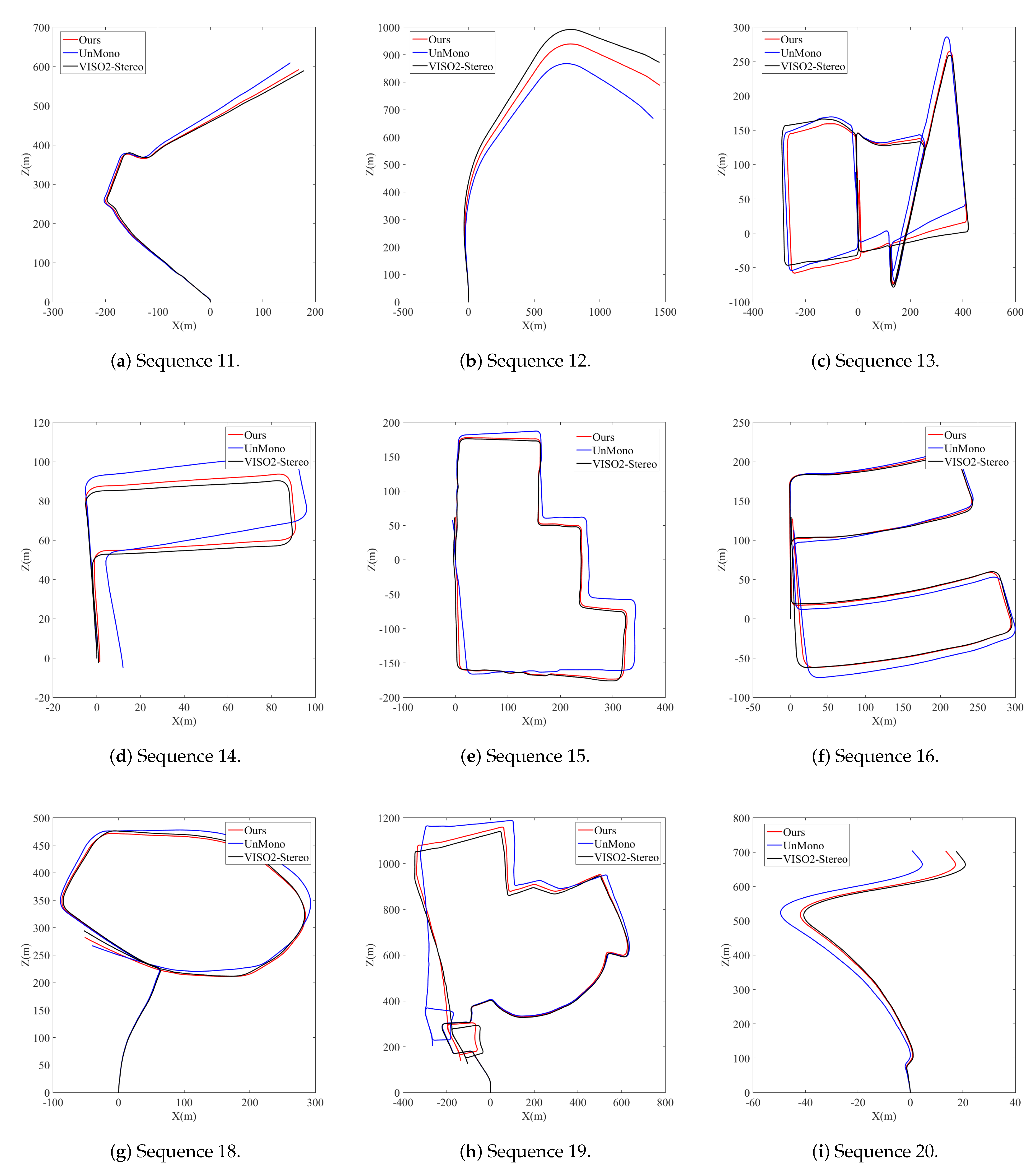
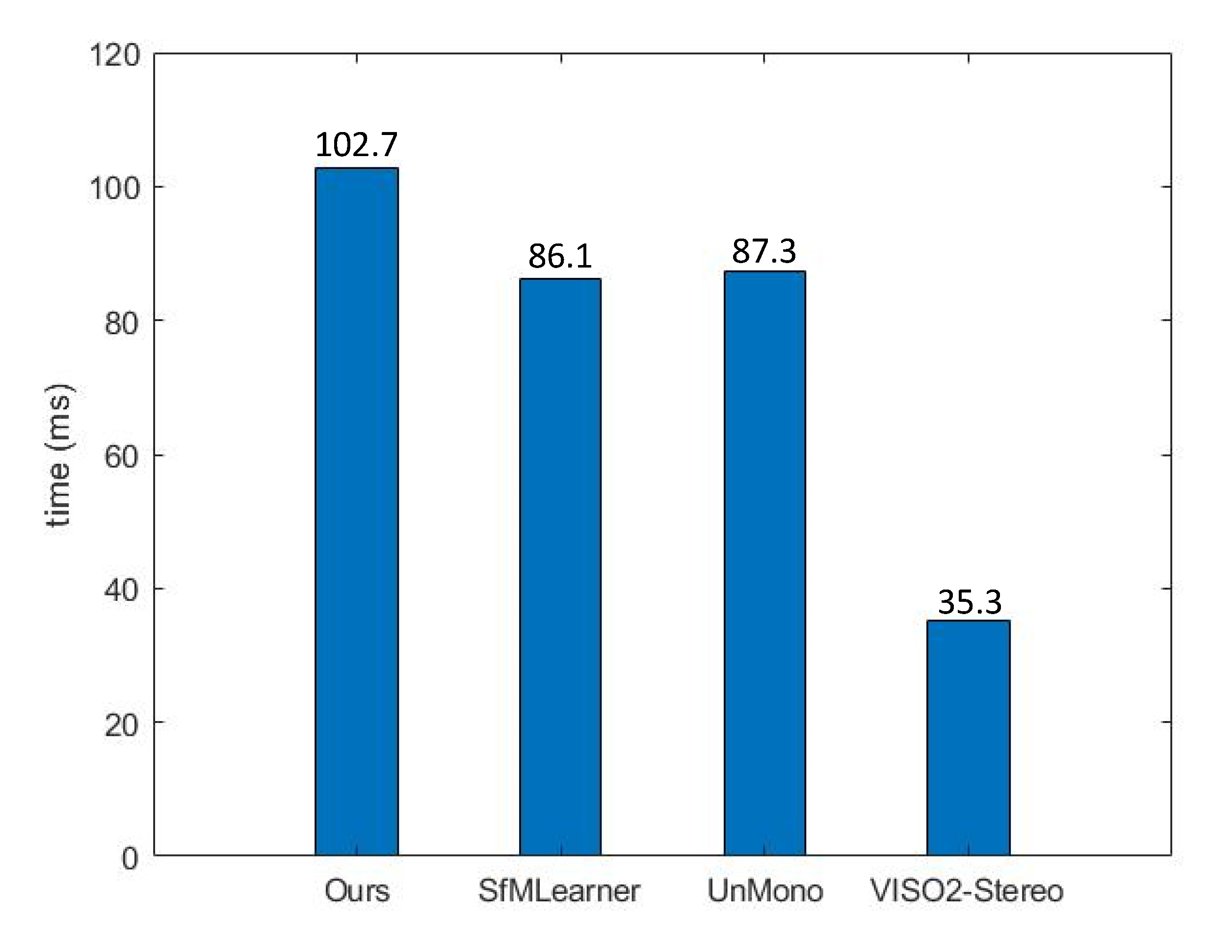
4.2. Performance Evaluation

The performance evaluation of the VO system was carried out on the KITTI Odometry dataset. Only sequence 00–10 in the dataset have ground truth, thus were used for quantitative analysis. Sequence 11–20 were used for additional qualitative analysis. We compared our system with SfMLearner, UnMono, and VISO2-Stereo. Our system, SfMLearner, UnMono are unsupervised deep learning-based. VISO2-Stereo is feature-based. SfMLearner poses were post-processed with ground truth depth information for scale recovery. SfMLearning and UnMono only used RGB images for inference, whereas we used RGB-D images. Since we were only evaluating odometry performance, loop-closure was not deployed. The same parameters were applied for all sequences in terms of each VO system.

The KITTY datasets are collected on a moving car. Since the vertical motion of the car is relatively small during driving, we ignore the vertical motion. In other words, in order to better show the effect in the figure, we omitted the z-axis. The trajectories of KITTI Odometry from Sequence 00 to 10 are presented in Figure 5. In Figure 5, the black curves represent the ground truth trajectory. The closer a trajectory is to the black curves, the better the system performance is. It is obvious that our system and UnMono performs better than SfMLearner in all sequences. The deviation mainly occurs when the car makes a turn. In other words, the accuracy of the predicted rotation matrix plays a vital role. Since no loop closure was applied, the noise accumulates and the deviation becomes obvious gradually. From Figure 5d,e,g, we can see the trajectories predicted from our system using additional depth information stay closer to the ground truth than UnMono which use only monocular images. The translation and rotation errors are reduced by more than half. Another point we should notice from Figure 5h,i is that although sequence 09 and 10 were not used for training, the system still performs well on these sequences, which indicates that the model is transferable on other similar scenes.

We further carried out a quantitative analysis of the transformation matrix estimation errors between neighboring frames. All errors were calculated based on two consecutive frames. Figure 6 depicts the cumulative histograms of translation error of our VO system, SfMLearner, and UnMono in terms of the aforementioned sequences. These figures show the distribution of translation errors in different ranges. When the translation errors are concentrated at a smaller value, the curves in the cumulative histogram approach the upper left corner, which indicates a better performance regarding translation estimation. In general, our VO system and UnMono perform better than SfMLearner. Furthermore, the maximum translation error of our system is relatively lower. In addition, our VO system is slightly better than UnMono, which is more obvious in Figure 6c–e. In Figure 6c, the translation errors of our VO system are all less than 0.2 m. The translation error of less than 0.2 m in UnMono accounts for 91%, and only 35% in SfMLearner.

Figure 7 depicts the cumulative histograms of rotation error of our VO system, SfMLearner, and UnMono. Similar to the evaluation of translation errors, the curves closer to the upper left corner indicate higher accuracy in terms of rotation estimation. We can see in all sequences, our VO system performs better than UnMono and SfMLearner, which is more obvious in Figure 7a,e,h. If we revisit the trajectories of these 3 sequences from Figure 5, we can tell they have more turns. In other words, our VO system outperforms UnMono and SfMLearner significantly in terms of scenes with more corners.

A detailed quantitative analysis is shown in

Table 2. Translational and rotational errors of our system, SfMLearner, UnMono and VISO2-Stereo. Our system, SfMLearner, UnMono are unsupervised deep learning based. VISO2-Stereo is feature based. SfMLearner poses were post-processed with ground truth depth information for scale recovery. Sequence 09 and 10 were not used for training.

	SfMLearner		UnMono		VISO2-Stereo		Ours
	Monocular		Monocular		Stereo		RGB-D
	Unsupervised		Unsupervised		Feature Based		Unsupervised
Seq.	${\mathit{t}}_{\mathit{rmse}}$	${\mathit{r}}_{\mathit{rmse}}\times 100$	${\mathit{t}}_{\mathit{rmse}}$	${\mathit{r}}_{\mathit{rmse}}\times 100$	${\mathit{t}}_{\mathit{rmse}}$	${\mathit{r}}_{\mathit{rmse}}\times 100$	${\mathit{t}}_{\mathit{rmse}}$	${\mathit{r}}_{\mathit{rmse}}\times 100$
00	45.89	6.23	5.14	2.13	1.86	0.58	2.97	1.53
02	57.59	4.09	4.88	2.26	2.01	0.40	1.83	1.71
03	13.08	3.79	6.03	1.83	3.21	0.73	3.21	1.15
04	10.86	5.13	2.15	0.89	2.12	0.24	0.94	0.57
05	16.76	4.06	3.84	1.29	1.53	0.53	2.31	1.03
06	23.53	4.80	4.64	1.21	1.48	0.30	1.25	0.80
07	17.52	5.38	3.80	1.71	1.85	0.78	1.47	1.31
08	24.02	3.06	2.95	1.58	1.92	0.55	1.91	1.20
09	22.27	3.62	5.59	2.57	1.99	0.53	1.86	0.50
10	14.36	3.98	4.76	2.95	1.17	0.43	1.15	1.17
mean	24.59	4.41	4.38	1.84	1.91	0.51	1.89	1.10

$t_{rmse}$ (%): average translational RMSE drift (%) on length of 100–800 m; $r_{rmse}$ (°/m): average rotational RMSE drift (°/m) on length of 100–800 m.

. Root Mean Square Error (RMSE) of translation and rotation are computed and listed. The values are averaged over all available errors on length 100, 200, …, 800 m. The smallest $t_{rmse}$ and $r_{rmse}\times 100$ in each sequence are shown in bold. Among the unsupervised deep learning systems, our system produces the lowest translation and rotation errors.

Trajectories of sequence 11–20 are shown in Figure 8. Since the ground truth of these sequences is not published, we have only conducted qualitative analysis and took VISO2-Stereo as a reference. The trajectory of VISO2-Stereo, our system, and UnMono are represented by black, red, and blue curves. From Figure 8d,h,i, we can tell our trajectories stay closer to VISO2-Stereo than UnMono, which again proves the importance of the additional depth information.

4.3. Discussion

Compared to our previous work, the main contribution of this paper is to incorporate an additional depth channel to the unsupervised VO system. The depth information is used for both network training and pose estimation. Experiments have shown that the proposed dual-channel network managed to reduce translation and rotation errors significantly during pose estimation. According to Table 2, the average RMSE of translation estimation ($t_{rmse}$) in terms of sequence 00–10 decreases from 4.38% to 1.89%, a drop of 56%, and the average RMSE of rotation ($r_{rmse}$) × 100 decreases from 1.84°/m to 1.10°/m, a drop of 40%.

However, we have observed the system suffered additional computational cost at the same time. In order to evaluate time complexity, we tested our VO system, UnMono, SfMLearner, and VISO2-Stereo on a DELL computer with an Nvidia GeForce GTX 980 GPU (Xiamen, China) with 4 GB memory. Figure 9 shows the time required for each camera pose estimation. It should be noticed that methods based on deep learning generally require more time than traditional feature-based methods. Our system, SfMLearner, and UnMono require a GPU for evaluation, whereas VISO2-Stereo relies on a single CPU and achieves a faster speed. After incorporating the depth channel, the time required for each camera pose estimation increased from 87.3 ms to 102.7 ms, an increase of 18%. In some cases, it is acceptable to sacrifice a small amount of computational power in order to effectively improve accuracy. However, computational efficiency is also an essential factor that should not be ignored. In the future, we will adjust our algorithm to further improve it.

On the other hand, compared to feature-based stereo VO system VISO2-Stereo, the translation error of our system is slightly smaller, but the rotation error is twice as high. This is because compared to translation, rotation is highly nonlinear, thus is more difficult to train. One possible solution is to increase the training dataset size and increase the ratio of rotational scenes.

5. Conclusions

This paper proposed a deep learning-based VO system, which can be viewed as a complement to traditional feature-based systems. RGB-D data is used for training and pose inference. The system adopts an unsupervised training framework. Experiments have shown that compared to monocular VO systems, the additional depth information can enhance the pose estimation accuracy and greatly reduce errors by half. Compared to other deep learning-based methods, our system directly yields predictions on an absolute scale without any scale post-processing. However, due to the additional depth information used for pose estimation, it is less computationally efficient than other VO systems.

In the future, we intend to take full advantage of the depth information and continue improving its robustness under challenging circumstances, especially when blurry monocular images and insufficient lighting conditions exist.

References

1. Nister, D.; Naroditsky, O.; Bergen, J. Visual odometry. In Proceedings of the 2004 IEEE Computer Society Conference on Computer Vision and Pattern Recognition, Washington, DC, USA, 27 June–2 July 2004. [Google Scholar]
2. Mukhopadhyay, S.C. Wearable Sensors for Human Activity Monitoring: A Review. IEEE Sens. J. 2015, 15, 1321–1330. [Google Scholar] [CrossRef]
3. Kendall, A.; Grimes, M.; Cipolla, R. PoseNet: A Convolutional Network for Real-Time 6-DOF Camera Relocalization. In Proceedings of the 2015 IEEE International Conference on Computer Vision (ICCV), Santiago, Chile, 7–13 December 2015; pp. 2938–2946. [Google Scholar]
4. Wang, S.; Clark, R.; Wen, H.; Trigoni, N. End-to-end, sequence-tosequence probabilistic visual odometry through deep neural networks. Int. J. Robot. Res. 2017, 37, 513–542. [Google Scholar] [CrossRef]
5. Kendall, A.; Cipolla, R. Modelling uncertainty in deep learning for camera relocalization. In Proceedings of the 2016 IEEE International Conference on Robotics and Automation (ICRA), Stockholm, Sweden, 16–21 May 2016; pp. 4762–4769. [Google Scholar]
6. Kendall, A.; Cipolla, R. Geometric Loss Functions for Camera Pose Regression with Deep Learning. In Proceedings of the 2017 IEEE Conference on Computer Vision and Pattern Recognition (CVPR), Honolulu, HI, USA, 2017; pp. 6555–6564. [Google Scholar]
7. Zhou, T.; Brown, M.; Snavely, N.; Lowe, D.G. Unsupervised Learning of Depth and Ego-Motion from Video. In Proceedings of the 2017 IEEE Conference on Computer Vision and Pattern Recognition (CVPR), Honolulu, HI, USA, 21–26 July 2017; pp. 6612–6619. [Google Scholar]
8. Li, R.; Wang, S.; Long, Z.; Gu, D. UnDeepVO: Monocular Visual Odometry Through Unsupervised Deep Learning. In Proceedings of the 2018 IEEE International Conference on Robotics and Automation (ICRA), Brisbane, Australia, 21–25 May 2018; pp. 7286–7291. [Google Scholar]
9. Mahjourian, R.; Wicke, M.; Angelova, A. Unsupervised Learning of Depth and Ego-Motion from Monocular Video Using 3D Geometric Constraints. In Proceedings of the 2018 IEEE/CVF Conference on Computer Vision and Pattern Recognition, Salt Lake City, UT, USA, 18–22 June 2018; pp. 5667–5675. [Google Scholar]
10. Liu, Q.; Li, R.; Hu, H.; Gu, D. Using Unsupervised Deep Learning Technique for Monocular Visual Odometry. IEEE Access 2019, 7, 18076–18088. [Google Scholar] [CrossRef]
11. Kitt, B.; Geiger, A.; Lategahn, H. Visual odometry based on stereo image sequences with RANSAC-based outlier rejection scheme. In Proceedings of the 2010 IEEE Intelligent Vehicles Symposium, San Diego, CA, USA, 21–24 June 2010; pp. 486–492. [Google Scholar]
12. Oskiper, T.; Zhu, Z.; Samarasekera, S.; Kumar, R. Visual Odometry System Using Multiple Stereo Cameras and Inertial Measurement Unit. In Proceedings of the 2007 IEEE Conference on Computer Vision and Pattern Recognition, Minneapolis, MN, USA, 18–23 June 2007; pp. 1–8. [Google Scholar]
13. Gamallo, C.; Mucientes, M.; Regueiro, C.V. Omnidirectional visual SLAM under severe occlusions. Robot. Auton. Syst. 2015, 65, 76–87. [Google Scholar] [CrossRef]
14. Wang, R.; Schwörer, M.; Cremers, D. Stereo DSO: Large-Scale Direct Sparse Visual Odometry with Stereo Cameras. In Proceedings of the 2017 IEEE International Conference on Computer Vision (ICCV), Venice, Italy, 22–29 October 2017; pp. 3923–3931. [Google Scholar]
15. Kerl, C.; Sturm, J.; Cremers, D. Dense visual SLAM for RGB-D cameras. In Proceedings of the 2013 IEEE/RSJ International Conference on Intelligent Robots and Systems, Tokyo, Japan, 3–7 November 2013; pp. 2100–2106. [Google Scholar]
16. Mur-Artal, R.; Tardós, J.D. ORB-SLAM2: An Open-Source SLAM System for Monocular, Stereo, and RGB-D Cameras. IEEE Trans. Robot. 2017, 33, 1255–1262. [Google Scholar] [CrossRef] [Green Version]
17. Whelan, T.; Kaess, M.; Johannsson, H.; Fallon, M.; Leonard, J.J.; McDonald, J. Real-time large-scale dense RGB-D SLAM with volumetric fusion. Int. J. Robot. Res. 2015, 34, 598–626. [Google Scholar] [CrossRef] [Green Version]
18. Geiger, A.; Lenz, P.; Stiller, C.; Urtasun, R. Vision meets robotics: The KITTI dataset. Int. J. Robot. Res. 2013, 32, 1231–1237. [Google Scholar] [CrossRef] [Green Version]
19. Engel, J.; Sturm, J.; Cremers, D. Semi-dense Visual Odometry for a Monocular Camera. In Proceedings of the 2013 IEEE International Conference on Computer Vision, Sydney, NSW, Australia, 1–8 December 2013; pp. 1449–1456. [Google Scholar]
20. Howard, A. Real-time stereo visual odometry for autonomous ground vehicles. In Proceedings of the 2008 IEEE/RSJ International Conference on Intelligent Robots and Systems, Nice, France, 22–26 September 2008; pp. 3946–3952. [Google Scholar]
21. Tardif, J.; Pavlidis, Y.; Daniilidis, K. Monocular visual odometry in urban environments using an omnidirectional camera. In Proceedings of the 2008 IEEE/RSJ International Conference on Intelligent Robots and Systems, Nice, France, 22–26 September 2008; pp. 2531–2538. [Google Scholar]
22. Khan, F.; Salahuddin, S.; Javidnia, H. Deep Learning-Based Monocular Depth Estimation Methods—A State-of-the-Art Review. Sensors 2020, 20, 2272. [Google Scholar] [CrossRef] [PubMed] [Green Version]
23. Kneip, L.; Chli, M.; Siegwart, R.Y. Robust real-time visual odometry with a single camera and an IMU. In Proceedings of the Proceedings of the British Machine Vision Conference, Dundee, UK, 29 August–2 September 2011. [Google Scholar]
24. Zhang, J.; Singh, S. Visual-lidar odometry and mapping: Low-drift, robust, and fast. In Proceedings of the 2015 IEEE International Conference on Robotics and Automation (ICRA), Seattle, WA, USA, 26–30 May 2015; pp. 2174–2181. [Google Scholar]
25. Debeunne, C.; Vivet, D. A Review of Visual-LiDAR Fusion based Simultaneous Localization and Mapping. Sensors 2020, 20, 2068. [Google Scholar] [CrossRef] [PubMed] [Green Version]
26. Ottonelli, S.; Spagnolo, P.; Mazzeo, P.L.; Leo, M. Improved video segmentation with color and depth using a stereo camera. In Proceedings of the 2013 IEEE International Conference on Industrial Technology (ICIT), Cape Town, South Africa, 25–28 February 2013; pp. 1134–1139. [Google Scholar] [CrossRef]
27. Carfagni, M.; Furferi, R.; Governi, L.; Servi, M.; Uccheddu, F.; Volpe, Y. On the Performance of the Intel SR300 Depth Camera: Metrological and Critical Characterization. IEEE Sens. J. 2017, 17, 4508–4519. [Google Scholar] [CrossRef] [Green Version]
28. Henry, P.; Krainin, M.; Herbst, E.; Ren, X.; Fox, D. RGB-D mapping: Using Kinect-style depth cameras for dense 3D modeling of indoor environments. Int. J. Robot. Res. 2012, 31, 647–663. [Google Scholar] [CrossRef] [Green Version]
29. Huang, A.S.; Bachrach, A.; Henry, P.; Krainin, M.; Maturana, D.; Fox, D.; Roy, N. Visual odometry and mapping for autonomous flight using an RGB-D camera. In Robotics Research; Springer: Berlin/Heidelberg, Germany, 2017; pp. 235–252. [Google Scholar]
30. Steinbrücker, F.; Sturm, J.; Cremers, D. Real-time visual odometry from dense RGB-D images. In Proceedings of the 2011 IEEE International Conference on Computer Vision Workshops (ICCV Workshops), Barcelona, Spain, 6–13 November 2011; pp. 719–722. [Google Scholar]
31. Sünderhauf, N.; Shirazi, S.; Dayoub, F.; Upcroft, B.; Milford, M. On the performance of ConvNet features for place recognition. In Proceedings of the 2015 IEEE/RSJ International Conference on Intelligent Robots and Systems (IROS), Hamburg, Germany, 28 September–3 October 2015; pp. 4297–4304. [Google Scholar]
32. Szegedy, C.; Liu, W.; Jia, Y.; Sermanet, P.; Reed, S.; Anguelov, D.; Erhan, D.; Vanhoucke, V.; Rabinovich, A. Going deeper with convolutions. In Proceedings of the 2015 IEEE Conference on Computer Vision and Pattern Recognition (CVPR), Boston, MA, USA, 7–12 June 2015; pp. 1–9. [Google Scholar]
33. Li, R.; Liu, Q.; Gui, J.; Gu, D.; Hu, H. Indoor Relocalization in Challenging Environments With Dual-Stream Convolutional Neural Networks. IEEE Trans. Autom. Sci. Eng. 2018, 15, 651–662. [Google Scholar] [CrossRef]
34. Wang, S.; Clark, R.; Wen, H.; Trigoni, N. DeepVO: Towards end-to-end visual odometry with deep Recurrent Convolutional Neural Networks. In Proceedings of the 2017 IEEE International Conference on Robotics and Automation (ICRA), Marina Bay Sands, Singapore, 29 May–3 June 2017; pp. 2043–2050. [Google Scholar]
35. Simonyan, K.; Zisserman, A. Very deep convolutional networks for large-scale image recognition. arXiv 2014, arXiv:1409.1556. [Google Scholar]
36. Kawakami, K. Supervised Sequence Labelling With Recurrent Neural Networks. Ph.D. Thesis, Technical University of Munich, München, Germany, 2008. [Google Scholar]
37. Jaderberg, M.; Simonyan, K.; Zisserman, A. Spatial transformer networks. In Advances in Neural Information Processing Systems; Neural Information Processing Systems Foundation, Inc.: London, UK, 2015; pp. 2017–2025. [Google Scholar]
38. Chen, Y.; Medioni, G. Object modelling by registration of multiple range images. Image Vis. Comput. 1992, 10, 145–155. [Google Scholar] [CrossRef]
39. Geiger, A.; Ziegler, J.; Stiller, C. StereoScan: Dense 3d reconstruction in real-time. In Proceedings of the 2011 IEEE Intelligent Vehicles Symposium (IV), Baden-Baden, Germany, 5–9 June 2011; pp. 963–968. [Google Scholar]
40. Kingma, D.P.; Ba, J. Adam: A method for stochastic optimization. arXiv 2014, arXiv:1412.6980. [Google Scholar]
Figure 1. Overview of the proposed visual odometry system.
Applsci 10 05426 g001
Figure 2. Architecture of the Convolutional Neural Network with input images.
Applsci 10 05426 g002
Figure 3. Architecture of the Recurrent Neural Network with output poses.
Applsci 10 05426 g003
Figure 4. Loss calculation for training.
Applsci 10 05426 g004
Figure 5. Sequence 00–10 trajectories.
Applsci 10 05426 g005
Figure 6. Sequence 00–10 Cumulative histogram of translation error.
Applsci 10 05426 g006
Figure 7. Sequence 00–10 Cumalative histogram of rotation error.
Applsci 10 05426 g007
Figure 8. Sequence 11–20 trajectories.
Applsci 10 05426 g008
Figure 9. Running time.
Applsci 10 05426 g009