Abstract
In this paper, methods are presented for designing a quadrotor attitude control system with disturbance rejection ability, wherein only one parameter needs to be tuned for each axis. The core difference between quadrotor platforms are extracted as critical gain parameters (CGPs). Reinforcement learning (RL) technology is introduced in order to automatically optimize the controlling law for quadrotors with different CGPs, and the CGPs are used to extend the RL state list. A deterministic policy gradient (DPG) algorithm that is based on an actor-critic structure in a model-free style is used as the learning algorithm. Mirror sampling and reward shaping methods are designed in order to eliminate the steady-state errors of the RL controller and accelerate the training process. Active disturbance rejection control (ADRC) is applied to reject unknown external disturbances. A set of extended state observers (ESOs) is designed to estimate the total disturbance to the roll and pitch axes. The covariance matrix adaptation evolution strategy (CMA-ES) algorithm is used to automatically tune the ESO parameters and improve the final performance. The complete controller is tested on an F550 quadrotor in both simulation and real flight environments. The quadrotor can hover and move around stably and accurately in the air, even with a severe disturbance.
1. Introduction
Quadrotor unmanned aerial vehicles (UAVs) have shown great potential for both civil and military applications, because of low cost, small volumes, simple structures, flexible operation, and vertical take-off and landing capability [1,2]. However, quadrotor UAVs present control challenges because of high-dimensional nonlinear dynamics, difficulties in measuring system parameters, and ever-changing noise and disturbances. Various control algorithms have been tested on quadrotor UAVs, among which the classic proportional-integral-derivative (PID) controller is the most widely used. For example, paper [3] presents a quadrotor UAV attitude control method to realize complex acrobatic UAV maneuvers using the double-ring PID algorithm and smith predictor. In paper [4], quadrotor attitude and position controller using rotation matrix based PID algorithm are designed. The linear quadratic regulator (LQR) algorithm has also being used in quadrotor UAVs with some success [5]. Researchers compared the performance of a Qball-X4 quadrotor with PID controller and LQR controller, and the tracking trajectory with LQR controller is more smooth and it has less disturbance [6]. LQR algorithm can also be applied on a morphing quadrotor and achieve a success [7]. Nonlinear control algorithms, such as back-stepping (BS), sliding mode control, and H-infinity control, have been applied to quadrotors. Researchers propose an approach of the backstepping control running parallel with a sliding mode observer for a quadrotor UAV [8,9]. Paper [10] presents quadrotor altitude control with sliding mode control and paper [11] designed attitude and position control using sliding mode control. H-infinity control is another optimal control algorithm that provides a robust stable closed-loop system with high performance tracking and disturbance rejection. Paper [12] present H-infinity style quadrotor attitude controller, where the system transfer function is identified based on input and output experimental data. In paper [13], a H-infinity observer is designed to compensate the effect of actuator failures, sensor failures, and external disturbances. However, these algorithms rely heavily on model accuracy, which severely affects application to real quadrotor platforms.
The active disturbance rejection controller (ADRC) technique is based on the traditional PID: a tracking differentiator (TD) is set to arrange the transition process and extract the differential signals, and an extended state observer (ESO) is used to estimate the state of the control object and the unknown disturbances. A nonlinear state error feedback (NLSEF) is formed by a nonlinear combination of the results from the TD and the ESO, including the compensation for external disturbances if needed [14]. Both external disturbances and model errors can be estimated while using ESOs. The critical gain parameter (CGP) is the gain in the input channel that characterizes the proportional relation between the input signal and the derivative of the process output of a specific order [15]. In this paper, the CGP is the proportional relation between the control signal and the angular accelerations of three axes. Studies have shown that the ADRC can be used to stably control a quadrotor in the presence of external disturbances [16,17,18].
Acceptable control performance have been demonstrated for the control systems proposed by previous researchers. However, model-based control algorithms, such as LQR and BS, heavily rely on model accuracy, which hinders their application to real quadrotor platforms. It is difficult to tune the parameters of model-free algorithms, such as PID and ADRC. When considering the traditional double-ring PID algorithm as an example, typically three or more parameters must be tuned for each axis, and the tuning process can be time consuming and dangerous. For quadrotor systems, automatic tuning algorithms, such as the genetic algorithm (GA) and particle swarm optimization (PSO), can be tested in simulation environments, but it is unsafe to automatically explore control parameters during real flight experiments. In this paper, we present an Reinforcement learning (RL) method to achieve single-parameter-tuned attitude control. Thus, the difficulty of multi-parameter tuning in PID-based algorithms is reduced.
RL is an automated self-optimization method that allows for agents to explore the environment and collect experience to improve performance. Agents output actions and receive rewards during the exploration process, and the controller, referred to as the policy in this frame, constantly optimizes itself based on experience to obtain higher rewards. The process can present optimal or at least locally optimal controllers, which is sufficient for solving a complex control problem in many cases. RL algorithms have been introduced into the UAV control area with remarkable achievements [19,20]. Andrew Ng et al. used the RL method to design a flight controller for the Stanford autonomous helicopter [21]. A data-driven approach was used to determine the system model, which is, flight data were collected and fitted using a locally weighted linear regression algorithm. These approaches are effective for some specific experimental platforms, but cannot be directly transferred to other types of platforms, and measuring of system parameters or identifying system models can be difficult and expensive. An alternative approach is to train a policy that is sufficiently robust in order to neglect model errors as well as potential disturbances. For example, computer-aided design (CAD) has been used to obtain the parameters of a quadrupedal robot in [22], and noise and disturbances can be added to either the system models or sensor data during the training process. We tested this method on a quadrotor in our previous study, and the trained policy was effective for platforms with different system parameters in a simulation environment. However, the performance for each platform may be less ideal than a full tuned PID controller.
In this paper, a new method is presented in order to achieve simple tuning control with RL: that is, we extract the core difference of platforms as critical system parameters that are then included in the state list during the RL training process. This method can be used to apply the trained controller to different platforms, and excellent performance can be achieved with simple parameter tuning. The critical system parameters for quadrotor UAV systems include the moment of inertia, the lift coefficient, the torque coefficient, etc. We extract these parameters as CGPs for the three axes, which is a key step in the ADRC algorithm. This method can be used to apply the RL controller to different quadrotors, where only one parameter CGP needs to be tuned for each axis.
In many previous studies, RL controllers have exhibited excellent performance, including a fast convergence rate with hardly any overshoot, but they have failed to eliminate steady-state errors. These errors remain distinct, irrespective of how the hyperparameters are set and the types of exploration strategies applied [23]. In [23], integral compensators are added to the quadrotor system to eliminate steady-state errors, but our simulation experimental results show that this method may reduce the final performance. Thus, we develop novel methods, i.e., reward function shaping and mirror sampling, to solve the steady-state error problem that is incurred using RL algorithms. Ideal results with nearly no steady-state error are obtained, and the training process is considerably accelerated.
External disturbances to a quadrotor are compensated for by designing a set of ESOs to estimate the total disturbance of the roll and pitch axes, where the total controller output is the combination of the RL controller output and the ESO feedback. However, it is difficult to tune the parameters of an ESO. Inappropriate ESO parameters cause high frequency vibration problems in both simulation and real flight experiments, which may reduce the control quality. In this paper, an efficient and powerful metaheuristic algorithm, which is referred to as the covariance matrix adaptation evolution strategy (CMA-ES), is introduced to automatically adjust the ESO parameters. The CMA-ES is a type of random numerical derivative-free optimization algorithm with a superior efficiency and success rate to GA and PSO [24].
In this paper, the CMA-ES algorithm is designed to reduce the error between the ESO output and the real disturbance. Disturbance measurement is challenging. We meet this challenge by designing a specialized test: the quadrotor is placed on the ground in the absence of an external disturbance, and control signals are sent to the controller; however, the motors are not actuated and they remain still during the test. In this situation, from the perspective of the controller, a disturbance compensates for the control signals to keep the quadrotor still, such that the value of the disturbance is simply the negative of the current control signals multiplied by the CGP. This test prevents problems, such as safety risks, computational costs, and battery capacity limitation, and we can run the CMA-ES algorithm directly on a real quadrotor.
In this paper, the quadrotor attitude control is divided into three second-order linear systems with different CGPs and disturbances. We lock the pitch and yaw axis of a quadrotor as a standard second-order linear rotation system rather than using a full quadrotor during RL training process. Our RL algorithm is based on the deterministic policy gradient (DPG) algorithm with two actor neural networks (NNs) and two critic NNs. Mirror sampling and reward shaping methods are introduced to the training process to eliminate the steady-state errors of the RL controller and accelerate the training process. The CGPs of the quadrotor platforms are recognized while using TDs, and the CGPs can also be manually tuned in a real flight environment. The CMA-ES algorithm is used to automatically conduct ESO parameter tuning in both a simulation environment and a real quadrotor. The controllers are well-trained and tuned and they are also tested in a quadrotor simulation system. Finally, the controller is applied to a real F550 quadrotor. The program is run on a Raspberry Pi microcomputer, which is sufficiently fast to run the NNs in real time. The quadrotor can hover and move around stably and accurately in the air even under severe disturbances.
The main contributions of this paper are summarized below:
- (1)
- In this paper, RL is used to develop a single-parameter-tuned quadrotor attitude control system that exhibits excellent performance in both simulation and real flight experiments. This method offers the considerable advantage of requiring one parameter CGP to be tuned for each axis. Critical system parameters are used to extend the RL state list, making the same RL network suitable for platforms with different system parameters, which represents an advance in RL theory.
- (2)
- The introduction of reward function shaping and mirror sampling eliminate the steady-state errors incurred using RL control systems and considerably accelerate the training process.
- (3)
- ADRC methods are used to eliminate external disturbances to the quadrotor attitude control system in real time. A practical method is developed to automatically tune the ESO parameters using CMA-ES for a real quadrotor.
The remainder of this paper is organized, as follows. In Section 2, a nonlinear quadrotor system model is established, and identification methods are introduced. A RL control algorithm and a CMA-ES parameter tuning algorithm are developed in Section 3. In Section 4, the training details and results are presented, and the simulation experiments are discussed. Section 5 presents the ESO tuning details for a real quadrotor platform and the performance of real flight experiments using the RL controller. Section 6 concludes the paper.
2. System Model and Identification
In this paper, an “X” type F550 quadrotor is used and tested, and its structure and frame are presented in Figure 1. The attitude of the quadrotor represents the angular error between the body frame and the earth frame.In Figure 1, represent the roll, pitch, and yaw angles, respectively, while to represent angular velocities of four rotors.
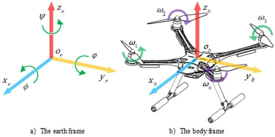
Figure 1.
Coordinate definition.
The rotation of a quadrotor can only be controlled by changing the lift force and torque of the four rotors. The rigid-body dynamic model of the quadrotor in this paper can be derived from the Newton–Euler equation:
where are angular velocities of the quadrotor. are the moment of inertia in three axes. are torque generated by rotors. are disturbance torque in three axes, including aerodynamic drag, side wind, center of gravity shift, physical impact, and model error. The torque of three axes are determined by the angular velocities of four rotors:
where is the lift coefficient and is the torque coefficient of the rotors. d denotes the length of arm of the quadrotor. and are intermediate variables. are scale constants, to are theangular velocities of the four rotors in Figure 1. are the results of attitude controller. The relationships between and can be modeled as a first order system:
where and denote the current angular velocity and the desired angular velocity, is the dynamic response constant of the motor-rotor system.
The accuracy of these parameters is critical. The mass and length can be measured directly, but the measurement of other parameters is difficult. Mechanical parameters, such as moment of inertia, are directly calculated in the Solidworks software package in this paper. The physical parameters of motors and propellers are measured with a motor test beach. The remaining of unknown parameters, including and , can be found in a quadrotor data base online: https://flyeval.com/[25].
A simulation environment program in which the quadrotors’ states can be updated with the control signals of motors is built with the system model and parameters. The attitude of quadrotors is represented with unit quaternions and updated with the traditional Runge-Kuta method, as shown in Equation (5).
where is a group of unit quaternion to describe the rotation between the quadrotor body and earth frame. The quaternion in this paper is a unit quaternion:
where is the total rotation (the combination of roll, pitch, and yaw rotation) and are projections of in the axes. We limit between and , so is positive all the time. When is not too large, the attitude angle of roll, pitch, and yaw can be simplified as , respectively.
3. Quadrotor Attitude Control System Design
The attitude controller receives the desired attitude , the current attitude , and the current angular velocities and then outputs the control values of each axis according to the states. The CGPs of each axis are estimated or tuned manually. The disturbance of roll and pitch axes is estimated by the ESOs. Finally, the control distributor transfers and to the ( and, in return, sends the attenuated control values to the ESOs because the actual control value of each axis may be attenuated by the control distributor if is too large or too small. Figure 2 presents the control diagram.
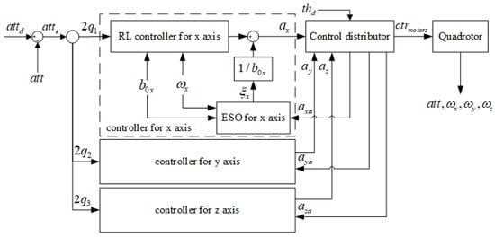
Figure 2.
The quadrotor attitude control system diagram.
The typical ADRC comprises three major components: the nonlinear tracking differentiator (TD), extended state observer (ESO), and state error feedback (SEF) [14]. In the traditional ADRC, the transient process is set to avoid a sharp deviation between reference signals, and the process is realized through the TD. In this paper, the transient process is automatically employed by the RL method. The CGP is the estimation of the system response capability, and the accuracy of CGP is critical to the performance of both the ESO and SEF. In previous studies, CGPs were the manually adjusted parameters. We propose a method to estimate the CGP value for each quadrotor platform with a TD. With ESOs and CGPs, the RL controller is able to control different quadrotors with the same actor network. In order to optimize the final performance, the CMA-ES algorithm is presented to tune the parameters of ESOs, and succeeded eliminating the high frequency vibration problem.
3.1. First-Order ESO and SEF for Quadrotor Attitude Control
In a quadrotor attitude control system, taking the x axis as an example, the system can be written as:
where is the estimation of the CGP and is the estimation of the total disturbance. The ADRC algorithm takes the nonlinearities, uncertainties, and external disturbances as the total disturbance. The total disturbance can be observed by the ESO in real time with the quadrotor state input, the control output, and an estimation of CGP. The quadrotor control system receives angular velocity data directly from the gyroscope sensors, so the form of the ESO for the quadrotor attitude control system in a single axis is a first-order ESO (Algorithm 1):
| Algorithm 1 Extended state observer for quadrotor attitude control. |
y: angular velocity data from sensors : angular velocity output : disturbance output h: time step : critical gain parameter u: control output : intermediate variables : adjustable parameters : a non-linear function [14]
|
Using the ESOs, the disturbance of three axes are estimated, and the disturbance feedback should be added to the controller output:
where a is the final control value and is the output of the controller.
In this paper, only roll and pitch ESOs are designed, because the yaw axis is hardly affected by the external disturbances in our outdoor flight experience. In severe flight situations, such as propeller breakage and load swinging, the control system should focus on maintaining the balance of the roll and pitch axes, and the performance of the yaw axis may not be so important.
3.2. Estimation of the CGPs
In this paper, the CGP is the proportional relation between the control signal and the angular accelerations in three axes . The accuracy of the CGPs is critical to both the RL controller and ESO feedback. The CGPs of the F550 quadrotor can be simply calculated with Equation (8), but the measurement of different quadrotors or platforms can be difficult and expensive and, thus, a method to estimate the CPGs is presented in this section.
As Equation (7) shows, the CGP can be calculated given the state of a quadrotor, including angular acceleration, control value, and disturbance. When considering the ill-conditioned equation problem and noise of sensors, the system should obtain enough excitation during the estimation process, but too much excitation may cause a quadrotor crash. To precisely estimate angular acceleration data, a TD is designed to calculate the differential of angular velocity data in Algorithm 2:
| Algorithm 2 Tracking differentiators for angular velocity data. |
: angular velocity data from sensors : angular velocity output : angular acceleration output : a non-linear function [14] : intermediate variables h: time step : adjustable parameters, usually two or three times h
|
The estimation process starts when the quadrotor hovers stably above an open and wide ground. The controller produces an excitation for s on a single axis, and then the CGP in this axis can be calculated with these flight data.
3.3. Single-Parameter-Tuned Attitude Control Method
The RL method is a frame with these key factors: the agent, environment, state , policy , action , reward , and state-action value . During the training process, the agent takes action according to state and policy in the environment, and obtains a reward in return. Value is the sum of the expected future rewards:
where discount factor is introduced to prevent the infinite sum of future rewards. However, the future reward is unknown, so we assume that an optimal policy can maximize :
where A is the action space. During the training process, we use the current policy instead, and this process can make the performance of gradually close to .
With the ADRC methods, the quadrotor attitude control is divided into three second-order linear systems with different CGPs and disturbances, so we lock the pitch and yaw axis of a quadrotor as a standard second order linear rotation system rather than a full quadrotor. The agent is similar to an inverted pendulum, which explores the rotation space while discovering the optimal policy and tracking the desired roll angle. Accordingly, the system state variables in training process are represented as: is the attitude angle, is the angular velocity, is the CGP of this axis and is the control output. Actuator delay is also considered as a first order system in Equation (4). During the training process, no disturbance is added in the simulation.
3.3.1. Network Structures
The RL controller in this paper is based on the actor-critic scheme [26], in which the critic network judges the value of a state-action-pair, and the actor network outputs the control values according to the states input. The state in the attitude control process consists of the error between the desired attitude and the current attitude, along with the current angular velocity. The CGP is added to the state in this paper, so the state list is written as: . The action list is expressed as , where is the control value in the controlled axis.
We have two critic networks with the same structure: target critic network and online critic network [26]. The critic networks are fully connected networks (FCNs), with a hidden layer of 32 nodes and ReLU activation function. All of the experience is used to train the online critic network to fully observe the system and compute the value . After that, we define the cost function as a squared error function and lower the cost using the Adam optimizer. The target critic network is soft updated with an online critic network.
The online actor network and target actor network are also FCNs with a 32-node ReLU hidden layer. The tanh activation function is set in the output layer to limit the output between −1 and 1. The state lists are sent directly to the actor network and action lists are computed. The gradients of the online actor network are computed with sampled policy gradients directly and then update the weights with the Adam optimizer [27]. The target actor network is soft updated [26] with the online actor network as well. Figure 3 presents the structures of actor networks and critic networks.
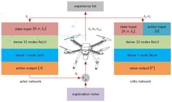
Figure 3.
Network structures.
3.3.2. Reward Function Shaping and Mirror Sampling Methods
Reward function shaping and mirror sampling methods are presented in order to eliminate the steady-state error problem of RL algorithms in this section.
Traditionally, the reward functions are squared error functions such as , where and are positive parameters. However, these squared error reward functions lead to slow convergence rates and severe steady-state error problems in our former experiments. From the perspective of this paper, the state with a low angle error or low angular velocity should be rewarded positively rather than be punished with less penalty. This paper presents a simple but powerful piecewise function to meet this demand:
where x is the angle error or angular velocity to be rewarded, is the upper level of x, and is the boundary line. If , then x should be rewarded positively. With , the reward function is designed as:
where and are positive parameters to be tuned.
Because the quadrotor attitude control system is a symmetrical system, whenever a list of experience is explored, the mirror sample experience is also correct. Moreover, the zero state-action point is an obvious result, but may never be explored in the training process, which is an important reason for the steady-state error problem. These samples should be considered to accelerate the training process and eliminate steady-state errors.
3.3.3. Training Algorithm
The training algorithm in this paper is the DPG algorithm [26], and we add some Gaussian noise to the action as the exploration strategy. Algorithm 3 lists the whole algorithm.
| Algorithm 3 Training algorithm with mirror sampling. |
: max number of episodes : max number of steps in an episode : max number of samples : reward function in Equation (13) : soft update rate
|
3.4. ESO Parameter Tuning with CMA-ES Algorithm
Although there are some rules about parameter tuning in ESO, it is still repetitive work, even for designers with considerable experience. The parameters to tune are a list of in Algorithm 1 for the roll and pitch axes. In this section, only the ESO in the roll axis is optimized.
In the simulation environment, the disturbance can be directly obtained, so we optimize the process during flight, and the controller is the actor network trained in Section 3.3, along with the disturbance feedback that is calculated by the ESO. A task is designed to test and quantify the performance of the ESO. The system starts on the zero point state, and the controller tries to hold the system on the zero point state for a period of time, with the same time-varying square wave disturbance added to the system in each test. The costs in each task are computed with the error of ESO output and disturbance in every time step during the task.
In the real quadrotor platform, we designed a specific test: the quadrotor is placed on the ground with no external disturbance, and control signal is sent to the controller; but, the motors are not actuated and remain still during the test. It is worth noting that the control signal here is not computed by the controller in Section 3.3; we set as a square wave. In this situation, from the perspective of the controller, a disturbance compensates for the control signals to keep the quadrotor still, so the value of disturbance is just the negative of current control signal multiplied by the CGP . Using this test, we avoid problems, such as safety risks, computational costs, and battery capacity limitation, etc. The task for real quadrotor optimization is that the system starts on the zero point state and holds still for a period of time, and the same time-varying control signal is added to the system in each test. The costs in each task are also computed with the error of and in every time step during the task.
We present ESO parameter tuning with the CMA-ES algorithm in this section. The CMA-ES algorithm is a stochastic or randomized method for real-parameter (continuous domain) optimization of nonlinear, nonconvex functions. The CMA-ES algorithm consists of five parts: sampling, calculating costs, updating the mean value, adapting the covariance matrix, and step-size control [24].
3.4.1. Sampling
In the CMA-ES, a population of new search points (individuals, offspring), is generated by sampling a multivariate normal distribution :
The parameter is the mean value, is the step-size (scale value), is a search point sampled from multivariate normal distribution , and is sampled from . results from an eigendecomposition of the covariance matrix . The columns of are an orthonormal basis of the eigenvectors. The diagonal elements of the diagonal matrix are the square roots of the corresponding positive eigenvalues. In fact, CMA-ES controls the search directions with the matrix , and controls the search range with and .
3.4.2. Calculating Costs
It is critical to lower the error between the real disturbance and the estimation output of the ESO in order to eliminate the high frequency vibration problem. The tasks in the simulation and real quadrotor platform presented above are tested for all search points. For every search point , the cost in every time step is computed with , and the total cost is the sum of all costs in every time step.
3.4.3. Updating the Mean Value
The mean value of next generation is updated based on the costs above. We sort these costs and only the first samples are recorded: . A list of weights is designed in the beginning of the algorithm, and is calculated with these weights:
3.4.4. Adapting the Covariance Matrix
The covariance matrix determines the search directions. Two methods to update the : rank-1 update and rank- update are presented in this section. The rank-1 update means that we should search new points in the direction of the new mean value:
where is the evolution path, c is the learning rate of the evolution path update, and . The rank- update means we should search new points in the direction of the search points with low costs. As a result, the covariance matrix updates with the equation below:
where and are the learning rates for the rank-1 update and the rank- update.
3.4.5. Step-Size Control
This section presents a simple method to control the step size . We scale according to the mean value :
where is the max step-size, and is the max cost we set.
Algorithm 4 lists the total algorithm:
| Algorithm 4 Covariance matrix adaptation evolution strategy (CMA-ES) algorithm for extended state observer (ESO) parameter tuning. |
: max number of generations
|
4. Training and Testing in the Simulation
4.1. Training Environment
A simulation environment is developed to train and test the UAV controller. The program is coded with Python 3.8 and TensorFlow 1.14. Quadrotors with different physical parameters can be created, and their performance can be tested in the environment. The training and testing processes are conducted on a laptop computer with an NVIDIA GTX1060 graphics processing unit (GPU) and i7-7700HQ central processing unit (CPU).
4.2. Performance in the Simulation and Details
4.2.1. Quadrotor Details
The quadrotor UAV used in this paper is an “X” type F550 quadrotor, equipped with TMOTOR 2213 brushless motors, TMOTOR 9545 propellers, SKYWALKER 30A Electronic Speed Controls (ESCs) and an ACE 5300mAh 30C 3S Li-polymer battery. The adjustable timing of the ESC is set to a medium level to achieve better performance. With these parameters, the CGPs of the three axes can be calculated. Table 1 lists the system parameters.

Table 1.
Physical parameters of the quadrotor.
We estimated other types of quadrotors such as an F250 traversing machine and a 10 kg grade agricultural plant protection quadrotor. The CGPs of the x and y axes are between 50 and 200, and the CGPs of the z axes are between 3 and 10. The range of CGPs is limited between 1 and 200 in this paper as a result.
4.2.2. Performance of the RL Controller and Training Details
Taking the roll and pitch attitude control as an example, the step response and sine function tracking performance is shown in Figure 4:
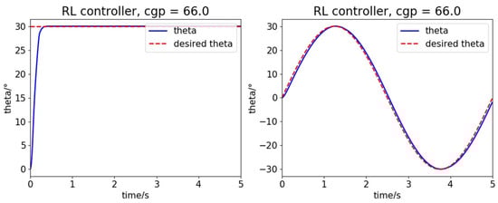
Figure 4.
Step response and sine function tracking performance.
The performance is excellent with a high convergence rate and nearly no overshoot and steady-state error. In theory, the RL controller grows close to the global optimal controller with sufficient proper training, which performs better than any other traditional controller.
The controller in this paper has great robustness for different types of quadrotors with different CGPs. We test the performance of quadrotors with different CGPs (cgp = 6.0, 66.0, 100.0, 180.0) in Figure 5. The quadrotors start with random states (attitude angles and angular velocities) and recover to zero points with the RL controller, and this process is tested for 100 times. The network here is fully trained for 1000 episodes. All of the quadrotors perform excellently and we can conclude that the rate of convergence improves with larger CGP value.
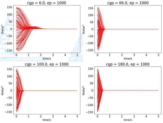
Figure 5.
The robustness of quadrotors with different CGPs.
The training process improves the performance gradually, and the performance of controllers in different episodes (ep = 0, 100, 200, 1000, respectively) is tested in Figure 6. The same quadrotor (cgp = 66.0) is tested here to recover from random initial states 100 times. The controller functions better during the training process as a result.
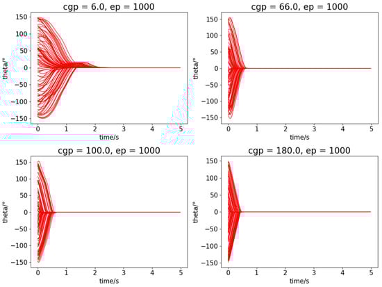
Figure 6.
The performance of the controller in different episodes.
The reward shaping and mirror sampling method greatly accelerates the training process and improves the control quality. In Figure 7, the reward function of this RL controller is a traditional squared error function , and the controller is fully trained with 1000 episodes. The performance of this RL controller without the reward shaping and mirror sampling method is not so good in the step response task and sine function tracking task as compared to the RL controller in Figure 4; the response rates are too low and the steady-state errors are obvious.
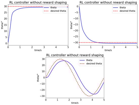
Figure 7.
The performance of the RL controller without the reward shaping and mirror sampling method.
The total training process took approximately 12 min. The hyperparameters of the training process are listed in Table 2.
Table 2.
Reinforcement learning (RL) training hyper parameters.
4.2.3. CMA-ES Training Detail in the Simulation Environment
In this section, square wave disturbances are added to the system. The system with no ESO feedback cannot overcome the effect of these disturbances, as the first picture in Figure 8 shows. CMA-ES searches for better to reduce the cost, and the performance of the total controller also improves. In Figure 8, the CMA-ES algorithm improves the performance gradually as the generation grows ( respectively) and finally converges to .
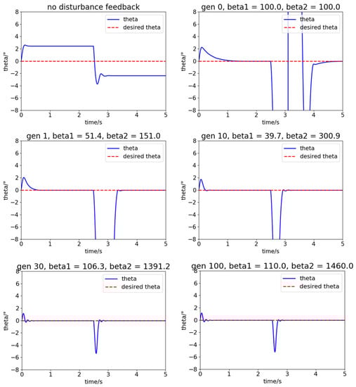
Figure 8.
The performance of the controller with ESO in different episode.
The total training process took approximately 16 min. The hyperparameters are listed in Table 3.
Table 3.
CMA-ES training hyper parameters in simulation.
4.2.4. Performance of the Full Controller
The quadrotor attitude controller combined RL with ADRC in this paper has excellent performance, including a fast convergence rate, nearly no overshoot and steady-state error, a high robustness for different platforms, and a strong disturbance rejection ability. In Figure 9, the quadrotors with different CGPs perform well in the step response test with the same external disturbance. The disturbance is a square wave, but the final performance compensates for the disturbance completely in a timely manner. The overshoot angle and final steady-state errors are less than 0.001 degrees, which can be ignored. The 30 degrees step-response take less than 0.35 s, which show great convergence rate. In conclusion, the performance in Figure 9 meet our demand for a quadrotor attitude control system. The performance of these quadrotors also indicate that the convergence rate and the disturbance rejection ability of a quadrotor can be improved with a larger CGP value.
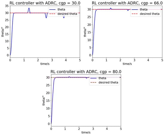
Figure 9.
The performance of the controller in this paper with severe external disturbances.
We designed a traditional PID controller for comparison. The PID parameters are also optimized with the CMA-ES algorithm, and this controller can be considered as a near-optimal PID controller. In Figure 10, the PID controller is not as good as that of our RL controller. The control quality of the PID controllers is limited due to the conflict between rapidity and stability, and the RL controller can solve the problem with enough exploration during training. When compared to the traditional PID controller, the RL controller in this paper only has one parameter to tune, which is a great advantage.
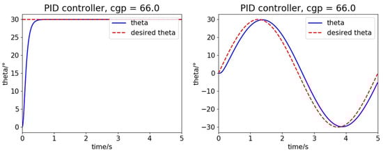
Figure 10.
The performance of automatically tuned traditional proportional-integral-derivative (PID) controller without outer disturbance.
Notably, parameter I in the PID controller converges to 0 during the CMA-ES optimization process. However, the integral controller can also compensate for disturbance over time. We manually set parameter I as a small value in the next experiment. As Figure 11 shows, if the external disturbances are added to the system, then the PID controller is unable to compensate for these errors in a timely manner, and the compensation efficiency of integral controllers is not sufficient.
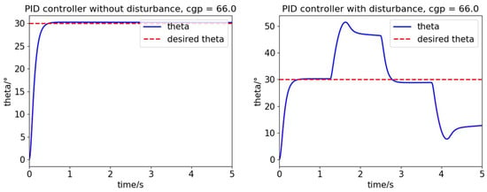
Figure 11.
The performance of the traditional PID controller with external disturbances.
In conclusion, the controller in this paper has shown greater advantages than the traditional PID controller in control performance, robustness for system models, and external disturbance.
5. Experiments
The flight controller is based on a Raspberry Pi 3B microcomputer whose CPU has four 1.2 GHz cores, which is capable of running our actor network inference in real time. The program is coded with C++ and it runs on the Raspbian operating system, which is not a real-time system, but we did substantial work to reduce the latency of the system. For example, there are four cores on the Raspberry Pi board, and we stop running the Raspbian operating system on the fourth core, which is used wholly to run the flight control program. The power consumption of this Raspberry Pi is less than 10w generally, which can be ignored as compared to the motors (about 80w for each motor during hovering state). The actor network is coded with the Eigen library and it took less than 6 to compute the network for a given state. Using these skills and techniques, we can run the CMA-ES algorithm to tune the ESO parameters on the real quadrotor directly and conduct outdoor flight experiments.
5.1. CMA-ES Training Result and Detail on Real Platform
The ESO parameters tuning with the CMA-ES experiment is also conducted on the real quadrotor platform. Square wave disturbances are added to the system. CMA-ES searches for better to reduce the error between the ESO output and the real disturbance. In Figure 12, the total costs decrease as the generation increases, and the mean value finally converges to .
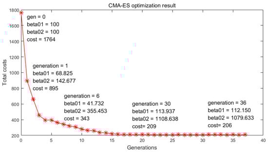
Figure 12.
CMA-ES optimization result.
The optimization process took approximately 40 min. on a Raspberry Pi 3B microcomputer. The hyperparameters are listed in Table 4. When compared to the training process in the simulation environment, the number of sample points and offspring points are greatly reduced to accelerate the training process.
Table 4.
CMA-ES training hyper parameters on real platform.
5.2. Outdoor Flight Experiment Result
Two flight tests are shown in this section. The quadrotor platform, the controller, and the flight performance are shown in Figure 13.
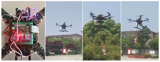
Figure 13.
Outdoor flight experiments.
- (1)
- Attitude Tracking Performance.In this test, a set of experiments are designed in order to evaluate the tracking performance of the proposed method. No external disturbance is added in this test. The desired attitudes are manually controlled with a remote controller, and the flight log data are presented in Figure 14 and Figure 15. According to Figure 14, the actual attitude can track the desired attitude rapidly and smoothly. Figure 15 shows the attitude error are between four degrees during the test.
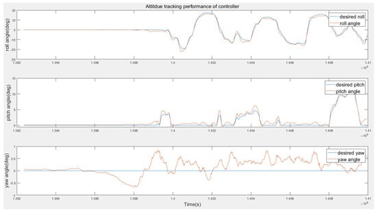 Figure 14. Attitude tracking performance of the RL controller.
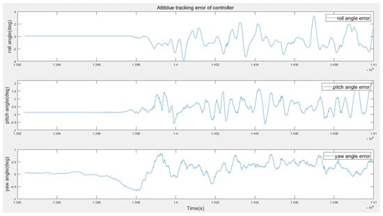 Figure 15. Attitude error of the RL controller.
 - (2)
- Disturbance Rejection Performance.A bottle of water is hung on one side of the drone in this test (see Figure 13). Notably, the water bottle keeps swinging during the flight experiment, which can be considered to be a severe unknown disturbance. Figure 16 shows the tracking performance is still good with the bottle swinging. Figure 17 shows that the maximum attitude error is below four degrees even with severe disturbance.
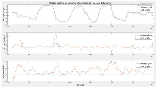 Figure 16. Attitude tracking performance of the RL controller with external disturbance.
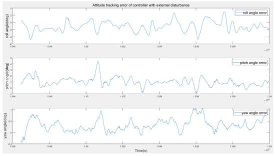 Figure 17. Attitude error of the RL controller with external disturbance.
6. Conclusions
In this paper, we present a single-parameter-tuned attitude control for a quadrotor in the presence of an unknown disturbance, which is, only one tuning parameter is required for each axis. The method is a combination of RL and ADRC. The critical parameters of the system are extracted as CGPs and used to extend the RL state list to improve the robustness of the RL controller. The introduction of mirror sampling and reward shaping eliminate steady-state errors that are incurred using the RL algorithm during continuous control and considerably accelerate the training process. ESOs are designed to estimate external disturbances. A CMA-ES algorithm is developed to automatically tune the ESO parameters, which successfully optimizes the controller performance for both a simulation environment and a real quadrotor platform. The complete controller exhibits excellent performance and remains robust for quadrotors with different physical parameters. When compared to model-based algorithms, such as BS, sliding mode, and H-infinity control algorithms, the method in this paper can be applied on quadrotors with unknown models and parameters meanwhile remain good performance. When compared to PID-based algorithms, our method greatly simplify the parameter tuning work and show better performance.
In our future work, more quadrotor platforms will be tested in order to verify the effectiveness of this single-parameter-tuned quadrotor attitude control system. We will also focus on the improvement of rapidity and stability of the quadrotor attitude control system, and the network training details will be modified further. Moreover, the methods will be tested in quadrotor position control systems.
Author Contributions
Conceptualization, D.H., Z.P. and Z.T.; methodology, D.H.; software, D.H.; validation, D.H.; formal analysis, D.H.; investigation, D.H.; resources, D.H.; data curation, D.H.; writing–original draft preparation, D.H.; writing–review and editing, D.H., Z.P. and Z.T.; visualization, D.H.; supervision, Z.P. and Z.T. All authors have read and agreed to the published version of the manuscript.
Funding
This research received no external funding.
Conflicts of Interest
The authors declare no conflict of interest.
References
- Chovancova, A.; Fico, T.; Duchon, F.; Dekan, M.; Chovanec, L.; Dekanova, M. Control Methods Comparison for the Real Quadrotor on an Innovative Test Stand. Appl. Sci. 2020, 10, 2064. [Google Scholar] [CrossRef]
- Anderson, C. 10 Breakthrough Technologies: Agricultural Drones. MIT Technol. Rev. 2014, 3, 58–60. [Google Scholar]
- Yu, Y.; Yang, S.; Wang, M.; Li, C.; Li, Z. High performance full attitude control of a quadrotor on SO(3). In Proceedings of the 2015 IEEE International Conference on Robotics and Automation (ICRA), Seattle, WA, USA, 26–30 May 2015; pp. 1698–1703. [Google Scholar]
- Xiao, N.S.; Yong, A.Z.; Di, Z. A geometric approach for quadrotor trajectory tracking control. Int. J. Control 2015, 88, 2217–2227. [Google Scholar]
- Hamidreza, J.; Mehran, Z.; Jafar, R.; Amir, A.N. An optimal guidance law applied to quadrotor using LQR method. Trans. Jpn. Soc. Aeronaut. Space Sci. 2010, 179, 32–39. [Google Scholar]
- Liu, C.L.; Pan, J.; Chang, Y.F. PID and LQR trajectory tracking control for an unmanned quadrotor helicopter: Experimental studies. In Proceedings of the 2016 35th Chinese Control Conference (CCC), Chengdu, China, 27–29 July 2016. [Google Scholar]
- Davide, F.; Kevin, K.; Stefano, M.; Dario, F.; Davide, S. The Foldable Drone: A Morphing Quadrotor That Can Squeeze and Fly. Robot. Autom. Lett. 2019, 2, 209–216. [Google Scholar]
- Tarek, M.; Abdelaziz, B. Backstepping control for a quadrotor helicopter. In Proceedings of the 2006 IEEE/RSJ International Conference on Intelligent Robots and Systems, Beijing, China, 9–15 October 2006. [Google Scholar]
- Tarek, M.; Abdelaziz, B. Sliding mode observer and backstepping control for a quadrotor unmanned aerial vehicles. In Proceedings of the 2007 American Control Conference, New York, NY, USA, 9–13 July 2007. [Google Scholar]
- Muñoz, F.; González-Hernández, I.; Salazar, S.; Espinoza, E.S.; Lozano, R. Second order sliding mode controllers for altitude control of a quadrotor UAS: Real-time implementation in outdoor environments. Neurocomputing 2016, 233, 61–71. [Google Scholar] [CrossRef]
- Oualid, D.; AbdurRazzaq, F.; Deok, J.L. Global fast terminal sliding mode control for quadrotor UAV. In Proceedings of the 2017 17th International Conference on Control, Automation and Systems (ICCAS), Jeju, Korea, 18–21 October 2017. [Google Scholar]
- Noormohammadi-Asl, A.; Esrafilian, O.; Arzati, M.A.; Taghirad, H.D. System identification and H-infinity-based control of quadrotor attitude. Mech. Syst. Signal Process. 2020, 135, 106358. [Google Scholar] [CrossRef]
- Liang, X.H.; Wang, Q.; Hu, C.H.; Dong, C.Y. Observer-based H-infinity fault-tolerant attitude control for satellite with actuator and sensor faults. Aerosp. Sci. Technol. 2019, 95, 105424. [Google Scholar] [CrossRef]
- Han, J.Q. From PID to active disturbance rejection control. IEEE Trans. Ind. Electron. 2009, 3, 900–906. [Google Scholar] [CrossRef]
- Madónski, R.; Gao, Z.Q.; Łakomy, K. Towards a turnkey solution of industrial control under the active disturbance rejection paradigm. In Proceedings of the 2015 54th Annual Conference of the Society of Instrument and Control Engineers of Japan (SICE), Hangzhou, China, 28–30 July 2015. [Google Scholar]
- Zhang, Y.; Chen, Z.Q.; Zhang, X.H.; Sun, Q.L.; Sun, M.W. A novel control scheme for quadrotor UAV based upon active disturbance rejection control. Aerosp. Sci. Technol. 2018, 79, 601–609. [Google Scholar] [CrossRef]
- Cai, Z.H.; Lou, J.; Zhao, J.; Wu, K.; Liu, N.J.; Wang, Y.X. Quadrotor trajectory tracking and obstacle avoidance by chaotic grey wolf optimization-based active disturbance rejection control. Mech. Syst. Signal Process. 2019, 128, 636–654. [Google Scholar] [CrossRef]
- Zhang, S.C.; Xue, X.Y.; Chen, C.; Sun, Z.; Sun, T. Development of a low-cost quadrotor UAV based on ADRC for agricultural remote sensing. Int. J. Agric. Biol. Eng. 2019, 4, 82–87. [Google Scholar] [CrossRef]
- Jemin, H.; Inkyu, S.; Roland, S.; Marco, H. Control of a Quadrotor with Reinforcement Learning. IEEE Robot. Autom. Lett. 2017, 4, 2096–2103. [Google Scholar]
- Lin, X.N.; Yu, Y.; Sun, C.Y. Supplementary Reinforcement Learning Controller Designed for Quadrotor UAVs. IEEE Access 2019, 7, 26422–26431. [Google Scholar] [CrossRef]
- Andrew, Y.N.; Hong, J.K.; Michael, J.; Shankar, S. Autonomous helicopter flight via reinforcement learning. In Proceedings of the 9th International Symposium on Experimental Robotics, Singapore, 18–21 June 2004. [Google Scholar]
- Gil, C.R.; Calvo, H.; Sossa, H. Learning an efficient gait cycle of a biped robot based on reinforcement learning and artificial neural networks. Appl. Sci. 2019, 3, 502. [Google Scholar] [CrossRef]
- Wang, Y.; Sun, J.; He, H.B.; Sun, C.Y. Deterministic Policy Gradient with Integral Compensator for Robust Quadrotor Control. IEEE Trans. Syst. Man Cybern. Syst. 2019. [Google Scholar] [CrossRef]
- Nikolaus, H. The CMA Evolution Strategy: A Tutorial. arXiv 2016, arXiv:1604.00772. [Google Scholar]
- Shi, D.J.; Dai, X.H.; Zhang, X.W.; Quan, Q. A practical performance evaluation method for electric multicopters. IEEE/ASME Trans. Mechatron. 2017, 3, 1337–1348. [Google Scholar] [CrossRef]
- David, S.; Guy, L.; Nicolas, H.; Thomas, D.; Daan, W.; Martin, R. Deterministic Policy Gradient Algorithms. In Proceedings of the ICML14: 31st International Conference on International Conference on Machine Learning, Beijing, China, 21–26 June 2014; Volume 32, pp. 387–395. [Google Scholar]
- Diederik, P.K.; Jimmy, L.B. Adam: A Method for Stochastic Optimization. arXiv 2014, arXiv:1412.6980. [Google Scholar]


© 2020 by the authors. Licensee MDPI, Basel, Switzerland. This article is an open access article distributed under the terms and conditions of the Creative Commons Attribution (CC BY) license (http://creativecommons.org/licenses/by/4.0/).