Matching Consignees/Shippers Recommendation System in Courier Service Using Data Analytics

Abstract

The purpose of this research was to create a Matching Consignees/Shippers Recommendation System (MCSRS). We used the association rule to identify product associations, the clustering technique to group shippers and consignees according to behaviors when receiving goods from similar shipper groups, and the decision tree to identify possible matches between shippers and consignees. Finally, Monte Carlo simulation was used to estimate potential revenue. The case study is a courier company in Thailand. The results showed that garment products and clothes were the products with the highest association. Shippers and consignees of these products were segmented according to recency, frequency, monetary factors, number of customers, number of product items, weight, and day. Three rules are proposed that enabled the assignment of 8 consignees to 56 shippers with an estimated increase in revenue by 36%. This approach helps decision-makers to develop an effective cost-saving new marketing, inclusive strategy quickly.

1. Introduction

Recommendation systems (RS) have increasingly been employed owing to technological advancements in understanding individual customer behavior resulting in increased customer satisfaction [1,2,3]. In e-commerce, this commonly applies to product recommendations. An RS suggests products that customers will likely prefer by considering the relationship between a customer’s purchase history and the product’s review rating [4,5]. For example, the popular e-commerce site Amazon has developed an RS by identifying customers who have purchased and rated items. Based on the collaborative filtering algorithm and association rule, Amazon has increased its revenue by 30% [1]. Netflix, the video rental and streaming service, held a competition to improve its RS, called Cinematch. In 2009, a team combined 107 recommendation algorithms resulting in a single prediction, improving predictive accuracy. LinkedIn and Facebook provide recommendations for people you might know, jobs you might like, groups you might want to follow, or companies in which you may be interested. LinkedIn uses Apache Hadoop to build its specialized collaborative-filtering capabilities [2]. This is due to technological advancements that allow data to be collected, stored, and processed effectively, resulting in proactive data that enhances business opportunities, captures new markets and customers, and increases margins. Big data, artificial intelligence, and the Internet of things are examples of how datafication is applied in today’s businesses with many algorithmic approaches available for recommendation engines depending on the type of organization [6].

Data analytics (DA) techniques have been successfully applied in RS to predict user preferences. Suitable algorithms were applied to analyze different characteristics of customer data [3]. DA used in RS includes association rules, clustering techniques, and classification techniques [7], which are used if there are suitable input data [8]. DA algorithms find consumer profiles and purchase patterns in corporate databases that can be used for effective marketing and business decision making. In e-commerce, these procedures can be applied to develop an RS, but they have been extended to deal with specific problems inherent in this kind of application [5]. Likewise, an established database system can apply DA to an RS in other industries, including tourism, hotels, banks, or entertainment [4].

A courier is a company or person responsible for performing shipping services [9]. Courier businesses became a key service industry playing an important role in industrialized economies due to the globalization of e-commerce. The competition in price and quality forces companies to adjust their strategies for new competitive advantages. There are opportunities in courier businesses to utilize data and information of customers and goods which are millions of transactions yearly. The time of delivery, origin, destination, size, weight, and type of goods are recorded and processed around the world [10]. This transaction data can generate at each instance of service activity. The data contain vast numbers of customer profile (e.g., shipper and receiver names, addresses, contacts) and sale transaction details (e.g., date, time, parcel weight, and freight charges). Such profiles analyze a set of behavior-based characteristics, such as shipment preferences, showing what the customer is actually doing. This database can allow businesses to gain information for decision-making as it identifies target customers, ascertains the needs of these customers, and then specifies how the product satisfies these needs. However, it is essential to determine if this information is used effectively or offers operational improvement by developing insights about customers and analyzing new business models. The concrete implementation of RS in the courier business has thus far been lacking because of the limitations of the database structure. However, this study proposes how RS can be used by using DA to suggest potential matches for shippers and consignees.

The case study in this research involves northern Thailand’s largest bus company. The company offers courier services using the available space under routed buses. The service is in high demand due to the growth of e-commerce. The company saw an opportunity to expand its customer base after using a market development strategy based on the Ansoff Matrix [11] to develop new uses for its existing service. Based on existing customer databases, the Matching Consignees/Shippers Recommendation System (MCSRS) is one of the new market development strategies the company has chosen to use. The system explores new business opportunities for matching shippers with consignees by looking for patterns in receiving/sending and whether there is hidden supply and demand data. However, the company first needs to decide on the MCSRS business model’s design before investment to identify demand, target consumers, product recommendations, and whether the business model will work [12].

Many companies use questionnaires to collect data to analyze customer behavior and needs. This can require long periods to compile feedback and may lead to communication problems and increased costs [13]. Conversely, this research aims to develop an MCSRS for courier services using existing data with minimal effort by applying DA. It will be of interest to note whether DA techniques can gain insight into customers’ preferences and define customer demand in the new business. This approach could help managers decide on investment without the need to create a prototype and perform market testing. If the company implements the MCSRS business model, it could introduce suitable shippers to consignees, creating new business partnerships while increasing delivery volume. In addition, shippers and consignees were provided a suggestion of new products and new business partnerships which are most-likely and predictably matched. This study explores whether DA can be used to identify association, raising the following research questions:

RQ1 Which products/items do consignees most often receive together? Which items are likely to be recommended?

RQ2 Which shippers and consignees are the most/least valuable? What are their distinct characteristics?

RQ3 Which shippers and consignees have a greater likelihood of becoming new business partners?

RQ4 Can the matching of consignees and shippers generate revenue?

This paper is organized as follows: Section 2 presents relevant literature. Section 3 describes the research methodology. Section 4 describes the implementation through a case study. Finally, Section 5 presents conclusion and discussion along with the limitations of the study.

2. Literature Review

Understanding customer demand can help a company estimate and manage production capacity, research and development, advertising, and investments [14]. Correctly matching the demand with the right supply can allow businesses to gain customer satisfaction and competitive advantage. Boysen et al. [15] presented a demand and supply matching recommendation for parking spaces, and driver requests in sharing economy using the classification scheme. Products and services also depend on the resources and production capabilities available to the business. A firm needs to know how a new product or service would fit customer demand and company supply [16]. Klassen and Rohleder [17] reported that customer demand influences facility design and equipment in service sectors. To ensure adequate service levels, services that experience large, fast, and unpredictable changes in the market tend to have enough capacity to serve the higher levels of expected demand. Therefore, demand and capacity are generally required simultaneously for decisions. To develop new services efficiently, firms must be able to appropriately identify and understand demand, including customer needs and behavior [18].

The business model should be designed collectively to implement the plan. Business models help decide the structure of components, the relationship between the elements, and the dynamics to plan systematically. The Business Model Canvas developed by Osterwalder and Pigneur [19] defines how companies generate revenue and make a profit through the overall structures of process, customers, suppliers, channels, resources, and capabilities. The critical goal of service businesses is to understand customers and their behavior, necessitating identification of key consumer groups [20], while prioritizing the customer to allocate attention and resources to designated customer groups [13].

Researchers have tried to adapt DA tools for the service industry using association rules, clustering techniques, and decision trees to solve for several objectives. Hung and Zhang [21] conducted three DA techniques to discover various patterns of online behaviors and to predict outcomes. Birant [22] proposed a three-step DA for improved customer satisfaction. Liao et al. [23] used association rules and clustering techniques for mining customer knowledge among online customers. Pitchayadejanant and Nakpathom [24] created association rules and cluster analysis to identify patterns in tourism and to suggest related activities. The literature review in the present study focuses on DA tools that could be used to identify demand for the RS: (1) to identify potential customers, (2) to identify potential products, (3) to predict the suggested matches of shippers with consignees, and (4) to simulate the estimated revenue. Five analysis techniques are reviewed: behavior segmentation, association rules, clustering techniques, decision trees, and Monte Carlo simulation. Each of these is discussed further below.

2.1. Shippers/Consignees Behavior Segmentation

Customer segmentation is the process of dividing customers into similar groups according to certain characteristics. Customer information is examined in order to determine and retain profitable and loyal customers and then to develop an effective marketing strategy for each cluster of customers [25]. In the courier business, there are two types of customers: shippers and consignees. Shippers are direct customers who send their products via a courier. Consignees are indirect customers or customers of those shippers. Many factors need to be considered to correctly segment their behavior [26].

The Recency, Frequency, and Monetary Concept (RFM) was introduced by Bult and Wansbeek [27] and is used to analyze aspects of customer behavior, such as the length of time since last purchase (recency), the number of purchases within a certain time period (frequency), and the amount of money spent over a certain time period (monetary). The integration of RFM and DA techniques has been proposed for different applications, such as identifying customers and analyzing profitability. Aggelis and Christodoulakis [28] applied RFM to measure customer profitability and need for banking services. Khajvand et al. [29] proposed a customer lifetime value for customers of a health and beauty company, using an RFM marketing analysis method for segmentation and adding a parameter (count item). Other research combined DA with RFM, including a self-organizing map [30,31], neural networks and decision trees [32], rough set theory [33], chi-square automatic interaction detection [34], genetic algorithm [35], and sequential pattern mining [36,37].

Several studies have considered different versions of RFM analysis. For example, the Length, Recency, Frequency, and Monetary (LRFM) model was proposed by Wu et al. [38]. In addition to standard variables, this considers the length of the relationship between an organization and customers, with L defined as the number of time periods (e.g., days) from first to last purchase. Alternatively, Hosseini et al. [39] proposed a weighted form of RFM, WRFM, that calculates the weight of RFM through the multiplication of wR, wF, and wM, according to their relative importance, to make intuitive judgments about ranking and ordering. Chen et al. [40] developed an Length, Recency, Frequency, Monetary, and Profit (LRFMP) model for a logistics company to predict customer churn. Other versions include Timely RFM (TRFM), which considers the relationship between product properties and purchase periodicity [41]; Recency, Frequency, Duration and Lifetime (RFDL), which measures the duration of website visits [42]; Frequency, Regency, Amount, and Type of merchandise or service (FRAT), which aims to provide a personalized u-commerce recommendation service [43]; Group-RFM (GRFM), which adds product category groups [44]; Recency, Monetary and Loyalty (RML), which adapts RFM into annual transaction environments; Recency, Frequency, Reach (RFR), proposed for application to social media, where variable examples are the last post for recency, the total number of posts for frequency, and the network of friends for reach [22].

In this study, we applied RFM to the number of customers (NC), the number of product items (NP) [42], weight (W), and day (D) to describe the behavioral patterns of shippers and consignees in the courier business. R is the time between the date of previous services and the reference date. Low recency customers tend to repurchase more than high recency customers [22]. F is the total number of services used within a specific period. M is the total spent in THB over a specific time. NP represents business diversity and reflects the previous history of shippers or customers. For example, a shipper who repeatedly sends the same product to individual customers or many customers may also operate as a manufacturer or a distributor of one specific product. On the other hand, if a shipper sends various types of products, the shipper may be a larger enterprise. NC represents the number of customers served by shippers and denotes the type of business. For example, if a shipper delivers products to many customers, it can be assumed that the shipper works in retailing, wholesaling, or online shopping. W represents the average weight of each delivery, which reflects delivery volume. D represents the average number of days between each transaction. A lower number of days means that sending/receiving occurs more frequently, which could suggest that the customer or shipper is an entrepreneur or business.

2.2. Association Rule

The association rule, an important data mining technique is widely used to extract patterns of interest [45]. It is mainly used to determine relationships between features that occur synchronously in databases and is expressed as X ==> Y. The left part of the rule is the antecedent, and the right is the consequent. Sets X and Y are disjointed, and the same item cannot be found in both the antecedent and consequent. A rule is judged on the basis of its support and confidence levels [46]. Association rules surpass minimum support (Min sup) and minimum confidence (Min conf) thresholds defined by a user [47]. Support determines the frequency of the transaction that satisfies X and Y within the set of all transactions. If a rule has low support, it might be happening simply by chance. Conversely, confidence is the conditional probability that Y will occur, given that X has occurred. Thus, the higher the confidence, the more likely it is for Y to be present in transactions that contain X. Chen et al. [48] proposed an association rule to identify associations between a customer profile and the product items purchased, to establish a method of mining changes in customer behavior. Yoshimura et al. [49] applied an association rule to extract frequent combinations of stores to characterize shoppers’ behaviors. Pitchayadejanant and Nakpathom [24] created an association rule to identify patterns of tourism activities in Thai orchards and to suggest related activities.

The Apriori algorithm provides a basic association rule, reading data once for every iteration [50], while Han et al. [51] proposed an Frequent Pattern Growth (FP-Growth) algorithm to increase the efficiency of the data mining process by scanning the file twice. Their approach is efficiently search frequent itemsets with minimum accesses to the original database. Moreover, it reduces the problem of excessively large amount of candidate itemsets. Many studies have compared the two [52,53,54] and specific adaptive methods have been proposed [55,56,57] to improve efficiency. This study uses FP-Growth as a tool for identifying product recommendations.

2.3. Clustering Technique

A cluster is a collection of data objects that are similar to each other and dissimilar to objects of other clusters [58]. There are several clustering algorithms among which K-means and Hierarchical Clustering method are the two most prominent clustering algorithms. Kaushik and Mathur [59] compared the strengths and weaknesses of K-means and Hierarchical Clustering Techniques. Their study indicated that K-means delivers better performance and is suitable for large datasets. K-means is very sensitive to the choice of a starting point for partitioning items into K initial clusters and is used to assign each record in the dataset to only one initial cluster [60]. Although the major limitation is the requirement of the number of clusters k as an input, there exists a technique to find the suitable number of groups of datasets called “k-optimal” that can yield effective and accurate solutions [61]. Validation studies are conducted using the elbow method, which runs K-means clustering on the dataset for each value of k-optimal. A line chart of the average centroid distance is then plotted for each value of k. If the line chart resembles a knee, then the “bend” represents the optimal value of k [62]. The performance of different clustering methods has been compared in several reports [25,63]. Clustering techniques are widely integrated with RFM concepts for discovering patterns and relationships hidden in datasets. This is not only to develop a product/service to satisfy customers but also to track customer purchasing behaviors and to present distinct products/services for each segment. There are many applications of RFM and clustering techniques in different sectors, including the retail industry [31,64,65], banking [28], patient analytics in dental clinics [38], and e-commerce [23]. The literature also shows that several studies have developed modified K-means approaches that can improve efficiency and run time. However, these may lead to complications, and the procedures are complex when applied to large amounts of data or real data sets. Therefore, this study applies the traditional K-means algorithm because of its efficiency in classifying a large number of continuous numerical values of high dimensions.

2.4. Decision Tree

The decision tree algorithm is a supervised classification technique used to classify unknown patterns or to create a predictive model to divide subjects into groups or predict the values of a target variable. ID3 is the original decision tree method proposed by Quinlan [66] who subsequently proposed C4.5. According to Singh and Gupta [67], the decision trees (i.e., ID3, CART, and C4.5) have different characteristics when applied to different types of data sets. C4.5 can handle numerical attributes and eliminate the ID3 bias by dealing with missing values and noisy data [68]. The performance of decision trees is determined based on the accuracy and confidence of rules. Accuracy is defined on the basis of a confusion matrix for evaluating classification models.

Decision trees are widely used in several sectors. Skrbinjek and Dermol [69] applied decision trees in education to determine the relationship between student satisfaction and their performance in an e-classroom. They proposed five student satisfaction factors: student satisfaction (SATISFACT), grade (GRADE), number of students’ attempts to pass the examination (EXAPPROACH), average student responses, and active engagement (views and posts) (EINVOLV), and student workload (WORKLOAD). Gonoodi et al. [70] used a decision tree algorithm to evaluate risk factors associated with vitamin D deficiency. The model investigated 14 variables, with sensitivity, specificity, accuracy, and receiver operating characteristics used for validation. Sheu et al. [71] applied decision trees to analyze the influences of internal cognition and the external environment on the loyalty of animations, comics, and games (ACG) consumers. Their results were used to suggest policies concerning products’ extensional design, marketing, and CRM in the ACG industry. Hsu and Wang [72] used decision trees to identify and classify patterns in the body shapes of soldiers, generating results that are useful for manufacturers to define a suitable range of clothing sizes and to generate regular size patterns to facilitate production. Mitik et al. [73] proposed a hybrid system, using C4.5 decision trees and Naïve Bayes, to classify customers’ interest in an offered product and clusters for product and channel suggestions. The results increased the overall profit/cost ratio. Tayefi et al. [74] developed a decision tree to identify risk factors associated with hypertension that can be used in programs for hypertension management. Tseng et al. [75] applied a decision tree and artificial neural network analysis to analyze historical cases of oral cancer. Dongming et al. [76] used a decision tree to predict the soil quality grade for precision fertilization in agriculture.

Many studies have applied clustering techniques, decision trees derived from customer demographics, and RFM variables. The integration of decision trees and RFM was studied by Chen et al. [40], who developed a customer churn prediction model using a decision tree. LRFMP variables were also considered and found to have an effect on customer churn. Olson et al. [32] analyzed customers’ possible responses to specific product promotion. They compared three data analytics techniques: logistic regression, decision trees, and neural networks, and discussed the relative tradeoffs among these in the context of customer segmentation. Bunnak et al. [77] applied the RFM concept to determine customer loyalty according to the type of customer. Customer loyalty was partitioned into five classes using a K-means clustering algorithm and customer types (platinum, gold, and silver) were heuristically assigned. A classification system using decision trees was used to determine the loyalty of new future customers. Moedjiono et al. [78] applied K-means clustering with RFM for customer segmentation and decision trees, for internet and cable service providers to identify solvent customers who refused to pay after using services.

2.5. Monte Carlo Simulation

Monte Carlo (MC) simulation relies on repeated random sampling and statistical analysis to compute results [79,80]. It is closely related to random experiments, i.e., experiments for which the specific result is not known in advance [81]. These models typically depend on a number of input parameters, which result in one or more outputs. Mathematical models are used in natural sciences, social sciences, and engineering disciplines to describe interactions in a system of mathematical expressions [82,83].

In MC simulation, each problem is representative of a broad class of similar problems—for a detailed discussion, refer to Glasserman [84]. The technique has been applied in fields such as financial analysis, reliability analysis, Six Sigma, and mathematical and statistical physics. Armaghani et al. [85] applied MC simulation to develop a predictive model for flyrock estimation based on multiple regression analyses. In the present research, MC was used to estimate expected revenue from shippers and consignees through integration with a data mining tool to generate input data before the simulation.

The literature review shows that each tool can deal with the specific problems of several fields and industries. However, this study aims to close these gaps by integrating DA techniques, association rules, clustering techniques, and decision tree for new business development decisions in the logistics business. Therefore, this study implements DA to develop a recommendation approach for matching suitable consignees/shippers using a case study of courier service business. The MCSRS integrates association rules, clustering techniques, and decision tree learning with RFM analysis to better understand the customer behavior. The specific sets of questions are listed in

Table 1. Summary of research questions and selected techniques from the literature review.

Research Question (RQ)	DA Techniques	Description
RQ1 Which products/items do consignees most often receive together? Which items are likely to be recommended?	Association rule FP-Growth	Discover relationships between product categories that are normally or frequently delivered together.
RQ2 Which shippers and consignees are the most/least valuable? What are their distinct characteristics?	Clustering technique K-means R, F, M, NC, NP, W, and D variables	Group customers according to patterns of behavior and target potential customers to provide recommendations.
RQ3 Which shippers and consignees have a greater likelihood of becoming new business partners?	Classification technique Decision tree C4.5 R, F, M, NC, NP, W, and D variables	Learn to predict potential business matches between shippers and consignees.
RQ4 Can the matching of consignees and shippers generate revenue?	Simulation Monte Carlo	Estimate revenue that would be generated to support investment decision-making and to simulate new business scenarios.

.

3. Methodology

The method comprises four steps (Figure 1). Data of 461,708 transactions, involving 94,725 shippers and 137,652 consignees, were obtained from a 2018 sales database. The data were pre-processed and the outliers were detected e.g., the unexpectedly high cargo weight was replaced by the mean of all samples. The redundant attributes e.g., Mr.Brown Emily, Mr BrownEmily, and MrBrown Emily were conformed. Unnecessary attributes such as employee name and payment type were reduced. Thereafter, the data was transformed into a format suitable for association, clustering, and classification. Steps 1–3 were conducted using RapidMiner Studio 9 software and are described below in detail.

3.1. Step 1: Product Association

To identify product associations, rules are extracted from the product category of consignees’ transactions using the FP-Growth algorithm [51]. This involved the following:

(1)

FP-Growth was used to determine items in the set that have been frequently delivered together in a certain fraction of transactions.

(2)

Evaluation of the association rule used Min sup and Min conf thresholds [47] measured by Equations (1) and (2). Thresholds are defined for expected values of minimum revenue.

$$Support \left(X==>Y\right)=\frac{number of transactions with X and Y}{total number of transactions} \le Min sup.$$

(1)

$$Confidence \left(X==>Y\right)= \frac{support \left(X,Y\right)}{support \left(X\right)} \le Min conf.$$

(2)

3.2. Step 2: Shipper/Consignee Clustering

K-means is used to assign each record in the dataset to one initial cluster. Each record is assigned to the cluster to which it is most similar, using a measure of distance or similarity as the Euclidean distance measure, as per Equation (3)

$$Euclidean distance measure \left(d\right)=\sqrt{{\left(a_1-b_1\right)}^2+{\left(a_2-b_2\right)}^2+\dots +{\left(a_n-b_n\right)}^2}$$

(3)

A suitable number of groups of the dataset is referred to as K-optimal, determined by K-means clustering. Validation is conducted by the elbow method, which runs k-means clustering on the dataset for a range of values of k and each value of k. The average distance within the centroid is calculated using Equation (4), where n is the number of dataset points and d is the distance between clustering centroid and dataset point.

$$Average within centroid distance =\frac{d_{1c}+d_{2c}+d_{3c}}{n}$$

(4)

A line chart of the average within the centroid distance is then plotted for each value of k. If the line chart looks like a knee, then the ‘elbow’ of the knee represents the optimal value of k. This idea is similar to a sum of square error [62].

This step divided shippers of Y and consignees of X==>Y into groups with similar R, F, M, NC, NP, W, and D values. Data were partitioned into k clusters using the K-means technique [86]. This involved four sub-steps:

(1)

Determining R, F, M, NC, NP, W, and D variables for each shipper and consignee

(2)

Correlating variables to investigate relationships

(3)

Determining optimal numbers of clusters, with the K-optimal method [62]. The K-means technique was used to cluster a group of Y shippers and X==>Y consignees.

(4)

Analyzing different clusters of Y shippers and screening potential X==>Y consignee clusters.

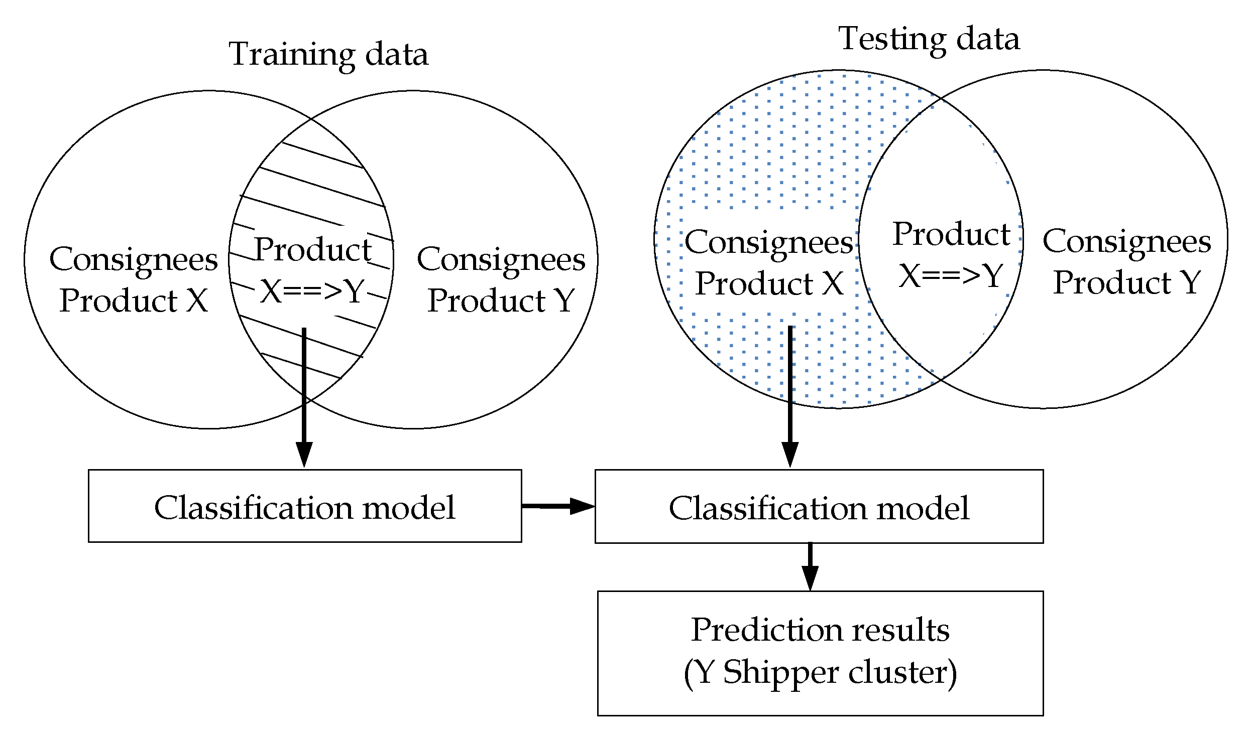
3.3. Step 3: Prediction of Shippers/Consignees Matching

A C 4.5 decision tree was used to identify consignees’ behavior using R, F, M, NC, NP, W, and D variables to predict shipper cluster suggestions. C 4.5 generates a tree by splitting the given data. It calculates overall entropy and information gain for all attributes. The attribute with the highest information gain is then chosen for the decision. At each node of the tree, C 4.5 chooses one attribute that most effectively splits the training data into subsets with the best cut-off point, according to entropy and information gain [22], as per Equations (5) and (6):

$$Entropy \left(t\right)=-{\displaystyle \sum }p\left(\frac{i}{t}\right){\log }_{2}p\left(\frac{i}{t}\right)$$

(5)

$$Information Gain (\nabla )=Entropy \left(parent node\right)-Entropy \left(child node\right)$$

(6)

where $p\left(\frac{i}{t}\right)$ is the fraction of records belonging to class i at a given node t [67]. The process used was as follows:

(1)

Classification of the delivery behavior of X==>Y consignees and Y shipper clusters through a decision tree algorithm. Predictions of X consignees were used as testing data (Figure 2).

(2)

Evaluation of the classification model through 10-fold cross-validation. Accuracy and confidence of rule thresholds were determined for the expected value of minimum revenue in Step 4.

3.4. Step 4: Revenue Simulation

Expected revenue for shippers and consignees in suggested pairings was estimated using the MC and fitness thresholds approach in @Risk 7.6 software. Variables considered are given in Equation (7):

$$Expected revenue=F{\left(x\right)}_{C/G Ratio}\times F{\left(x\right)}_R\times FA\times FC$$

(7)

where $F{\left(x\right)}_{C/G Ratio}$= the revenue ratio of X/Y products (continuous probability distributions), $F{\left(x\right)}_R$ = the total revenue of consignees (continuous probability distributions) in THB, the fitness of association $\left(FA\right)$ = the support value of association * the confidence of association (CA), and the fitness of classification $\left(FC\right)$ = the rule confidence of classification (RC) * the accuracy of classification (AC).

4. Case Study

4.1. The Case and Data Collection

This research used the biggest bus company in northern Thailand, the G Company, for its case study. Over the years, the company has faced strong competition from other types of public transportation, such as taxis, trains, and especially low-cost airlines. The boom in low-cost airlines has affected many market segments owing to competitive prices and promotions that impact customer numbers and profits. To address this crisis, the company has tried to develop two new business units. The first is a charter service, a non-regular route public carrier. The second is a courier service that uses the available space under routed buses. Since 2010, the G Company has provided a port-to-port courier service along its bus routes, using 115 service ports covering 22 provinces from northern to southern Thailand. It provides a courier service as well as packing, short-term warehousing, and door-to-door services in some areas.

The company’s courier service has become an important business with several types of customers, exhibiting a 17.03% revenue growth rate in 2018. The strength of this business is derived from the high frequency of bus travel and low cost, given that the service capitalizes on already available space under passenger service buses. The company has a customer database, providing scope for development of further business opportunities. All sale activities are recorded in the transaction database. However, this is not used for any further analysis at present.

Sales transaction data from 2018 were generated and collected in an Excel spreadsheet. Courier revenue during this year totaled 79 million THB. Attributes collected in the database included shippers’/consignees’ names, dates, times, product group names, product category names, start/destination stations, quantities, weights, freight charges, membership application dates, and payment types (

Table 2. Example of sales transaction data.

Attributes	Data Type	Description and Data Examples
Shipper name	Text	Name of shipper e.g., Mr. Emily Brown
Consignee name	Text	Name of consignee e.g., Mr. John Meily
Date	Numeric	Transaction date e.g., 12/03/2018
Time	Numeric	Transaction time e.g., 10:31:44 AM
Products group name	Nominal	Name of product group e.g., food and drink, clothes, garments, and accessories
Products category name	Nominal	Name of product category e.g., perishable foods, clothes
Start station	Nominal	Name of start station e.g., Chiang Mai
Destination station	Nominal	Name of destination station e.g., Chiang Rai
Quantity	Numeric	Quantity of cargo per transaction
Weight	Numeric	Weight of cargo per transaction (kg) e.g., 15 kg.
Freight charges	Numeric	Freight charges per transaction (THB) e.g., 695 THB.
Membership application date	Numeric	Date of member registration (first transaction) e.g., 05/12/2017
Employee name	Text	Name of sale officer who recorded the transaction
Payment type	Nominal	Payment type e.g., cash, debit, agent

). Products were originally classified into 66 categories (items), then further aggregated into 13 general groups (Figure 3). The products most frequently transported were food and drink (23%); clothes, garments, and accessories (21%); agricultural products (16%); and furniture, décor/kitchenware (10%), respectively.

4.2. Implementation

4.2.1. Identifying Potential Products Using Association Rule

The association rule was used to determine the relationships between product categories and data were separated into two groups—shipper and consignee datasets—to investigate (a) which products are often delivered together and (b) customer behaviors seen when sending/receiving products (

Table 3. Product association rules.

No.	Rule	Support	Confidence
1	Garment products ==> Clothes	0.090	80.81
2	Garments and related products ==> Clothes	0.019	60.79
3	Bags and handbags ==> Clothes	0.018	61.93
4	Car accessories ==> Spare parts	0.010	56.49
5	Garment products ==> Bags and handbags	0.008	87.76
6	Meatballs ==> Perishable foods	0.008	64.21
7	Underwear ==> Clothes	0.007	52.53
8	Computers and spare parts ==> Electronics equipment	0.007	50.00
9	Garment products ==> Garments and related products ==> Clothes	0.006	89.81
10	Sewing equipment ==> Clothes	0.006	75.61
11	Steaks ==> Seasoning ==> Perishable foods	0.006	67.18

). Association diagrams for hidden product categories are shown in Figure 4.

Sequential association rules were applied and Rules 1 through 11 (Table 3) are those with the highest support rates (>0.005). Rule 1 indicates that more than 9% of consignees who receive garment products (in group of handicrafts souvenirs and gifts) and also receive clothes (in group of clothes, garment and accessories) and the data show a confidence level of 80.81%, indicating is a strong relationship between these two items. Rule 2 indicates that 1.9% of consignees who receive garments and related products also receive clothes. Rule 3 indicates that 1.8% of consignees who receive bags and handbags also receive clothes. In this study, Rule 1 is selected as an example rule.

Rule 1: {Garment products ==> Clothes}

Using Rule 1, a list of garment products consignees can be provided to shippers who are clothes suppliers. There can be many shippers and consignees who have not traded with each other. However, not all garment products consignees may want to have clothes delivered. There are 1435 consignees who receive garment products and 14,818 clothes shippers; therefore, investment marketing costs may be high. This necessitates a screening process to identify possible matches. The clustering technique is used for this purpose.

4.2.2. Identifying Potential Customers Using Clustering Technique

Variable Analysis

The clustering technique was applied after generating association rules to identify shippers with similar variables, as defined and calculated in

Table 4. Definition of R, F, M, NC, NP, W, and D variables.

Variables	Definition	Calculation
R (Recency)	Period of time between previous service and set date	Set date—last transaction date
F (Frequency)	Total number of service users within a particular period of time	Count of sale transactions
M (Monetary)	Total THB generated by customer’s service within a particular period of time	Sum of money for each customer
NC (Number of customers)	Number of consignees/shippers	Count of total consignee/shipper customer numbers
NP (Number of product items)	Number of product items	Count of consignee/shipper product items
W (Weight)	Average weight per transaction (kg)	Average weight per transaction (kg)
D (Day)	Interval between transactions (day)	Average number of days between transactions

.

Statistical Correlation Analysis

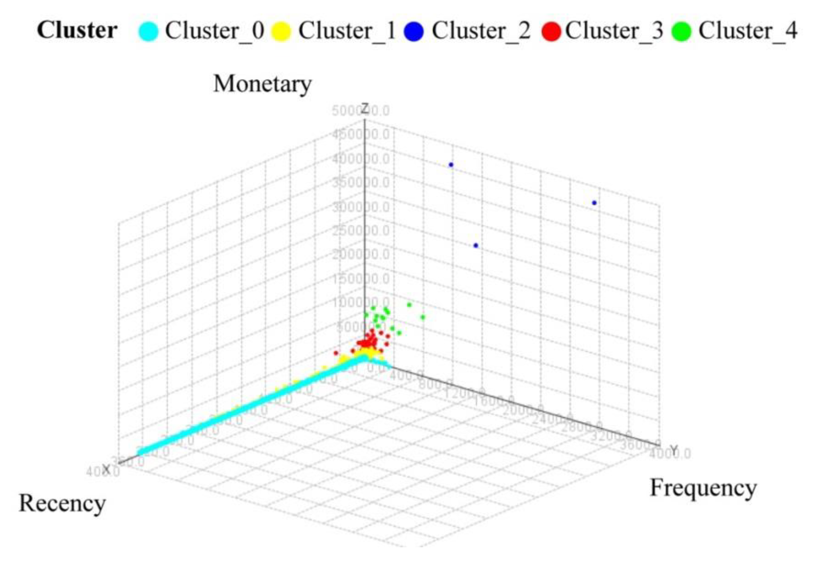
As shown in

Table 5. Statistical correlation between recency (R), frequency (F), monetary (M), number of customers (NC), number of product items (NP), weight (W), and day (D) variables.

	R	F	M	NC	NP	W	D
R	1
F	−0.098	1
M	−0.097	0.895	1
NC	−0.113	0.693	0.686	1
NP	−0.108	0.160	0.154	0.232	1
W	−0.067	0.056	0.127	0.054	0.009	1
D	0.317	−0.145	−0.142	−0.180	−0.203	−0.125	1

, M is related to F with a coefficient of 0.895 and trends in the same direction. However, the lower the value of R, the higher the tendency that such a customer will be a repeat customer, and the lower the value of D, the more frequently a customer uses the service. Overall, however, results show relatively low correlations between variables.

K-means Clustering

Using the product association example of “Garment product ==> Clothes” clothes shippers and garment products and clothes consignees were divided into groups and five clusters were identified. Cluster_0 was the largest group, with 14,534 shippers. This group delivers products twice a year, with an average of 314 THB spent per year. These shippers are not business organizations, as F, NC, and NP are relatively low. Based on D, which was > 272 days on average, this group does not appear to serve regular customers. The next group, Cluster_2, was comprised of three shippers representing the highest average scores of R, F, M, NC, NP, W, and D. The average number of customers was 302, and the average number of products was 15. D was less than 1 day, and the average weight was 36.3 kg. Cluster_2 is the most interesting group with the most business potential. Meanwhile, Clusters_1, 3, and 4 were made up of groups of shippers with higher average scores than Cluster_0 but still lower than in Cluster_2, with 13, 30, and 288 shippers, respectively. For simple ranking, seven variables were normalized, and simple additive weighting (SAW) was used [87]. This indicated that Cluster_2 was the most preferred target, followed by Clusters_4, 3, 1, and 0 (

Table 6. Clustering of 14,818 clothes shippers using Recency, Frequency, and Monetary Concept (RFM) variables.

	R	F	M	NC	NP	W	D	Number in Cluster	Normalized SAW Score	Rank
Cluster_0	160.84	2.32	313.65	1.44	2.09	11.59	272.95	14,534	0.03	5
Cluster_1	27.21	44.01	9920.17	9.34	3.44	39.52	11.75	228	0.12	4
Cluster_2	1.33	1960	408,641	302.00	15	36.28	1.38	3	0.49	1
Cluster_3	7.00	124.98	38,288.36	16.23	4.38	54.68	4.96	40	0.15	3
Cluster_4	1.69	334.15	100,562.4	64.69	9.77	48.06	2.29	13	0.22	2
Total	158.20	3.98	734.59	1.72	2.12	12.17	267.92	14,818	1

). Consignees who receive garment products and clothes were also clustered. Of 2139 consignees, 236 were targeted as potential customers.

Figure 5 shows the 3D scatter plot of RFM values for the various clusters, with a higher RFM indicating more regular customers. Cluster_2 consists of shippers who are more loyal in terms of the frequency of service usage or the amount of money spent on the company’s services. This group is followed by Clusters_4, 3, 1, and 0, with the latter comprised of one-time customers. Variables NC, NP, W, and D were used to analyze shipping to gain insight into behavior, type or size of business, and to provide recommendations for shippers and customers. Figure 6 shows scatter plots for clothes shipper clusters. Most clusters have NC < 50, with the exception of Clusters_2 and 4, which have NC > 100. The numbers of products vary with each cluster. Clusters_1, 2, 3, and 4, however, have a clear pattern for W and D, in contrast to Cluster_0.

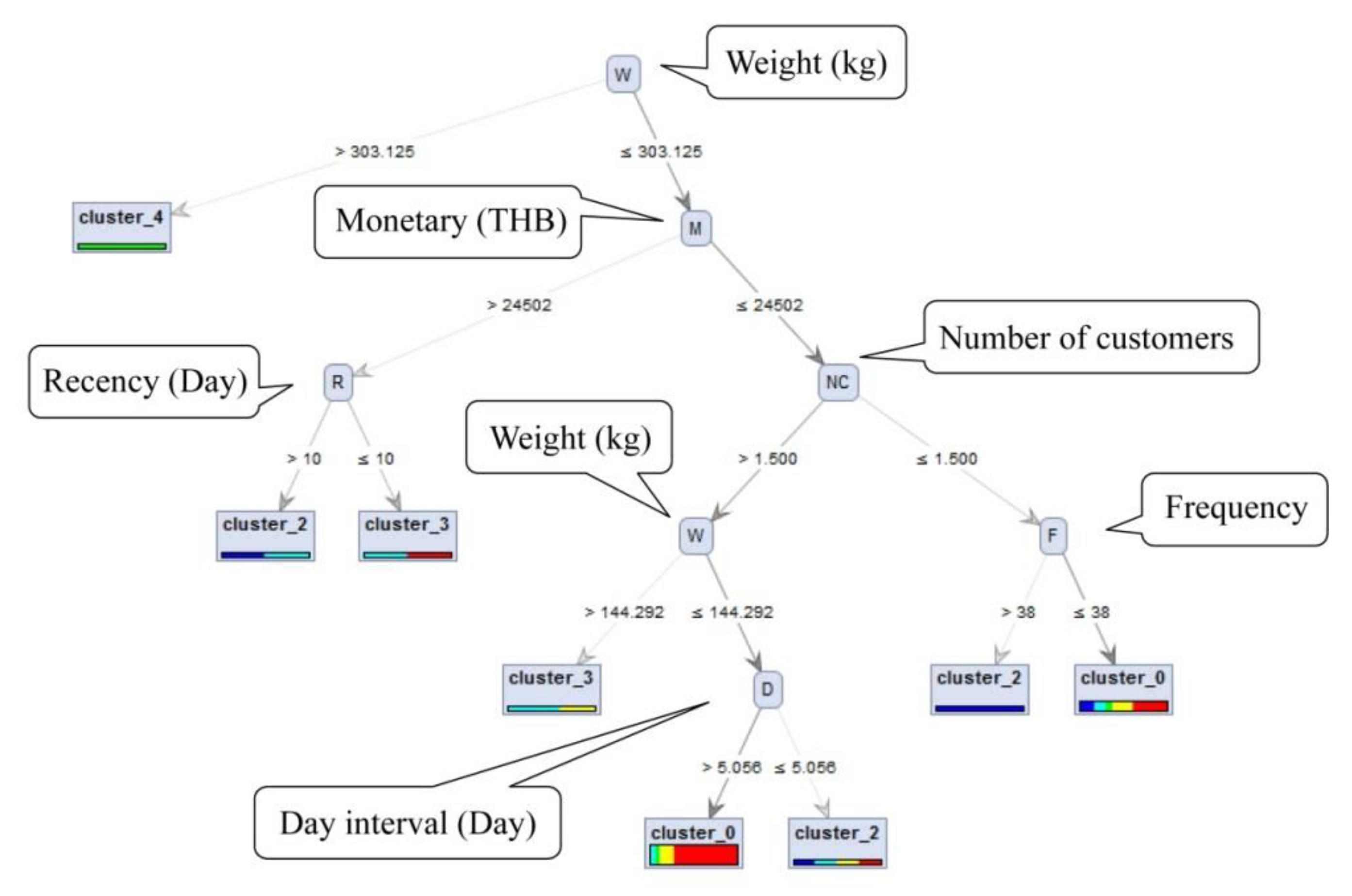
4.2.3. Predicting Possible Matching of Shippers and Consignees Using Decision Tree

Shippers in Cluster_2 had the greatest potential for new business. However, it was necessary to estimate how many matching pairs could be created with the RS and at what level of accuracy. Decision tree learning was used to discover product delivery behavior and to forecast which groups of customers are likely to acquire various products. The dataset used for the behavioral study was obtained from training and testing data (Figure 2). Training data included the data of 263 consignees who received garment products and clothes over 867 transactions. This data was later used for the creation of the classification model. Testing data included 1435 customers of garment products (those who have never received clothes). The model was validated with 10-fold cross-validation. Model efficiency was determined by the number of correct forecasts made in every class. The model learned and predicted the behavior of customers who had never received clothes with an accuracy of 62.40, resulting in eight forecasting rules (Figure 7).

Rules were then selected based on the rule’s level of confidence, the value of the cluster, and the number of members in a cluster, among other factors. Examples of three rules are as follows:

• Rule 1: if {Weight > 303.13 kg} then cluster_4
• Rule 7: if {Weight ≤ 303.13 kg} and {Monetary ≤ 24,502 THB} and {Number of customers ≤ 1.5} and {Frequency > 38} then cluster_2
• Rule 4: if {144.30 kg < Weight ≤ 303.13 kg} and {Monetary ≤ 24,502 THB} and {Number of customers > 1.5} then cluster_3

Rule 1 suggests matching 1 consignee to 13 shippers with confidence level 100%. This rule applies to ‘big lot receivers’ who receive products with an average shipping weight > 303.13 kg and was suggested to 13 shippers in Cluster_4. These are clothes shippers who send high weight and high-frequency deliveries to a number of customers and with a variety of product items (positioning in rank 2). New consignees with parameters within this behavior range can also be suggested to shippers in Cluster_4.

Rule 7 suggests matching 1 consignee to 3 shippers with confidence level 100%. This rule applies to ‘high-frequency receivers’ who receive garment products with average weight < 303.13 kg, with < 24,502 THB spent per year, and with > 2 deliveries/week but a lower weight than the ‘big lot receiver group.’ This consignee group was suggested for 3 shippers in Cluster_2. These rank 1 clothes shippers send high-frequency, high-weight deliveries, have a high number of customers, and manage a variety of product items. New consignees with parameters within this range of behavior, can be suggested to shippers in Cluster_2.

Rule 4 suggests matching 6 consignees to 40 shippers with confidence level 60%. It applies to ‘moderate weight and frequency’ consignees who received garment products from > 1 shipper, with an average shipment weight of 144.30–303.13 kg, with < 24,502 THB spent per year. This group was suggested to 40 shippers in Cluster_3. These are clothes shippers who are positioned in rank 3. New consignees positioned within this range of behavior can be suggested to the 40 shippers in Cluster_3.

Consignees grouped according to Rules 1, 7, and 4 were segmented by F and W, as shown in Figure 8.

4.2.4. Simulating Expected Revenue Using Monte Carlo Simulation

MC simulation was used for dimensional analysis of revenue simulation with @RISK software. Three rules were used to evaluate the feasibility of reaching the expected revenue level, a minimum base requirement when assessing the fitness of models. Variables considered are given in Equation (7)

The $F{\left(x\right)}_{C/G Ratio}$ is taken from the distribution fitting of 2400 consignees in a revenue ratio of clothes/garment products. $F{\left(x\right)}_R$ is taken from the total revenue distribution fitting of consignee numbers according to the rule. SA and CA are derived from Table 3. RC was derived from

Table 7. Classification rules extracted through the decision tree model.

No	Classification Rule	Prediction Shipper Cluster	Number of Consignees in Rule	Number of Shippers in a Cluster	Confidence of Rule-Based Classifier	Accuracy	Association Support
1	W > 303.13	Cluster_4	1	13	100%	62.40%	9%
2	W ≤ 303.13 M > 24,502 R > 10	Cluster_2	0	3	50%
3	W ≤ 303.13 M > 24,502 R ≤ 10	Cluster_3	0	40	50%
4	W ≤ 303.13 M ≤ 24,502 NC > 1.5 W > 144.30	Cluster_3	6	40	60%
5	W ≤ 303.13 M ≤ 24,502 NC > 1.5 W ≤ 144.30 D > 5.1	Cluster_0	381	14,534	72%
6	W ≤ 303.13 M ≤ 24,502 NC > 1.5 W ≤ 144.30 D ≤ 5.1	Cluster_2	12	3	25%
7	W ≤ 303.13 M ≤ 24,502 NC ≤ 1.5 F > 38	Cluster_2	1	3	100%
8	W ≤ 303.13 M ≤ 24,502 NC ≤ 1.5 F ≤ 38	Cluster_0	1034	14,534	39%

, while AC was 0.624.

Table 8. Probability distribution functions of input parameters.

Rule	Consignees: Shippers	$\mathit{F}{\left(\mathit{x}\right)}_{\mathit{C}/\mathit{G} \mathit{R}\mathit{a}\mathit{t}\mathit{i}\mathit{o}}$	$\mathit{F}{\left(\mathit{x}\right)}_{\mathit{R}}$	Fitness of Association Model		Fitness of Classification Model		Expected Revenue (THB)
				SA	CA	RC	AC
1	1:13	Triang (4.05, 6.5015) (N = 2400)	3884	0.09	0.80	1	0.624	1038
7	1:3		11,429			1		3063
4	6:40		Pareto (0.9681, 1076) (N = 6)			0.60		12,266

shows the distribution model of expected revenue obtained using MC modeling, together with summary input and output parameters. For example, expected revenue of 1038 THB for Rule 1 was obtained based on $F{\left(x\right)}_{C/G Ratio}$ of Triang (4.05, 6.5015), $F{\left(x\right)}_R$ of 3884, SA of 0.09, CA of 0.8, RC of 1, and AC of 0.624.

Predictions of the expected revenue result from simulations of 10,000 iterations and

Table 9. Obtained minimum, mean, and maximum expected revenue (THB) within 90% confidence level using MC modeling of Rules 1, 7, 4, and the total.

Rule	Minimum, Mean, Maximum Expected Revenue (THB)	Continuous Distribution Functions
1	(192, 1038, 2675)	Lognorm (1082, 939.8)
7	(558, 3063, 8161)	Lognorm (3186.2, 2789.7)
4	(334, 12,266, 22,200)	Pearson5 (1.095, 1561)
Total	(2380, 16,368, 27,500)	Pearson5 (2.0665, 10556)

shows the results of MC modeling (90% confidence level). For Rule 1, the Lognorm (1082, 939.8) was the best-fitting model and a value of 1038 THB/year was simulated as the most likely expected revenue with a range of 192–2675 THB/year. For Rule 7, the Lognorm (3186.2, 2789.7) was also the best-fitting model, with expected revenue of 3063 THB/year and a range of 558–8161 THB/year. For Rule 4, the most likely expected revenue was 12,266 THB, and a range of 334–22,200 THB/year. Based on these rules, revenue is expected to grow by 16,368 THB/year, equivalent to a 36% revenue increase from eight consignees. Even more revenue can be generated by considering all rules and all product categories and creating classification rules for suggesting supply-demand relationships.

5. Conclusions and Discussion

The purpose of this study was to demonstrate the benefits of implementing DA to create a model for pairing consignees and shippers for a Thai courier service. DA was performed using a database of 461,708 sales transactions between 94,725 shippers and 137,652 consignees. To answer RQ1, the association rule was used to learn which categories of products consignees often received together and which shippers could be matched with consignees based on the type of products received. Our results suggested pairing clothes shippers with garment product consignees identified from a total of 1435 garment product consignees and 14,818 clothes shippers. The clustering technique was used to answer RQ2 to identify customers with similar behaviors in order to link five identified shipper clusters to the appropriate consignee groups. To determine the answer to RQ3, a decision tree was used to classify consignees based on behavior patterns exhibited when receiving goods from similar shipper groups. Three rules were used to link 8 consignees to 56 shippers (Figure 9). Finally, RQ4 was answered by using MC simulation to predict an estimated revenue increase of 36%, or 16,368 THB/year. This approach could recommend new products to new shippers and consignees without affecting the original consignee-shipper relationships. However, the results presented here only consider a pair of product categories and three prediction rules. If all product categories were considered, this could generate an additional 6.6% of total revenue (5.2 million THB/year) and an additional 31,000 transactions.

The demonstrated approach successfully used DA techniques in identify suitable pairings, which can help companies to segment customers according to behavioral characteristics while prioritizing customers via appropriate marketing channels. Additionally, the approach assists in the prediction of the expected revenue, allowing a company to make informed investment decisions. This approach could be applied to other courier businesses. Thailand has many such businesses, accounting for a market value of up to 30 billion THB; as such, this approach could have significant economic impact.

However, this study had limited data (461,708 transactions from one year). Additionally, the categories of products used were rather broad. More specific identification of products would deliver more accurate results.

Future research can consider an analysis of other product pairs that could result in increased revenue. Model validation can be conducted by interviewing consignees and determining if they would be interested in these suggestions. This would help confirm that the approach is credible and usable in real situations.

References

1. Linden, G.; Smith, B.; York, J. Amazon.com recommendations: Item-to-item collaborative filtering. IEEE Internet Comput. 2003, 7, 76–80. [Google Scholar] [CrossRef] [Green Version]
2. Chajri, M.; Fakir, M. Application of Data Mining in e-Commerce. J. Inf. Technol. Res. 2014, 7, 79–91. [Google Scholar] [CrossRef]
3. Osadchiy, T.; Poliakov, I.; Olivier, P.; Rowland, M.; Foster, E.; Rowland, M. Recommender system based on pairwise association rules. Expert Syst. Appl. 2019, 115, 535–542. [Google Scholar] [CrossRef]
4. Tewari, A.S.; Barman, A.G. Sequencing of items in personalized recommendations using multiple recommendation techniques. Expert Syst. Appl. 2018, 97, 70–82. [Google Scholar] [CrossRef]
5. Lu, Q.; Guo, F. Personalized information recommendation model based on context contribution and item correlation. Measurement 2019, 142, 30–39. [Google Scholar] [CrossRef]
6. Erevelles, S.; Fukawa, N.; Swayne, L. Big Data consumer analytics and the transformation of marketing. J. Bus. Res. 2016, 69, 897–904. [Google Scholar] [CrossRef]
7. Ramamohan, Y.; Vasantharao, K.; Chakravarti, C.K.; Ratnam, A.S.K. A study of data mining tools in knowledge discovery process. Int. J. Soft Comput. Eng. (IJSCE) 2012, 2, 2231–2307. [Google Scholar]
8. Sopadang, A.; Cho, B.R.; Leonard, M.S. Development of a Scaling Factor Identification Method Using Design of Experiments for Product-Family-Based Product and Process Design. Qual. Eng. 2002, 14, 319–329. [Google Scholar] [CrossRef]
9. Gulc, A. Courier service quality from the clients’ perspective. Eng. Manag. Prod. Serv. 2017, 9, 36–45. [Google Scholar] [CrossRef] [Green Version]
10. Ben Ayed, A.; Ben Halima, M.; Alimi, M.A. Big data analytics for logistics and transportation. In Proceedings of the 2015 4th International Conference on Advanced Logistics and Transport (ICALT), Valenciennes, France, 20–22 May 2015; pp. 311–316. [Google Scholar]
11. Ansoff, H.I. Strategies for diversification. Harv. Bus. Rev. 1957, 35, 113–124. [Google Scholar]
12. Dudin, M.; Lyasnikov, N.V.; Leont’Eva, L.S.; Reshetov, K.; Sidorenko, V.N. Business Model Canvas as a Basis for the Competitive Advantage of Enterprise structures in the Industrial Agriculture. Biosci. Biotechnol. Res. Asia 2015, 12, 887–894. [Google Scholar] [CrossRef]
13. Huang, C.-C.; Liang, W.-Y.; Wen, D.-W.; Ting, P.-H.; Shen, M.-Y. Qualitative analysis of big data in the service sectors. Serv. Ind. J. 2018, 1–19. [Google Scholar] [CrossRef]
14. Ellis, J.A.; Fee, C.E.; Thomas, S.E. Proprietary Costs and the Disclosure of Information about Customers. J. Account. Res. 2012, 50, 685–727. [Google Scholar] [CrossRef]
15. Boysen, N.; Briskorn, D.; Schwerdfeger, S. Matching supply and demand in a sharing economy: Classification, computational complexity, and application. Eur. J. Oper. Res. 2019, 278, 578–595. [Google Scholar] [CrossRef]
16. Dougherty, D. A practice-centered model of organizational renewal through product innovation. Strat. Manag. J. 1992, 13, 77–92. [Google Scholar] [CrossRef]
17. Klassen, K.; Rohleder, T. Combining Operations and Marketing to Manage Capacity and Demand in Services. Serv. Ind. J. 2001, 21, 1–30. [Google Scholar] [CrossRef]
18. Chen, L.-F.; Chen, S.-C.; Su, C.-T. An innovative service quality evaluation and improvement model. Serv. Ind. J. 2017, 38, 228–249. [Google Scholar] [CrossRef]
19. Osterwalder, A.; Pigneur, Y. Business Model Generation: A Handbook for Visionaries, Game Changers, and Challengers; John Wiley and Sons: Hoboken, NJ, USA, 2010; p. 288. [Google Scholar]
20. Zolnowski, A.; Weiss, C.; Böhmann, T. Representing Service Business Models with the Service Business Model Canvas—The Case of a Mobile Payment Service in the Retail Industry. In Proceedings of the 2014 47th Hawaii International Conference on System Sciences, Waikoloa, HI, USA, 6–9 January 2014; pp. 718–727. [Google Scholar]
21. Hung, J.L.; Zhang, K. Revealing online learning behaviors and activity patterns and making predictions with data mining techniques in online teaching. MERLOT J. Online Learn. Teach. 2008, 4, 425–437. [Google Scholar]
22. Birant, D. Data Mining Using RFM Analysis. In Knowledge-Oriented Applications in Data Mining; IntechOpen: London, UK, 2011; pp. 91–108. [Google Scholar]
23. Liao, S.-H.; Chu, P.-H.; Chen, Y.-J.; Chang, C.-C. Mining customer knowledge for exploring online group buying behavior. Expert Syst. Appl. 2012, 39, 3708–3716. [Google Scholar] [CrossRef]
24. Pitchayadejanant, K.; Nakpathom, P. Data mining approach for arranging and clustering the agro-tourism activities in orchard. Kasetsart J. Soc. Sci. 2018, 39, 407–413. [Google Scholar] [CrossRef]
25. Christy, A.J.; Umamakeswari, A.; Priyatharsini, L.; Neyaa, A. RFM ranking—An effective approach to customer segmentation. J. King Saud Univ. Comput. Inf. Sci. 2018. [Google Scholar] [CrossRef]
26. Jintana, J.; Mori, T. Customer clustering for a new method of marketing strategy support within the courier business. Acad. Book Chapter 2019, 31, 1–19. [Google Scholar]
27. Bult, J.R.; Wansbeek, T. Optimal Selection for Direct Mail. Mark. Sci. 1995, 14, 378–394. [Google Scholar] [CrossRef]
28. Aggelis, V.; Christodoulakis, D. Customer clustering using RFM analysis. In Proceedings of the 9th World Scientific and Engineering Academy and Society (WSEAS) International Conference on Computers (ICCOMP’05), Stevens Point, WI, USA, 14 July 2005; pp. 1–5. [Google Scholar]
29. Khajvand, M.; Zolfaghar, K.; Ashoori, S.; Alizadeh, S. Estimating customer lifetime value based on RFM analysis of customer purchase behavior: Case study. Procedia Comput. Sci. 2011, 3, 57–63. [Google Scholar] [CrossRef] [Green Version]
30. Li, S.-T.; Shue, L.-Y.; Lee, S.-F. Business intelligence approach to supporting strategy-making of ISP service management. Expert Syst. Appl. 2008, 35, 739–754. [Google Scholar] [CrossRef]
31. Daoud, R.A.; Amine, A.; Bouikhalene, B.; Lbibb, R. Combining RFM model and clustering techniques for customer value analysis of a company selling online. In Proceedings of the 2015 IEEE/ACS 12th International Conference of Computer Systems and Applications (AICCSA), Marrakech, Morocco, 17–20 November 2015; pp. 1–6. [Google Scholar]
32. Olson, D.L.; Cao, Q.; Gu, C.; Lee, D. Comparison of customer response models. Serv. Bus. 2009, 3, 117–130. [Google Scholar] [CrossRef]
33. Cheng, C.-H.; Chen, Y.-S. Classifying the segmentation of customer value via RFM model and RS theory. Expert Syst. Appl. 2009, 36. [Google Scholar] [CrossRef]
34. Mccarty, J.A.; Hastak, M. Segmentation approaches in data-mining: A comparison of RFM, CHAID, and logistic regression. J. Bus. Res. 2007, 60, 656–662. [Google Scholar] [CrossRef]
35. Chan, C.C.H. Intelligent value-based customer segmentation method for campaign management: A case study of automobile retailer. Expert Syst. Appl. 2008, 34, 2754–2762. [Google Scholar] [CrossRef]
36. Chen, Y.-L.; Kuo, M.-H.; Wu, S.-Y.; Tang, K. Discovering recency, frequency, and monetary (RFM) sequential patterns from customers’ purchasing data. Electron. Commer. Res. Appl. 2009, 8, 241–251. [Google Scholar] [CrossRef]
37. Liu, D.-R.; Lai, C.-H.; Lee, W.-J. A hybrid of sequential rules and collaborative filtering for product recommendation. Inf. Sci. 2009, 179, 3505–3519. [Google Scholar] [CrossRef]
38. Wu, H.-H.; Lin, S.-Y.; Liu, C.-W. Analyzing Patients’ Values by Applying Cluster Analysis and LRFM Model in a Pediatric Dental Clinic in Taiwan. Sci. World J. 2014, 2014, 1–7. [Google Scholar] [CrossRef]
39. Hosseini, S.M.S.; Maleki, A.; Gholamian, M.R. Cluster analysis using data mining approach to develop CRM methodology to assess the customer loyalty. Expert Syst. Appl. 2010, 37, 5259–5264. [Google Scholar] [CrossRef]
40. Chen, K.; Hu, Y.-H.; Hsieh, Y.-C. Predicting customer churn from valuable B2B customers in the logistics industry: A case study. Inf. Syst. e-Bus. Manag. 2014, 13, 475–494. [Google Scholar] [CrossRef]
41. Lee, L.H.L.F.M.; Liu, W.J. The timely product recommendation based on RFM method. In Proceedings of the International Conference on Business and Information, Singapore, 12–14 July 2006. [Google Scholar]
42. Sung, C.; Zhang, B.; Higgins, C.Y.; Choe, Y. Data-Driven Sales Leads Prediction for Everything-as-a-Service in the Cloud. In Proceedings of the 2016 IEEE International Conference on Data Science and Advanced Analytics (DSAA), Montreal, QC, Canada, 17–19 October 2016; pp. 557–563. [Google Scholar]
43. Cho, Y.S.; Ryu, K.H.; Ryu, K.S.; Moon, S.C. Personalized u-commerce recommending service using weighted sequential pattern with time-series and FRAT method. In Proceedings of the 2014 IEEE International Conference on Management of Innovation and Technology, Singapore, 23–25 September 2014; pp. 295–300. [Google Scholar]
44. Chang, H.-C.; Tsai, H.-P. Group RFM analysis as a novel framework to discover better customer consumption behavior. Expert Syst. Appl. 2011, 38, 14499–14513. [Google Scholar] [CrossRef]
45. Agrawal, R.; Srikant, R. Fast algorithms for mining association rules. In Proceedings of the 20th International Conference on Very Large Databases (VLDB), Santiago, Chile, 12–15 September 1994; pp. 487–499. [Google Scholar]
46. Plasse, M.; Niang, N.; Saporta, G.; Villeminot, A.; Leblond, L. Combined use of association rules mining and clustering methods to find relevant links between binary rare attributes in a large data set. Comput. Stat. Data Anal. 2007, 52, 596–613. [Google Scholar] [CrossRef]
47. Song, H.S.; Kim, J.K.; Kim, S.H. Mining the change of customer behavior in an internet shopping mall. Expert Syst. Appl. 2001, 21, 157–168. [Google Scholar] [CrossRef]
48. Chen, M.; Chiu, A.; Chang, H.-H. Mining changes in customer behavior in retail marketing. Expert Syst. Appl. 2005, 28, 773–781. [Google Scholar] [CrossRef]
49. Yoshimura, Y.; Sobolevsky, S.; Hobin, J.N.B.; Ratti, C.; Blat, J. Urban association rules: Uncovering linked trips for shopping behavior. Environ. Plan. B Urban Anal. City Sci. 2016, 45, 367–385. [Google Scholar] [CrossRef]
50. Agrawal, R.; Imielinski, T.; Swami, A. Mining association rules between sets of items in large databases. ACM SIGMOD Rec. 1993, 22, 207–216. [Google Scholar] [CrossRef]
51. Han, J.; Pei, J.; Yin, Y. Mining frequent patterns without candidate generation. ACM SIGMOD Rec. 2000, 29, 1–12. [Google Scholar] [CrossRef]
52. Zhang, W.; Liao, H.; Zhao, N. Research on the FP Growth Algorithm about Association Rule Mining. In Proceedings of the 2008 International Seminar on Business and Information Management, Wuhan, China, 19 December 2008; pp. 315–318. [Google Scholar]
53. Kumar, B.S.; Rukmani, K.V. Implementation of web usage mining using Apriori and FP growth algorithms. Int. J. Adv. Netw. Appl. 2010, 1, 400–404. [Google Scholar]
54. Hunyadi, D. Performance comparison of Apriori and FP-Growth algorithms in generating association rules. In Proceedings of the 5th European Computing Conference (ECC’11), Paris, France, 28–30 April 2011; pp. 376–381. [Google Scholar]
55. Lin, K.-C.; Liao, I.-E.; Chen, Z.-S. An improved frequent pattern growth method for mining association rules. Expert Syst. Appl. 2011, 38, 5154–5161. [Google Scholar] [CrossRef]
56. Yang, W.; Hui, L.; Zhang, N.; Fu, Y. An Improved Incremental Queue Association Rules for Mining Mass Text. In Proceedings of the 2016 International Symposium on Computer, Consumer and Control (IS3C), Xi’an, China, 4–6 July 2016; pp. 447–450. [Google Scholar]
57. Wang, B.; Chen, D.; Shi, B.; Zhang, J.; Duan, Y.; Chen, J.; Hu, R. Comprehensive Association Rules Mining of Health Examination Data with an Extended FP-Growth Method. Mob. Netw. Appl. 2017, 22, 267–274. [Google Scholar] [CrossRef]
58. Han, J.; Kamber, M. Data Mining Concepts and Techniques; Elsevier: Amsterdam, The Netherlands, 2001. [Google Scholar]
59. Kaushik, M.; Mathur, B. Comparative study of K-means and hierarchical clustering techniques. Int. J. Softw. Hardw. Res. Eng. 2014, 2, 93–98. [Google Scholar]
60. MacQueen, J. Some methods for classification and analysis of multivariate observations. In Proceedings of the Fifth Berkeley Symposium On Mathematical Statistics And Probability, Berkeley, CA, USA, 21 June–18 July 1965 and 27 December 1965–7 January 1966; University of California Press: Berkeley, CA, USA, 1967; Volume 1, pp. 281–297. [Google Scholar]
61. Abbas, O.A. Comparisons between Data Clustering Algorithms. Int. Arab J. Inf. Technol. 2008, 5, 320–325. [Google Scholar]
62. Liu, C.C.; Chu, S.W.; Chan, Y.K.; Yu, S.S. A Modified K-Means Algorithm—Two-Layer K-Means Algorithm. In Proceedings of the 2014 Tenth International Conference on Intelligent Information Hiding and Multimedia Signal Proceedings, Kitakyushu, Japan, 27–29 August 2014; pp. 447–450. [Google Scholar]
63. Shah, S.; Singh, M. Comparison of a Time Efficient Modified K-mean Algorithm with K-Mean and K-Medoid Algorithm. In Proceedings of the 2012 International Conference on Communication Systems and Network Technologies, Rajkot, India, 11–13 May 2012; pp. 435–437. [Google Scholar]
64. Chen, D.; Sain, S.L.; Guo, K. Data mining for the online retail industry: A case study of RFM model-based customer segmentation using data mining. J. Database Mark. Cust. Strat. Manag. 2012, 19, 197–208. [Google Scholar] [CrossRef]
65. Parvaneh, A.; Tarokh, M.; Abbasimehr, H. Combining data mining and group decision making in retailer segmentation based on LRFMP variables. Int. J. Ind. Eng. Prod. Res. 2014, 25, 197–206. [Google Scholar]
66. Quinlan, J.R. Induction of decision trees. Mach. Learn. 1986, 1, 81–106. [Google Scholar] [CrossRef] [Green Version]
67. Singh, S.; Gupta, P. Comparative study ID3, cart and C4. 5 decision tree algorithm: A survey. Int. J. Adv. Inf. Sci. Technol. 2014, 27, 97–103. [Google Scholar]
68. Song, Y.-Y.; Lu, Y. Decision tree methods: Applications for classification and prediction. Shanghai Arch Psychiatry 2015, 27, 130–135. [Google Scholar] [PubMed]
69. Skrbinjek, V.; Dermol, V. Predicting students’ satisfaction using a decision tree. Tert. Educ. Manag. 2019, 25, 101–113. [Google Scholar] [CrossRef]
70. Gonoodi, K.; Tayefi, M.; Saberi-Karimian, M.; Amirabadizadeh, A.; Darroudi, S.; Farahmand, S.K.; Abasalti, Z.; Moslem, A.; Nematy, M.; Ferns, G.A.; et al. An assessment of the risk factors for vitamin D deficiency using a decision tree model. Diabetes Metab. Syndr. Clin. Res. Rev. 2019, 13, 1773–1777. [Google Scholar] [CrossRef] [PubMed]
71. Sheu, J.-J.; Chu, K.-T.; Wang, S.-M. The associate impact of individual internal experiences and reference groups on buying behavior: A case study of animations, comics, and games consumers. Telemat. Inform. 2017, 34, 314–325. [Google Scholar] [CrossRef]
72. Hsu, C.-H.; Wang, M.-J.J. Using decision tree-based data mining to establish a sizing system for the manufacture of garments. Int. J. Adv. Manuf. Technol. 2004, 26, 669–674. [Google Scholar] [CrossRef]
73. Mitik, M.; Korkmaz, O.; Karagoz, P.; Toroslu, I.H.; Yucel, F. Data Mining Approach for Direct Marketing of Banking Products with Profit/Cost Analysis. Rev. Socionetwork Strat. 2017, 11, 17–31. [Google Scholar] [CrossRef]
74. Tayefi, M.; Esmaeili, H.; Karimian, M.S.; Zadeh, A.A.; Ebrahimi, M.; Safarian, M.; Nematy, M.; Parizadeh, S.M.R.; Ferns, G.A.; Ghayour-Mobarhan, M. The application of a decision tree to establish the parameters associated with hypertension. Comput. Methods Programs Biomed. 2017, 139, 83–91. [Google Scholar] [CrossRef]
75. Tseng, W.-T.; Chiang, W.-F.; Liu, S.-Y.; Roan, J.; Lin, C.-N. The Application of Data Mining Techniques to Oral Cancer Prognosis. J. Med Syst. 2015, 39, 59. [Google Scholar] [CrossRef]
76. Dongming, L.; Yan, L.; Chao, Y.; Chaoran, L.; Huan, L.; Lijuan, Z. The application of decision tree C4.5 algorithm to soil quality grade forecasting model. In Proceedings of the 2016 First IEEE International Conference on Computer Communication and the Internet (ICCCI), Wuhan, China, 13–15 October 2016; pp. 552–555. [Google Scholar]
77. Bunnak, P.; Thammaboosadee, S.; Kiattisin, S. Applying Data Mining Techniques and Extended RFM Model in Customer Loyalty Measurement. J. Adv. Inf. Technol. 2015, 238–242. [Google Scholar] [CrossRef]
78. Moedjiono, S.; Fransisca, F.; Kusdaryono, A. Segmentation and Classification Customer Payment Behavior at Multimedia Service Provider Company with K-Means and C4. 5 Algorithm. Int. J. Comput. Netw. Commun. Secur. 2016, 4, 265. [Google Scholar]
79. US EPA Technical Panel. Guiding Principles for Monte Carlo Analysis; US EPA: Washington, DC, USA, 1997; pp. 1–35.
80. Solver, F. Premium Solver Platform. User Guide, Frontline Systems. 2010. Available online: https://www.solver.com/files/support/PSP-for-MacOS_Manual.pdf (accessed on 20 January 2020).
81. Platon, V.; Constantinescu, A. Monte Carlo Method in Risk Analysis for Investment Projects. Procedia Econ. Financ. 2014, 15, 393–400. [Google Scholar] [CrossRef] [Green Version]
82. Raychaudhuri, S. Introduction to Monte Carlo simulation. In Proceedings of the 2008 Winter Simulation Conference, Miami, FL, USA, 7–10 December 2008; pp. 91–100. [Google Scholar]
83. Rezaie, K.; Amalnik, M.; Gereie, A.; Ostadi, B.; Shakhseniaee, M. Using extended Monte Carlo simulation method for the improvement of risk management: Consideration of relationships between uncertainties. Appl. Math. Comput. 2007, 190, 1492–1501. [Google Scholar]
84. Glasserman, P. Monte Carlo Methods in Financial Engineering; Springer Science & Business Media: Berlin/Heidelberg, Germany, 2003; Volume 5. [Google Scholar]
85. Armaghani, D.J.; Mahdiyar, A.; Hasanipanah, M.; Faradonbeh, R.S.; Khandelwal, M.; Amnieh, H.B. Risk Assessment and Prediction of Flyrock Distance by Combined Multiple Regression Analysis and Monte Carlo Simulation of Quarry Blasting. Rock Mech. Rock Eng. 2016, 49, 3631–3641. [Google Scholar] [CrossRef]
86. Arthur, D.; Vassilvitskii, S. K-means++: The advantages of careful seeding. In Proceedings of the Eighteenth Annual ACM-SIAM Symposium on Discrete Algorithms, Philadelphia, PA, USA, 7–9 January 2007; pp. 1027–1035. [Google Scholar]
87. Memariani, A.; Amini, A.; Alinezhad, A. Sensitivity analysis of simple additive weighting method (SAW): The results of change in the weight of one attribute on the final ranking of alternatives. J. Optim. Ind. Eng. 2009, 4, 13–18. [Google Scholar]
Figure 1. Research methodologies
Applsci 10 05585 g001
Figure 2. Training and testing data for decision tree learning.
Applsci 10 05585 g002
Figure 3. Product groups and items.
Applsci 10 05585 g003
Figure 4. Association diagram of hidden product items.
Applsci 10 05585 g004
Figure 5. 3D scatter plot of RFM variables of clothes shipper clusters.
Applsci 10 05585 g005
Figure 6. Scatter plots of clothes shipper clusters for the following variables: (a) monetary/number of customers (b) monetary/number of product items (c) monetary/weight (d) monetary/day.
Applsci 10 05585 g006
Figure 7. Decision tree model.
Applsci 10 05585 g007
Figure 8. Segmentation of consignees according to Rules 1, 7, and 4.
Applsci 10 05585 g008
Figure 9. Model output hierarchy.
Applsci 10 05585 g009