Study of the Effect of Exploiting 3D Semantic Segmentation in LiDAR Odometry

Abstract

This paper presents a study of how the performance of LiDAR odometry is affected by the preprocessing of the point cloud through the use of 3D semantic segmentation. The study analyzed the estimated trajectories when the semantic information is exploited to filter the original raw data. Different filtering configurations were tested: raw (original point cloud), dynamic (dynamic obstacles are removed from the point cloud), dynamic vehicles (vehicles are removed), far (distant points are removed), ground (the points belonging to the ground are removed) and structure (only structures and objects are kept in the point cloud). The experiments were performed using the KITTI and SemanticKITTI datasets, which feature different scenarios that allowed identifying the implications and relevance of each element of the environment in LiDAR odometry algorithms. The conclusions obtained from this work are of special relevance for improving the efficiency of LiDAR odometry algorithms in all kinds of scenarios.

1. Introduction

Localization is a critical function in self-driving vehicles. The materialization of autonomous navigation necessarily entails determining the position and orientation of the ego-car with accuracy requirements that reach the sub-lane-level and, therefore, go well beyond the capabilities of wheel encoders or even GNSS systems. In this context, modern odometry techniques based on exteroceptive data, such as images or range measures, are widely used in applications of this kind.

Different modalities are employed in automotive sensor setups to retrieve information about the surroundings of the vehicle. LiDAR sensors have been growing in popularity lately due to the compelling set of features inherent to this technology, which includes a broad field of view (usually spanning 360${}^{°}$), robustness against some weather conditions, and an excellent distance measurement accuracy. It is precisely this last point, together with an acceptable resolution, that makes LiDAR an ideal source of data not only for environment perception [1], but also for ego-motion estimation.

LiDAR readings are made of a set of 3D points, i.e., point cloud, each representing the measurement from an individual laser beam reflection. Provided that the point density is high enough, as is the case with modern high-end devices, these data present a wealth of features that can be used to perform registration between consecutive time steps, which is the procedure that forms the basis of most odometry approaches. These characteristics are also helpful for the broader goal of Simultaneous Localization and Mapping (SLAM), in which ego-motion is frequently embedded.

However, not all of these features are equally desirable for the ego-motion estimation goal. Traffic environments are characterized, on the one hand, by an abundance of dynamic objects that can introduce spurious correspondences into the procedure and, on the other hand, by a lack of structure that makes it difficult to foresee the presence and amount of the predictably helpful foreground static objects.

The main objective of this paper is to provide a systematic analysis of the sensitivity of LiDAR-based SLAM methods to the information conveyed by input data. Semantic knowledge about the points in the LiDAR cloud is introduced to filter the data before feeding them to the method, as shown in Figure 1. To that end, we use semantic labels from a point-wise annotated dataset, SemanticKITTI [2], thus decoupling the effect of the segmentation accuracy. We believe that this kind of analysis will provide a deeper understanding on how the points from the environment affect the LiDAR point cloud matching, and thus be useful in the design and development of new algorithms.

Consequently, our main contribution is a thorough insight into how the performance of LiDAR odometry is affected by the preprocessing of raw 3D data. The analysis deliberately focuses on a state-of-the-art method, LiDAR Odometry and Mapping (LOAM) [3], which is a top-performing approach that uses only LiDAR information and has paved the way for many other approaches in the literature. Since most LiDAR odometry methods rely on the same universal principle, the conclusions of this study are widely applicable.

2. Related Work

LiDAR odometry aims to estimate the position and orientation of a movable platform by tracking the 3D points obtained by an onboard scanner. Usually, the odometry procedure is carried out by means of an incremental approach that computes the relative transform between the sensor poses at two different time steps; then, the absolute pose can be retrieved as the accumulation of all these transforms [4].

This paradigm necessarily requires matching consecutive point clouds. 3D data from modern multi-layer devices offer a multitude of features that can be used to establish correspondences. In turn, this also involves increased computational requirements to perform the matching. Some approaches have been proposed to mitigate the data processing burden with strategies that include projecting the LiDAR scan to a ground plane [5] or using a siamese network able to learn dimension-reduced representations [6].

The incremental nature of odometry implies that the method is prone to drift, caused by the accumulation of errors during the complete trajectory. For this reason, odometry is often included within a complete SLAM procedure able to estimate both the location and the map of the environment jointly. In that way, the algorithm is able to detect when the current location corresponds to a previously visited area, reducing the drift in the trajectory. One of the most popular LiDAR-based SLAM approaches nowadays is LOAM [3], which splits the SLAM problem into two concurrent procedures: high-frequency odometry and low-frequency mapping. LOAM, which makes use of edge and planar features selected according to a roughness estimate, has proven extremely effective in terms of localization, as shown by some public benchmarks such as KITTI [7]. More recently, IMLS-SLAM [8] reached similar levels of accuracy by using the Implicit Moving Least Squares surface representation.

The inclusion of additional data, such as images [9] or IMU [10] measures, has been often exploited to increase the performance of LiDAR SLAM. However, one of the most promising lines of research in this topic is the thoughtful preprocessing of data fed to the algorithms. For instance, LeGO-LOAM [11] is a lightweight version of LOAM that filters out noise and takes advantage of the ground plane. Another group of methods focuses on leveraging semantic information about the 3D points, such as SuMa++ [12], which embeds these labels into a surfel-based map representation, or SLOAM [13], oriented towards forest environments.

With the advent of deep learning, an increasing number of approaches have made use of convolutional neural networks to obtain features using learned extractors [14]. Recurrent neural networks, such as Long Short-Term Memory (LSTM), have also been employed to model connections among consecutive scans [15]. Despite this, the potential of deep learning approaches to significantly outperform geometrical alternatives is still to be proven.

3. Methodology

This section presents the evaluation procedure, including the dataset selection, the proposed input point cloud filtering configurations, the LiDAR odometry algorithm selected for the study and the metrics considered for the evaluation.

3.1. Data

Since it is one of the most popular datasets in autonomous vehicles research, the KITTI dataset [7] is the data source selected for this study. More specifically, the odometry benchmark was used, providing input LiDAR point clouds from a Velodyne HDL-64E sensor and the ego-vehicle ground-truth poses. In addition to its popularity, another reason to select the KITTI dataset is the recently published SemanticKITTI dataset [2]. This dataset is based on the original odometry sequences from KITTI and provides point-wise 3D semantic information directly annotated in the point clouds. The annotations include label categories such as vegetation, ground and traffic signs, among many others. Additionally, the semantic labels also divide static and dynamic road agents, i.e., vehicles, pedestrians and cyclists.

In this study, the semantic information provided by the SemanticKITTI dataset was exploited to filter the original point clouds from the KITTI odometry benchmark.

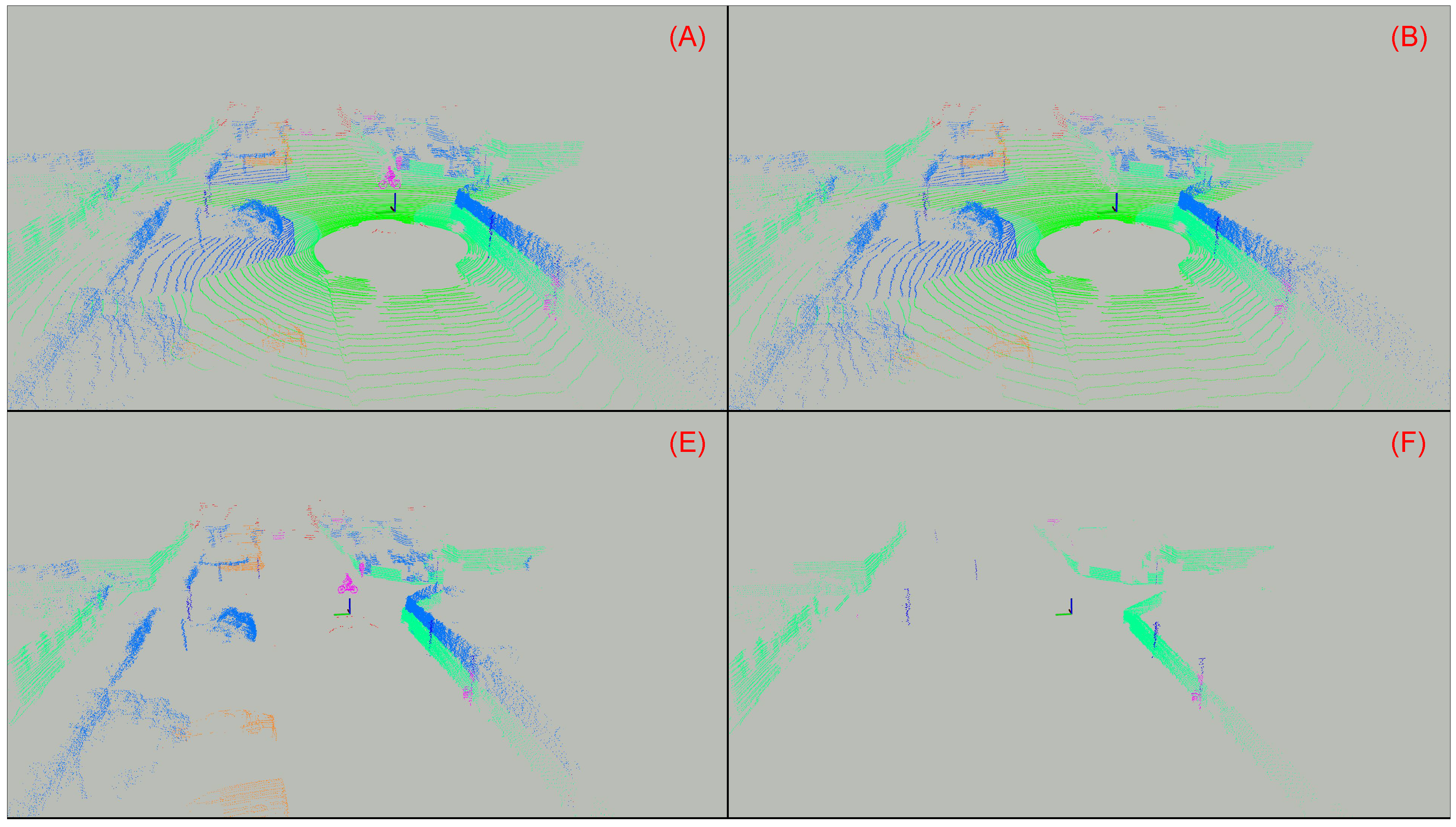
3.2. Input Configurations

To study the behavior of LiDAR odometry, six different input configurations are proposed. In each configuration, a new set of filtered data is generated, which is later fed to the odometry algorithm for evaluation. The different experimental configurations and their motivation are presented below:

(A)

Raw: Raw original point cloud from the KITTI dataset. This configuration serves as the baseline for the comparison.

(B)

Dynamic: Remove all dynamic objects from the point cloud, i.e., vehicles and pedestrians. As stated in other works (e.g., [8]), dynamic objects are a source of spurious correspondences in the matching, leading to erroneous estimations.

(C)

Dynamic Vehicles: Remove only dynamic vehicles from the point cloud. The only difference between this configuration and the previous one is that pedestrians are not removed from the point cloud. The hypothesis that motivates this configuration is that, due to their smaller size and lower velocity, the contribution of pedestrians to the error may be negligible.

(D)

Far: Remove all points that are far from the vehicle. All points p with a distance $\left|p\right|>30$ m are removed from the point cloud. This configuration is motivated by the fact that LiDAR point clouds are dense and rich in details in close distances, but become more sparse over the distance, thus far points may introduce more noise to the system.

(E)

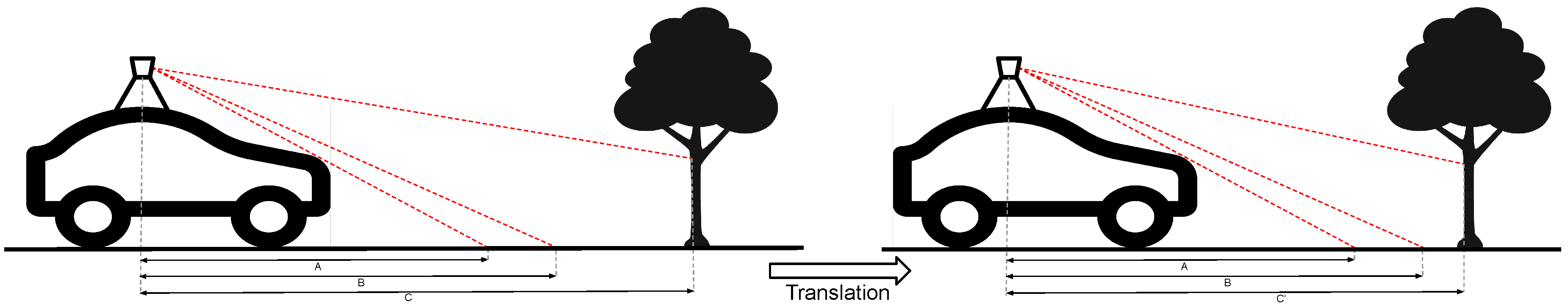
Ground: Remove the ground points. Removing the ground from the point cloud may have some advantages, but also some disadvantages. On the one hand, the rings of the LiDAR sensor that lay on the ground (assuming it is planar) will always have the same appearance. This should result in a misconceiving of the translation part because all those points will have the same coordinates in different frames, even if the vehicle was moving. On the other hand, ground points may be helpful for the rotation part, particularly for pitch and roll angles.

(F)

Structures: Leave only points from structures, such as buildings, and objects, such as poles and traffic signs. This test case is proposed to analyze what would happen if only the truly static and structured objects from the scene are kept. Everything is removed from the point cloud, including static vehicles, vegetation and the ground.

These new sequences generated after filtering the original point cloud are used as the input of the LiDAR odometry algorithm. As a result of this filtering, the total size of the point cloud is reduced. The total percentage of downsizing from the raw point cloud is visible in Figure 2, where values are averaged over all the test sequences.

3.3. Odometry Algorithm

Regarding the LiDAR odometry algorithm used in this study, we chose to evaluate LOAM [3]. The reasons to use LOAM are threefold. Firstly, it is a well-known method that has been constantly used and cited since its publication. Secondly, it ranks as the top method in the KITTI odometry leaderboard in both translation and rotation. Finally, there is an open-source implementation available [16].

LOAM algorithm divides the SLAM problem into odometry generation and map registration. These two processes run in parallel at different rates. The odometry generation algorithm runs at 10 $\mathrm{Hz}$ and computes a low fidelity motion estimation. This estimation is integrated into the registration algorithm, which runs at 1 $\mathrm{Hz}$ and optimizes the obtained odometry while building the map. To perform these computations with the point clouds, the authors proposed to extract two sets of features based on the smoothness of the points: so-called edge and planar features. Afterwards, these sets of features are processed separately, and a matching algorithm is applied to find the relative transformation between the extracted features and the map of the environment. This principle is applied by most SLAM algorithms; therefore, the collected results can be extrapolated to other LiDAR-based methods.

3.4. Evaluation Metrics

After obtaining the output odometry data for each input configuration, these estimated poses are compared with the ground-truth poses. To simplify the evaluation process, an open-source tool, evo [17], was used. This tool allows performing an insightful analysis of the generated odometry data while also providing several metrics and plotting functions.

Choosing a suitable evaluation metric has always been a subject of study. Since most LiDAR odometry algorithms are actually SLAM algorithms, we adopted two common metrics used to evaluate the estimated poses of SLAM methods. On the one hand, the Absolute Pose Error (APE) measures the absolute pose differences directly. This is computed in global coordinates and provides meaningful information about the consistency of the SLAM method because the error increases as the estimation gets farther from the reference trajectory. On the other hand, the APE metric is sensitive to errors at the beginning of the trajectory, because those early errors affect the whole estimation. For that reason, in [18], the Relative Pose Error (RPE) is proposed. This metric does not compare the poses directly; instead, it compares the measurement deltas between each pose. Therefore, RPE is more suitable for evaluating the drift of the algorithm.

Let $x_i$ and ${\widehat{x}}_i$ be the reference and estimated poses of the vehicle trajectory, respectively, where $i\in 1:T$ is the time step of each pose. Considering ⊖ the inverse of the compositional operator [19], ${\delta }_{i,j}$ is the relative transformation from pose $x_i$ to $x_j$. Accordingly, ${\widehat{\delta }}_{i,j}$ is defined as the estimated transformation from ${\widehat{x}}_i$ to ${\widehat{x}}_j$. Given this, it is possible to formulate APE and RPE metrics with (1) and (2).

$$AP{E}_i={\widehat{x}}_i\ominus x_i,\forall i\in 1:T$$

(1)

$$RP{E}_{i,j}={\widehat{\delta }}_{i,j}\ominus {\delta }_{i,j}$$

(2)

Note that, although all poses in the trajectory are considered for computing the APE metric, this is not the case for RPE. In this case, the set of pairs $\{i,j\}$ is obtained from all contiguous sub-sequences of a specific length inside the trajectory, in an analogous way as KITTI evaluation does.

Afterwards, each of the APE and RPE errors is decomposed into their translation and rotation components using (3) and (4), where $\angle \left[·\right]$ is the rotation angle [7].

$$E_{\mathrm{trans}}={\parallel E\parallel }_2$$

(3)

$$E_{\mathrm{rot}}=\angle \left[E\right]$$

(4)

4. Results and Discussion

In consideration of the extensive amount of data collected from the multiple experiments carried out, this section aims to synthesize the obtained results to provide substantial conclusions. Furthermore, the key points extracted from this analysis are presented and discussed.

4.1. Results

Table 1. Absolute Pose Error (APE) on the different KITTI odometry sequences for each configuration.

		Configuration
	Sequence	A	B	C	D	E	F
Translation ( $\mathrm{m}$)	00 (Urban)	21.8 (18.5)	21.3 (17.4)	22.1 (18.4)	41.2 (36.4)	26.8 (26.2)	36.6 (26.2)
	01 (Highway)	95.5 (69.1)	93.6 (67.9)	93.4 (67.6)	770.9 (569.1)	97.4 (71.6)	41.0 (34.4)
	02 (Urban)	142.3 (115.6)	143.3 (116.1)	142.9 (115.4)	179.4 (143.3)	91.5 (65.0)	16 656 (12 752)
	03 (Country)	4.8 (3.5)	4.7 (3.4)	4.7 (3.4)	6.2 (5.0)	3.8 (2.5)	15.8 (16.5)
	04 (Country)	2.8 (2.0)	3.0 (1.9)	3.0 (1.9)	17.1 (3.9)	2.7 (1.3)	5.4 (5.8)
	05 (Country)	12.2 (9.6)	12.1 (9.6)	12.3 (9.7)	22.2 (20.8)	10.0 (8.7)	8.6 (8.3)
	06 (Urban)	2.8 (1.9)	2.8 (1.9)	2.8 (1.7)	4.3 (1.9)	1.6 (0.8)	4.5 (6.1)
	07 (Urban)	2.8 (1.7)	2.8 (1.7)	2.8 (1.7)	4.1 (2.0)	2.5 (1.2)	7.3 (3.7)
	08 (Urban)	35.6 (30.2)	35.0 (30.0)	35.0 (30.0)	72.0 (59.3)	34.2 (29.4)	202.3 (162.2)
	09 (Urban)	15.6 (9.0)	15.3 (8.8)	15.5 (9.0)	28.6 (17.9)	17.1 (9.4)	2672 (1725)
	10 (Country)	12.9 (7.5)	12.9 (7.5)	12.9 (7.5)	12.9 (7.6)	5.5 (2.4)	141.2 (85.1)
Rotation ( ${}^{°}$)	00 (Urban)	6.0 (3.5)	5.6 (3.3)	6.2 (3.6)	11.7 (7.0)	7.8 (5.1)	11.7 (4.0)
	01 (Highway)	4.3 (1.8)	4.2 (1.6)	4.1 (1.6)	19.3 (19.6)	3.1 (1.7)	4.3 (1.6)
	02 (Urban)	31.0 (21.8)	31.2 (21.9)	31.1 (21.8)	38.2 (25.8)	19.6 (11.8)	118.9 (44.6)
	03 (Country)	1.9 (0.8)	1.9 (0.8)	1.9 (0.8)	2.5 (1.0)	1.5 (0.6)	3.7 (2.5)
	04 (Country)	0.7 (0.3)	0.8 (0.3)	0.8 (0.3)	2.9 (0.8)	0.8 (0.2)	6.3 (8.3)
	05 (Country)	3.9 (2.1)	3.9 (2.1)	3.9 (2.1)	7.5 (4.6)	3.6 (2.0)	4.4 (2.4)
	06 (Urban)	1.4 (0.6)	1.3 (0.6)	1.3 (0.6)	1.8 (0.7)	1.2 (0.6)	2.5 (1.1)
	07 (Urban)	1.7 (0.7)	1.7 (0.8)	1.7 (0.7)	2.3 (1.1)	1.8 (0.6)	4.9 (1.8)
	08 (Urban)	7.4 (4.0)	7.3 (3.9)	7.3 (4.0)	14.4 (7.2)	7.1 (3.9)	81.3 (32.7)
	09 (Urban)	3.7 (1.8)	3.6 (1.7)	3.7 (1.8)	6.9 (3.6)	4.1 (1.8)	123.0 (40.4)
	10 (Country)	2.6 (1.0)	2.6 (1.0)	2.6 (1.0)	3.2 (1.6)	1.6 (0.8)	30.3 (5.2)

and

Table 2. Relative Pose Error (RPE) on the different KITTI odometry sequences for each configuration.

		Configuration
	Sequence	A	B	C	D	E	F
Translation ( $\mathrm{m}$)	00 (Urban)	1.38 (0.87)	1.39 (0.85)	1.38 (0.85)	1.52 (0.73)	1.26 (0.79)	2.89 (1.72)
	01 (Highway)	5.93 (14.58)	5.93 (14.90)	5.97 (14.99)	430.36 (472.06)	9.83 (23.05)	1.78 (0.75)
	02 (Urban)	7.68 (22.98)	7.71 (23.05)	7.66 (22.92)	9.28 (27.71)	2.58 (5.00)	45.84 (32.42)
	03 (Country)	0.92 (0.44)	0.93 (0.45)	0.92 (0.44)	1.29 (0.49)	0.97 (0.48)	4.69 (2.41)
	04 (Country)	1.25 (0.31)	1.27 (0.31)	1.27 (0.31)	2.09 (2.26)	1.39 (0.37)	4.37 (5.13)
	05 (Country)	1.26 (0.53)	1.26 (0.54)	1.26 (0.54)	1.44 (0.59)	1.16 (0.57)	1.44 (0.80)
	06 (Urban)	1.21 (0.43)	1.21 (0.43)	1.20 (0.43)	1.41 (0.52)	1.12 (0.48)	1.36 (0.75)
	07 (Urban)	1.10 (0.59)	1.09 (0.59)	1.09 (0.59)	1.24 (0.59)	1.23 (0.68)	2.42 (1.40)
	08 (Urban)	1.48 (0.70)	1.49 (0.70)	1.49 (0.71)	1.68 (0.81)	1.34 (0.72)	4.77 (5.84)
	09 (Urban)	1.28 (0.41)	1.27 (0.42)	1.28 (0.42)	1.62 (0.55)	1.11 (0.48)	60.84 (23.32)
	10 (Country)	1.44 (0.52)	1.43 (0.52)	1.43 (0.52)	1.59 (0.48)	1.28 (0.59)	1.63 (1.36)
Rotation ( ${}^{°}$)	00 (Urban)	1.28 (0.76)	1.29 (0.76)	1.28 (0.75)	1.36 (0.68)	1.46 (0.70)	4.10 (1.85)
	01 (Highway)	0.92 (0.77)	0.89 (0.71)	0.89 (0.69)	30.77 (23.92)	0.82 (0.52)	1.05 (0.63)
	02 (Urban)	3.35 (7.18)	3.37 (7.21)	3.35 (7.18)	3.73 (7.29)	1.71 (1.80)	79.58 (54.90)
	03 (Country)	0.92 (0.34)	0.92 (0.33)	0.92 (0.33)	1.25 (0.40)	0.90 (0.35)	3.62 (2.31)
	04 (Country)	0.47 (0.25)	0.50 (0.22)	0.50 (0.22)	1.08 (0.54)	0.53 (0.28)	7.18 (8.05)
	05 (Country)	1.00 (0.58)	1.01 (0.58)	1.01 (0.58)	1.19 (0.69)	1.32 (0.65)	2.34 (0.92)
	06 (Urban)	0.87 (0.41)	0.86 (0.41)	0.86 (0.41)	1.05 (0.41)	0.87 (0.54)	1.6 (0.79)
	07 (Urban)	1.08 (0.46)	1.08 (0.46)	1.07 (0.46)	1.09 (0.48)	1.69 (0.63)	4.17 (1.30)
	08 (Urban)	1.26 (0.69)	1.26 (0.69)	1.27 (0.69)	1.50 (0.81)	1.41 (0.66)	9.50 (13.50)
	09 (Urban)	0.91 (0.52)	0.91 (0.51)	0.91 (0.52)	1.33 (0.64)	1.15 (0.59)	100.13 (54.49)
	10 (Country)	0.95 (0.59)	0.95 (0.60)	0.95 (0.60)	1.08 (0.59)	1.02 (0.57)	2.55 (3.82)

show the results obtained for APE and RPE metrics, respectively, from each odometry sequence in the KITTI dataset when applying the different proposed configurations (A–F) defined in Section 3.2. Both APE and RPE metrics are separated into translation (in meters) and rotation (in degrees). The RPE error values are obtained from all sub-sequences in the trajectory of length 100 $\mathrm{m}$. In the case of APE, the metric was computed for each pose, while in RPE it was computed for each pair of poses in each sub-sequence. For this reason, both tables show only the mean and standard deviation values, being the last one in parenthesis. Finally, the best scoring method is highlighted in bold text for each sequence and metric.

Additionally,

Table 3. Best configuration grouped for each sequence and each metric.

Sequence	Metric
	APE (Trans.)	APE (Rot.)	RPE (Trans.)	RPE (Rot.)
00 (Urban)	B (Dynamic)	B (Dynamic)	E (Ground)	A (Raw)
01 (Highway)	F (Structure)	E (Ground)	F (Structure)	E (Ground)
02 (Urban)	E (Ground)	E (Ground)	E (Ground)	E (Ground)
03 (Country)	E (Ground)	E (Ground)	C (Dyn. Vehicles)	E (Ground)
04 (Country)	E (Ground)	A (Raw)	A (Raw)	A (Raw)
05 (Country)	F (Structure)	E (Ground)	E (Ground)	A (Raw)
06 (Urban)	E (Ground)	E (Ground)	E (Ground)	C (Dyn. Vehicles)
07 (Urban)	E (Ground)	A (Raw)	C (Dyn. Vehicles)	C (Dyn. Vehicles)
08 (Urban)	E (Ground)	E (Ground)	E (Ground)	B (Dynamic)
09 (Urban)	B (Dynamic)	B (Dynamic)	E (Ground)	B (Dynamic)
10 (Country)	E (Ground)	E (Ground)	E (Ground)	B (Dynamic)

presents the best performing configurations, for each sequence and metric.

Because of the nature of the APE metric, the obtained values in Table 1 depend on the length of the sequence. Thus, it is not straightforward to combine the results obtained through all KITTI sequences. Nonetheless, since the RPE metric computes the error for each pair of poses in each subsequence of 100 $\mathrm{m}$, it is possible to better analyze the combined results of each method.

Because of the nature of the APE metric, the obtained values in Table 1 depend on the length of the sequence. This means that a larger sequence will have a larger error, due to the drift error associated to local odometry algorithms. Thus, it is not straightforward to combine the results obtained through all KITTI sequences. Nonetheless, since the RPE metric computes the error for each pair of poses in each subsequence of 100 $\mathrm{m}$, it is possible to better analyze the combined results of each method. As shown in Table 2, RPE error results are smaller as this metric measures the error along each subsequence of 100 $\mathrm{m}$. Consequently, Figure 3 contains a box-plot chart from the data obtained with the RPE metric. To generate this chart, large outliers were removed to visualize the whole data with the proper quality. In the figure, it can be observed that while Configurations A–C provide similar results (as shown in Table 1 and Table 2), the differences among the rest are more significant.

In addition to the odometry evaluation metrics, it is also of great relevance to analyze the processing time of each configuration, especially because the size of the input point clouds is reduced, which should contribute to a decrease in the processing time. Since the LOAM algorithm is implemented in different processes along different threads, we aggregated the average time of each individual process. For this reason, please note that the actual processing time is much lower, because most of the processes that were aggregated are, in fact, executed in parallel. Figure 4 shows the obtained processing times, which have a high resemblance to the point cloud sizes presented in Figure 2.

4.2. Discussion

From the deep study that was performed on the results obtained from the experiments, it is possible to extract several realizations.

First, the number of points that are reduced in the filtering step is an important factor in the odometry. As presented in Figure 2, the downsizing in configurations where dynamic vehicles are removed is very small, and the resulting size is around 99% of the original size. This is the reason the errors obtained from these configurations are very similar to the baseline. On the other hand, configurations with a heavy filter step (Ground and Structure) show more variations in the results. This is the case when we only keep structures and the point cloud is reduced up to 10% of its size. These configurations are very sensitive to the environment; therefore, environments with no structures will have several continuous frames where the odometry is completely lost. Nonetheless, these configurations also show some cases where their performance is highly superior to the baseline. A possible explanation for this is that only the most significant points are kept, while most of the noise sources are removed from the input. As a final remark, it is to be considered that smaller point clouds mean fewer points to be processed, thus reducing the computational time and allowing a higher output rate, as demonstrated with the results presented in Figure 4.

Although the disparity with the baseline is small in both downsizing and odometry error, the obtained results show a slight improvement for configurations where dynamic objects are removed. Additionally, the configuration where all dynamic objects are filtered also has better results than Configuration C, where only the dynamic vehicles are removed. This fact proves that pedestrians are also a source of noise in the odometry algorithm. As explained above, this result was expected and confirms our initial hypothesis. Nevertheless, because of the almost imperceptible change from the raw point cloud, the slight improvement that is appreciated may not be substantial enough to lead to a solid conclusion. A different dataset with a more crowded environment and a higher number of dynamic objects would be more suitable to finally consolidate this assertion.

Regarding Configuration D, which filters out all points with a distance from the sensor greater than 30 m, the obtained results quickly lead to a straightforward verdict: Even if the information in the point cloud is sparse and far from the vehicle, it is still useful for the odometry. This configuration consistently presents worse results than the baseline, which could be explained by the fact that having far references in the matching may prove helpful for the rotation computation.

Another interesting observation in the study is the variability in the results from the last configuration, where only the structures and objects are kept in the point cloud. These results are generally bad, with some noteworthy exceptions. On the one hand, because of the considerable reduction of the cloud size, the odometry algorithm encounters many areas with almost no points. This happens in roads without buildings around and with a limited number of traffic signs that could be used as references. On the other hand, this configuration works remarkably well in the highway sequence (Sequence 01). This case is of special relevance, because highway environments are the most challenging for SLAM algorithms, due to the small number of structures, the high speed of the ego-vehicle and the dynamic movement of all other vehicles. After analyzing the original point cloud, we noticed the presence of guardrails, which are labeled as “fence” and are considered structures. With only the help of these structures and traffic signs, the odometry algorithm is capable of outperforming all other methods. Furthermore, it may also appear that all points removed in this test case are prone to introduce noise to the system, as is the case for highly dynamic objects and road points, and therefore they may worsen the estimation from other configurations. Additionally, this configuration also shows adequate results in Sequence 05. This sequence also includes some kind of small walls close to the road, in a very similar way as the guardrails on the highway. We believe that having these close structures provides benefits in the matching. Nevertheless, the good results are obtained only in very specific cases, while most of the times, the algorithm gets lost because of the lack of information due to the high downsizing.

Finally, we can clearly observe in Figure 3 and Table 1 and Table 2 that removing the ground points prior to computing the odometry generally produces better results. Among the 44 test cases (including all metrics and all sequences), this configuration gives the best results in 24 of them. The only sequence that presents a problem for this configuration is Sequence 01, because of the challenging highway environment. The negative effect of ground points in the odometry algorithm is due to the uniformity of the road. When the LiDAR laser beams hit the road, they create rings of points. In a flat road, these rings will always have the same radius, which depends on the height and the characteristics of the sensor. Consequently, the points that are created always have the same coordinates, even if the vehicle is actually moving. This effect is simplified in Figure 5, where it can be observed how the distance to the object reflects the translation of the vehicle, while the distances to the points laying on the ground remain static. This absence of movement in the points may mislead the odometry algorithm into believing that there is no translation movement from the car. However, as shown in Figure 3, removing the ground points does affect the rotation error, greatly increasing the variance, while also slightly increasing the median. This leads to the conclusion that the ground points induce a negative effect in the translation component, while still being beneficial for the rotation angle. However, this configuration is the one that produces better results overall, as presented in Table 1 and Table 2.

5. Conclusions

An in-depth analysis of the use of 3D semantic knowledge to improve the performance of LiDAR odometry was carried out. The multiple experimental results confirm the effectiveness of preprocessing the raw data before feeding it to the localization algorithm. In particular, our study proved the convenience of filtering out those points belonging to dynamic objects, including pedestrians and the ground area, whereas far-off points proved useful to establish meaningful correspondences. Furthermore, it was also shown that the type of driving environment has a decisive impact on the suitability of each filtering approach. Hence, in some specific scenarios (e.g., highways), the results show that it is possible to drastically downsample the input data, thus lowering the computational requirements while improving the performance of the algorithm. This improvement is produced by reducing the occurrence of spurious correspondences in the matching process.

The analysis was performed on a very representative LiDAR SLAM approach to avoid loss of generalization; nonetheless, future work will focus on the analysis of different alternatives to further confirm the generality of the conclusions drawn from the study. Likewise, although the KITTI dataset presents a decent variety of environments, the use of additional datasets complementing its properties (e.g., featuring heavily crowded environments) is also being considered in order to strengthen some of the outcomes from the analysis. However, beyond the particularities of the study, this work serves to demonstrate that the benefits of exploiting 3D semantic information to preprocess raw LiDAR data well justify further research on this topic.

References

1. Arnold, E.; Al-Jarrah, O.Y.; Dianati, M.; Fallah, S.; Oxtoby, D.; Mouzakitis, A. A Survey on 3D Object Detection Methods for Autonomous Driving Applications. IEEE Trans. Intell. Transp. Syst. 2019, 20, 3782–3795. [Google Scholar] [CrossRef] [Green Version]
2. Behley, J.; Garbade, M.; Milioto, A.; Quenzel, J.; Behnke, S.; Stachniss, C.; Gall, J. SemanticKITTI: A Dataset for Semantic Scene Understanding of LiDAR Sequences. In Proceedings of the IEEE/CVF International Conf. on Computer Vision (ICCV), Seoul, Korea, 27 October–2 November 2019. [Google Scholar]
3. Zhang, J.; Singh, S. LOAM: Lidar Odometry and Mapping in Real-time. In Proceedings of the Robotics Science and Systems (RSS), Berkeley, CA, USA, 12–16 July 2014. [Google Scholar] [CrossRef]
4. Scaramuzza, D.; Fraundorfer, F. Visual odometry. Part I: The First 30 Years and Fundamentals. IEEE Robot. Autom. Mag. 2011, 18, 80–92. [Google Scholar] [CrossRef]
5. Sun, L.; Zhao, J.; He, X.; Ye, C. DLO: Direct LiDAR Odometry for 2.5D Outdoor Environment. In Proceedings of the IEEE Intelligent Vehicles Symposium (IV), Changshu, China, 26–30 June 2018; pp. 774–778. [Google Scholar] [CrossRef] [Green Version]
6. Yin, H.; Wang, Y.; Ding, X.; Tang, L.; Huang, S.; Xiong, R. 3D LiDAR-Based Global Localization Using Siamese Neural Network. IEEE Trans. Intell. Transp. Syst. 2019, 21, 1380–1392. [Google Scholar] [CrossRef]
7. Geiger, A.; Lenz, P.; Urtasun, R. Are we ready for Autonomous Driving? The KITTI Vision Benchmark Suite. In Proceedings of the Conference on Computer Vision and Pattern Recognition (CVPR), Providence, RI, USA, 16–21 June 2012. [Google Scholar]
8. Deschaud, J.E. IMLS-SLAM: Scan-to-Model Matching Based on 3D Data. In Proceedings of the IEEE International Conference on Robotics and Automation (ICRA), Brisbane, QLD, Australia, 21–25 May 2018; pp. 2480–2485. [Google Scholar] [CrossRef] [Green Version]
9. Zhang, J.; Singh, S. Visual-lidar Odometry and Mapping: Low-drift, Robust, and Fast. In Proceedings of the IEEE International Conference on Robotics and Automation (ICRA), Seattle, WA, USA, 26–30 May 2015; pp. 2174–2181. [Google Scholar] [CrossRef]
10. Neuhaus, F.; Koß, T.; Kohnen, R.; Paulus, D. MC2SLAM: Real-Time Inertial Lidar Odometry Using Two-Scan Motion Compensation. In Proceedings of the German Conference on Pattern Recognition 2018 (LNCS), Stuttgart, Germany, 9–12 October 2019; Volume 11269, pp. 60–72. [Google Scholar] [CrossRef]
11. Shan, T.; Englot, B. LeGO-LOAM: Lightweight and Ground-Optimized Lidar Odometry and Mapping on Variable Terrain. In Proceedings of the IEEE/RSJ International Conference on Intelligent Robots and Systems (IROS), Madrid, Spain, 1–5 October 2018; pp. 4758–4765. [Google Scholar]
12. Chen, X.; Milioto, A.; Palazzolo, E.; Giguere, P.; Behley, J.; Stachniss, C. SuMa++: Efficient LiDAR-based Semantic SLAM. In Proceedings of the IEEE/RSJ International Conference on Intelligent Robots and Systems (IROS), Macau, China, 3–8 November 2019; pp. 4530–4537. [Google Scholar]
13. Chen, S.W.; Vicentim Nardari, G.; Lee, E.S.; Qu, C.; Liu, X.; Romero, R.A.F.; Kumar, V. SLOAM: Semantic Lidar Odometry and Mapping for Forest Inventory. IEEE Robot. Autom. Lett. 2020, 5, 612–619. [Google Scholar] [CrossRef] [Green Version]
14. Li, Q.; Chen, S.; Wang, C.; Li, X.; Wen, C.; Cheng, M.; Li, J. LO-Net: Deep Real-Time Lidar Odometry. In Proceedings of the IEEE Conference on Computer Vision and Pattern Recognition (CVPR), Long Beach, CA, USA, 16–20 June 2019; pp. 8473–8482. [Google Scholar] [CrossRef] [Green Version]
15. Valente, M.; Joly, C.; De La Fortelle, A. An LSTM network for real-time odometry estimation. In Proceedings of the IEEE Intelligent Vehicles Symposium (IV), Paris, France, 9–12 June 2019; pp. 1434–1440. [Google Scholar] [CrossRef] [Green Version]
16. Laboshin, L. Open-source implementation of Laser Odometry and Mapping (LOAM). Available online: https://github.com/laboshinl/loam_velodyne (accessed on 22 July 2020).
17. Grupp, M. Evo: Python Package for the Evaluation of Odometry and SLAM. 2017. Available online: https://github.com/MichaelGrupp/evo (accessed on 22 July 2020).
18. Kümmerle, R.; Steder, B.; Dornhege, C.; Ruhnke, M.; Grisetti, G.; Stachniss, C.; Kleiner, A. On measuring the accuracy of SLAM algorithms. Auton. Robots 2009, 27, 387–407. [Google Scholar] [CrossRef] [Green Version]
19. Lu, F.; Milios, E. Globally Consistent Range Scan Alignment for Environment Mapping. Auton. Robots 1997, 4, 333–349. [Google Scholar] [CrossRef]
Figure 1. Samples of point clouds resulting from some of the tested configurations. Letters (A,B,E,F) refer to different configurations, described in Section 3.2.
Applsci 10 05657 g001
Figure 2. Point cloud downsizing with each of the tested configurations.
Applsci 10 05657 g002
Figure 3. Distribution of the RPE (in translation and rotation) across all the KITTI odometry sequences with ground truth available for each input configuration.
Applsci 10 05657 g003
Figure 4. LOAM processing time with each of the tested input configurations.
Applsci 10 05657 g004
Figure 5. Distance obtained from ground points and distance from object points after vehicle translation.
Applsci 10 05657 g005