Using Machine Learning to Grade the Mango’s Quality Based on External Features Captured by Vision System

Abstract

Nowadays, mangoes and other fruits are classified according to human perception of low productivity, which is a poor quality of classification. Therefore, in this study, we suggest a novel evaluation of internal quality focused on external features of mango as well as its weight. The results show that evaluation is more effective than using only one of the external features or weight combining an expensive nondestructive (NDT) measurement. Grading of fruits is implemented by four models of machine learning as Random Forest (RF), Linear Discriminant Analysis (LDA), Support Vector Machine (SVM), and K-Nearest Neighbors (KNN). Models have inputs such as length, width, defect, weight, and outputs being mango classifications such as grade G₁, G₂, and G₃. The unstructured data of 4983 of captured images combining with load-cell signals are transferred to structured data to generate a completed dataset including density. The data normalization and elimination of outliers (DNEO) are used to create a better dataset which prepared for machine learning algorithms. Moreover, an unbiased performance estimate for the training process carried out by the nested cross-validation (NCV) method. In the experiment, the methods of machine learning have high accurate over 87.9%, especially the model of RF gets 98.1% accuracy.

1. Introduction

Mango is a popular fruit of Asia. There has been a growing demand for high-quality mangoes in markets. Therefore, grading the quality of fruit has become vitally important for farmers. Besides, the quality of mangoes is not only affected by the growth and maturation before harvesting but also depends on the post-harvest. Manual grading and classifying of mangoes is laborious, resulting in the cost of fruits increasing and quality being uneven. Increasingly, vendors are placing requirements not only on external factors like size, color, and firmness but on internal quality factors such as sugar content and acidity. Although consumers buy fruit based on their external appearances, the taste of the fruit is used to determine whether the consumer buys again. Therefore, in this study, we use Machine Learning (ML) to grade the mango’s quality based on external features taken from the computer vision system combined with weight. The internal quality of the fruit is determined by various measurement techniques based on non-destructive testing (NDT) [1]. This technique has many advantages but it still has certain limitations such as poor reliability and the need for constant recalibration. The problem of mango evaluation has been of concern in many studies. Most of them used both numerical approach and analytical approach based on external features of mangoes such as color, dimensions, shape, weight, or defects that extracted from image data. Many authors used different algorithms of ML for evaluating the quality of mango like as a new trend in agriculture. Nandi et al. [2] proposed an ML technique for sorting mangoes in terms of maturity. The captured images from the camera are converted to the binary images and then the sizes of mangoes is estimated. These features were used to grade mango into four groups based on the Support Vector Machine (SVM) method. Pise, Dnyaneshwari, and G.D. Upadhye [3] graded mango by determining the mango’s maturity as well as quality in the form of size, shape, and surface defects. Experiments of Pandey et al. [4] considered 600 mango samples from several orchards. The quality of mango was decided by its grading standard. The classification related to distinguishing healthy or diseased mangoes, ripe or mature. Therefore, the color was used to classify fruits into different categories. Several other studies also mentioned the estimated volume of mango based on the cylinder approximation analysis method [5]. There were also some researches using both SVM and Discriminant Analysis (DA) to analyze and estimate the shape of mango. Thereby, weights of mango were determined in order to classify them [6]. The volume data were analyzed through a variety of methods. The mangoes were also classified based on their sweetness [7] which was measured with Near-Infrared Diffuse Reflectance. The quality of mangoes was also graded by maturity. Nandi et al. [8] graded the quality of mangoes based on RFE-SVM and the Multi-Attribute Decision Making (MADM) approaches. Besides, image processing was used to extract the color, size, sphericity, and weight, which was possible to know the maturity time of the mangoes in each stage as well as grading mango [9]. Procedures [2,3,4,5,6] performed well in mango classification based on weights and sizes of them. Color and defect were concerned [8,9].

In general, the combination of all the features to classify mangoes is necessary. This brings more accuracy for evaluation of mango quality. This paper proposes a novel mango grading system based on external features taken from the computer vision system combined with weight. In computer vision, a camera is used to capture the external features of mango and the weight is taken from the load-cell sensor. Furthermore, the algorithm can be applied for the other fruits. The main idea of the proposed method is to use supervised ML to grade the mango based on the combination of appearance features and density. The efficiency of the proposed method is evaluated through a small labeled dataset acquired randomly from several orchards. Supervised ML is the process based on previously labeled data to give predictions to unlabeled objects. The proposed algorithm is relevant to Multiclass Classification (MC). Many previous studies presented some effective models in fruit categorization such as Support Vector Machine (SVM) [3,5,8], Linear Discriminant Analysis (LDA) [5,6,9], Random Forest (RF) [10], and K-Nearest Neighbors (KNN) [11]. This study, by including four ML models of SVM, DA, KNN, and RF, is different from previous ones. In reality, density is directly considered as the factor of quality for a variety of fruits. The contribution of this paper is a mango classification method which uses fruit density as one of the main factors to classify quality with size and defect. Besides, density-based methods with external features can be applied to other fruits to evaluate the quality of the internal quality without complex NDT equipment. The main method based on RF algorithm is a calculation procedure using the weight and external features extracted from the vision machine. In addition, three ML models like KNN, LDA, and SVM are applied to grade and classify. On the other hand, a NCV method is employed to confirm the accuracy of mango classification. Experimental results show that the system has a high accuracy of 98.1%.

2. Structure of Quality Grading System

This study has been applied and put into practice to experiment in many orchards in Vietnam. The hardware of the grading system is shown in Figure 1. To acquire the data from captured images and evaluate geometric parameters of mangoes, several models are employed. The signal of weight is taken from the load-cell and processed to give weight shown in Figure 2. The signal from the load-cell is eliminated noise by Kalman filter.

A system in Figure 1 is designed and developed for this study. The sorting system consists of two main parts. The first part is the image processing system that implements conventional image processing using a series of algorithms that convert unstructured data into structured data to extract three external features such as length, width, and defect. The external features of mangoes can be extracted by various methods such as image processing, ML, and deep learning. In this study, the image processing is more efficient, because of its fast processing time without a large training dataset. This method changes processing parameters, which are determined more difficult in both ML and deep learning. The extracted features of the captured image are combined with weight to generate a full data set in order to leverage machine learning models. The second part is the weighting and grading system to classify mango into G₁, G₂, and G₃.

In the sorting system, the mangoes enter the vision chamber by a roller conveyor system. During movement, the mango is rotated around the roller axis and captured at different positions by a camera to accurately predict its external features. The mangoes then move into the tray conveyor to weigh and sort them based on the central processing signal. After that, in the central processing unit, the mangoes’ weight and external features are combined to generate a data set which prepared for the training in ML models. The unstructured data is converted to structured data, then it is put into models of ML to predict the grades. Last but not least, the data transmission is carried out on the server to ensure all processed data in the best.

The density depends on weight and volume which is a function of size. The change in weight and size of mangoes gradually increases with the mango’s quality. The quality parameters such as size, shape, color, total soluble solids (TSS), acidity, pH, physiological weight, juice, pulp, and moisture content are important for evaluating the external and internal qualities. They are determined by various parameters, which involve NDT techniques. However, the most important parameter is sweetness from evaluating the internal quality. The sweetness of mango depends on its density. Mango of high density has the better quality in the range of more than 1.0. The most sort after mangoes have characteristics such as bright yellow skin and sweetness. In contrast, a mango with a lower density than 1.0 is of poor quality; it could be sour because of lack of nutrients in the maturity stage. Figure 3 shows relationship between sweetness and density. Therefore, weight a factor to classify quality along with size and defect.

The operating procedure of the system is summarized in Figure 4. Input data is processed and then ML is applied to classify mango simultaneously by the central processor. The input data undergoes several image processing algorithms to achieve structured data including length, width, defects, and weight, then saves all this data to the server. At the same time, the central processor takes data from the server to train the model and then gives predictions whether the mango is G₁, G₂, or G₃.

In many references, supervised ML models were chosen to apply because these are simple and common models in the classification that have been evaluated to be effective in a number of other studies about grading fruits with artificial intelligence. These models are simple and require few operating resources thus bring an advantage in processing time for the system. ML is used to train machines to handle the data more efficiently based on algorithms and statistical models. In this study, applying ML is implemented to grade and sort the mango by learning from data. A supervised ML algorithm is used with external assistance. The input data set is divided into testing, validation, and training data. Supervised ML is the algorithm that creates a function that maps input data to the desired outputs, which are appropriate for the classification problems. The supervised machine learning algorithm learns from training datasets for classifying the mangoes into different groups based on desired standards. All algorithms learn some kind of sample from the training dataset and apply them to the testing data for classification. The four common models are discussed include RF, LDA, SVM, and KNN. The image process of sorting mango using ML is described in the schematic of Figure 3. The software of all the experiments was carried out on Python 3.6 (Python Software Foundation, Fredericksburg, VA, USA).

3. Data Preparation for Grading Process

The accuracy of the training model depends on the diversity of data. Therefore, mango data was collected and measured in several harvesting seasons in many orchards. The features are measured many times. The number of measurements is n, the average value $\overline{A}$ of feature is shown in Equation (1). The ith absolute error $\Delta A_i$ at each measurement is given Equation (2). And the average absolute error $\overline{\Delta A}$ is determined in Equation (3).

$$\overline{A}=\frac{{\displaystyle \sum _{i=1}^n{A}_i}}{n}$$

(1)

$$\Delta A_i=\left|\overline{A}-A_i\right|$$

(2)

$$\overline{\Delta A}=\frac{{\displaystyle \sum _{i=1}^n{A}_i}}{n}$$

(3)

where,$\Delta A$ means the random error. The systematic error $\Delta A^{\prime }$ was caused by the measuring instrument and the accidental error $\overline{\Delta A}$, so the absolute error is $\Delta A=\overline{\Delta A}+\Delta A^{\prime }$. So, the relative error $\delta A$ given by (4).

$$\delta A\frac{\Delta A}{\overline{A}}100\%$$

(4)

Every measurement has errors. Therefore, the accumulated error B will be generated according to the Equation (5).

$$B=F(x_i),0<i\le n$$

(5)

where i is the index number of variable in the function F. The error $\Delta B$ is shown in Equation (6).

$$\Delta B={\displaystyle \sum _{i=1}^n\Delta x_i}$$

(6)

All samples were measured and recorded. We should find the errors in each mango and determine absolute errors of their features.

4. Image Processing

In this part, the vision machine is applied to the analysis of visible imaging. This process consists of 3 steps shown in Figure 5. In the first step, the images are acquired through the roller conveyor system inside the image processing chamber which is sealed and lighted. In the second step, captured images are processed by multiple algorithms such as increase fps (frames per second), image noise filter, edge detection, and boundary tracking. In the final step, length, width, and defect are extracted to generate a dataset. A reference [5] described a threshold method. The digital images are converted into binary images, then it is processed via a sequence of morphological image processing. Each frame is handled through different algorithms including filtered noise, edge detection, and boundary trace to detect objects in the images [12]. The structure of the hardware and the vision chamber are designed based on the required productivity of the system, therefore the flow of moving mango is treated continuously during its movement.

During the movement of mango inside the vision chamber, the image of the mango is sent to a central processor consecutively. The sorting system should handle continuously for a certain time so mango’s images are acquired in real-time. The frame rate is a factor that affects the accuracy of processing. The accuracy is proportional to the increase in frame rate. Therefore, using algorithms to increase frame rate is a suitable choice. Besides, the defect is detected from captured images, therefore depth-aware video frame interpolation [13] is used to ensure the small error estimation. The new ith frame (f_i) is created from two adjacent frames (f_i−1) and (f_i+1), the value of frame rate increases to more double. The new frame is synthesized from 2 successive frames (f_i−1) and (f_i+1) by arbitrary-time flow interpolation [14]. The intermediate frame (f_i) is relied on visual flow from image ${{f}}_{(\mathrm{i}-1)\to (\mathrm{i}+1)}$ and image ${\mathrm{f}}_{(\mathrm{i}+1)\to (\mathrm{i}-1)}$ in Equations (7) and (8).

$${ \stackrel{⌢}{\mathrm{f}} }_{\mathrm{i}\to \mathrm{i}+1}={(1-\mathrm{i})}^2{\mathrm{f}}_{(\mathrm{i}-1)\to (\mathrm{i}+1)}-\mathrm{i}(1-\mathrm{i}){\mathrm{f}}_{(\mathrm{i}+1)\to (\mathrm{i}-1)}$$

(7)

$${ \stackrel{⌢}{\mathrm{f}} }_{\mathrm{i}\to \mathrm{i}-1}=-\mathrm{i}(1-\mathrm{i}){\mathrm{f}}_{(\mathrm{i}-1)\to (\mathrm{i}+1)}{+\mathrm{i}}^2(1-\mathrm{i}){\mathrm{f}}_{(\mathrm{i}+1)\to (\mathrm{i}-1)}$$

(8)

A Gaussian filter [15] is used to solve noised image, then the boundaries of the objects are detected. The Kernel matrix slides across each row and multiply by area of the image. Let μ, σ be mean, variance of Gaussian distribution, respectively. x and y are two variables of Equation (9) and $A=1/2\pi {\sigma }^2$.

$$G(x,y)=A{e}^{\frac{-{(x-{\mu }_x)}^2}{2{\sigma }_x^2}+\frac{-{(y-{\mu }_y)}^2}{2{\sigma }_y^2}}$$

(9)

After filtering the frames, the next step is to reduce the number of dimensions of the image to detect mango position. The RGB images are converted to appropriate binary image depending on the color values. Conversion from original RGB to greyscale uses NTSC method [16]. Next, conversion from grayscale to binary image based on Otsu’s method [17]. The threshold C separates pixels into two classes. The weighted sum of variances of the two classes ${\sigma }_w^2(C)$ is defined by Equation (10). The probabilities are q₁ (Equation (11)) and q₂ (Equation (12)) which are from the I bins. Variances of the two classes are ${\sigma }_1^2$ and ${\sigma }_2^2$ mean. The means μ₁ and μ₂ of probabilities q₁ and q₂ are calculated using the Equations (13) and (14), respectively.

$${\sigma }_w^2(t)=q_1(t){\sigma }_1^2+q_2(t){\sigma }_2^2$$

(10)

$$q_1(t)={\displaystyle \sum _{i=1}^{t}P(i)}$$

(11)

$$q_2(t)={\displaystyle \sum _{i=t+1}^{I}P(i)}$$

(12)

$${\mu }_1(t)=\frac{{\displaystyle \sum _{i=1}^{t}iP(i)}}{q_1(t)}$$

(13)

$${\mu }_2(t)=\frac{{\displaystyle \sum _{i=t+1}^{I}iP(i)}}{q_2(t)}$$

(14)

From Equations (11)–(14), the variance is calculated as Equations (15) and (16).

$${\sigma }_1^2(t)={\displaystyle \sum _{i=1}^t{[i-{\mu }_1(t)]}^2\frac{P(i)}{q_1(t)}}$$

(15)

$${\sigma }_2^2(t)={\displaystyle \sum _{i=t+1}^I{[i-{\mu }_2(t)]}^2\frac{P(i)}{q_2(t)}}$$

(16)

I(x,y) is the light intensity at a single pixel and INP(x,y) is the intensity of the pixel on the binary, 0 < x < Length and 0 < y < Width. The thresholding method is used to detect the color threshold. Values exceeding the threshold value are set to 1 and vice versa values inside threshold value are set to 0. The input of the method is the gray image and the threshold value.

From the binary image, the edges of the object are highlighted, then the remaining thing is to connect those points to form the boundary of the object. There are two methods of edge detection such as algebraic and geometric methods, but algebraic methods give unstable results, so it is appropriate to use geometric methods based on partial geometric differential equations. For a better understanding of the algorithms in [18], a brief description is given. A model satisfies the maximum principle and permits a rigorous mathematical analysis was used effectively. The algorithm to find the contour of objects is done by two methods of mathematics and geometry. The boundary of the object E_int are detected and interpolated into curves according to the Equation (17).

$$E_{\mathrm{int}}={\displaystyle \underset{0}{\overset{1}{\int }}(\alpha {\left|v^{\prime }(t)\right|}^2+\beta {\left|v^{″}(t)\right|}^2)}dt$$

(17)

where v(t) = (x(s), y(s)), s ∈ (0, 1), α > 0 and β > 0 are the factors that affect the elasticity and rigidity coefficients of curve.

The edges E_ext are detected based on Equation (18) with maximum curve possible ∇I(v(t)). Combining both of the above formulas, edge detection, and boundary tracking E(v,α,β,λ) are shown through Equation (19).

$$E_{ext}=-\lambda {\displaystyle \underset{0}{\overset{1}{\int }}\left|\nabla I(v(t))\right|}dt$$

(18)

$$E(v,\alpha ,\beta ,\lambda )={\displaystyle \underset{0}{\overset{1}{\int }}(\alpha {\left|v^{\prime }(t)\right|}^2+\beta {\left|v^{″}(t)\right|}^2)}dt-\lambda {\displaystyle \underset{0}{\overset{1}{\int }}\left|\nabla I(v(t))\right|}dt$$

(19)

In the above section, the image processing methods are described to extract mango size easily and quickly through a series of effective algorithms.

5. Extracting Mango External Features from Captured Images

The images were segmented with a level of 0 for the pixel area of the mango and 1 for the remaining pixel area in each frame. The next task is to calculate the area of the pixels according to the actual size. This is the step that greatly affects the accuracy of the process. With binary images, the pixel area is used to estimate actual size by Equation (20).

$$L=K{A}_{boundary}$$

(20)

Length L is the length to be estimated, A_boundary is the number of pixels and K is a ratio constant between size in pixel and the actual size. Moving objects make the distance from the camera to the objects change, therefore the proportional constants are also changed. In other words, the rate of constant changes with the distance from the camera to the object. Therefore, the K ratio factor should be appropriately estimated. With the same length at each focal distance, the number of pixels representing that length varies. Therefore, the closer to the camera is more pixels that represent for that length. That means the area of each pixel will decrease as the distance decreases. To determine the size of the mango from a binary image whose coefficient of K changes due to the motion of the mango, the scale factor from real data is estimated K ≈ F(Length). This is a linear function because as the number of pixels increases, the length also increases. So linear planning is an appropriate option. The length is L, the number of pixels in the image is A, and the values are considered on n images. The average length $\overline{L}$ is given by Equation (21).

$$\overline{L}=\frac{1}{n}{\displaystyle \sum _{i=1}^n{L}_i}$$

(21)

From Equation (19), the $\widehat{K}$ ratio factor can be found in Equation (22).

$$\widehat{K}=\frac{{\displaystyle \sum _{i=1}^n{A}_i{L}_i-n\overline{A}\overline{L}}}{{\displaystyle \sum _{i=1}^n{A}_i^2-n{\overline{A}}^2}}$$

(22)

The length $\widehat{L}=\widehat{K}{A}_{boundary}$ is estimated by $\widehat{K}$ in Equation (20). The coefficient of determination is defined in Equation (23).

$$r^2=1-\frac{{\displaystyle \sum e_i^2}}{{\displaystyle \sum L_i^2-\frac{{({\displaystyle \sum L_i})}^2}{n}}}=\frac{{\displaystyle \sum {(L-\widehat{L})}^2}}{{\displaystyle \sum L_i^2-\frac{{({\displaystyle \sum L_i})}^2}{n}}}$$

(23)

The error of K is given in Equation (24).

$$\epsilon =\frac{1}{n}{\displaystyle \sum _{i=1}^n{(L_i-(\widehat{K}A))}^2}$$

(24)

The defect of the mango is the damage on the surface caused by insects or collisions during its growth that can be scars, dark, spots, etc. The defect areas are detected by the boundaries of the rectangle (Figure 6). All defects are accumulated on the whole surface and then give the final defect level of each mango. Therefore, the areas of its disability should first be detected and zoned to be detected effectively based on the specific areas of the binary image. The disabled areas are quite small, so they should be covered by the rectangle, so the area of the disability is the area of those rectangles. The mango defects are identified by the total pixel’s area of the zero value inside the mango boundary in the binary image. Because the pixel size ratio is K, the area of each pixel is K². Where A_defect is the number of defect pixels, ($\widehat{de}$) is estimated defect; (∆de) is error of defect depending on the error (ε) of K. We can calculate the actual defect by Equation (25).

$$de=\widehat{de}+\Delta de=(K^2+2\epsilon K)A_{defect}$$

(25)

In this section, the actual dimensions of mango are estimated through the implemented algorithms. Based on a series of calculation, the size in pixel is determined to the actual size with an acceptable error. The estimation is calibrated depending on the hardware of the machine. Besides, the size of defects on the mango’s surface is calculated based on summing defective areas.

6. Estimating Volume and Density

The estimation of volume and density depends on the shape of the mango, which varies by region and country. Therefore, the shape is extracted before estimating its volume and density. The harvested mangoes from orchards are shown in Figure 7. These mango samples are measured by the vision machine and then weighted to generate the data. The prepared data for training models are structured data converted from image and weight signal. The estimation of volume and density consists of 3 steps. In the first step, length, width, and defect are extracted from the captured image by a camera. In the second step, the length, width, and defect are combined with the weight to create the completed dataset. Finally, the volume and density are predicted approximately based on length and width and then its errors are evaluated. The schematic of the preprocessing procedure for predicting the volume and density is shown in Figure 8.

The internal quality of mango is high if its density is higher than the average level. Farmers can use their experience to evaluate the internal quality by feeling the mango in their hands. The mango volume (V) has many deterministic methods such as modeling, statistical analysis based on size or weight. In this study, the volume of mangoes is calculated based on two-dimensional images because this method not only requires little resources but also has fast processing time. Since the mango has a complex shape that helps it rotate on the roller, the image processing gives images of a mango in a random orientation. In several references, there are three variables to determine the volume of mango. However, other studies [19,20] have shown that width (wi) and length (le) are related, therefore, the volume can be determined by wi and le instead of three variables. The processed images allow us to extract the values of the mango length and width. In the extraction of features, the orientations of mangoes are random with n positions presented in Figure 9a. The mango is detected by a rectangle covering them based on image processing algorithms. During the sampling process, le and wi are extracted n times at n positions. The process of detecting mangoes and extracting le and wi are given in Figure 9b. In Figure 9b, two features are determined into n value pairs (wi,le) from ith mango at n positions. Experimental results show that the method is effective in mango in Vietnam.

The collected data from images shows the volume depending on two variables as length (le), width (wi). An actual process to measure reality mango is carried out with variables like le, wi, and V in m samples of mango. The task is to predict the volume with the length and width. So, for the regression method, le and wi are independent variables and $\widehat{V}$ is a dependent variable that is calculated by Equation (26).

$$\widehat{V}=b_0+b_{1}le+b_{2}wi$$

(26)

When predicting volume, there is always an error ε. The coefficients of the variables are $b_0,b_1,b_2$. The actual volume V is calculated in Equation (27).

$$V=b_0+b_{1}le+b_{2}wi+\epsilon$$

(27)

To evaluate the accuracy of this regression expression, we need to make the sum of squared residuals as small as possible with the sum of squared residuals ΔV determined by the Equation (28).

$$\Delta V={\displaystyle \sum _{i=1}^n{\epsilon }_i^2}={\displaystyle \sum _{i=1}^n{(V_i-{\widehat{V}}_i)}^2}={\displaystyle \sum _{i=1}^n{\left(V_i-\left(b_0+b_{1}l{e}_i+b_{2}w{i}_i\right)\right)}^2}$$

(28)

The density which varies between mangoes is determined from volume and weight. The internal quality of mango is very important to grade the quality of the mango but has not been considered in previous studies of mango classification [2,3,4,5,6,7,8,9]. The density D of a mango which is given in Equation (29) is estimated by the weight (we) that get from the load-cell and the volume is predicted by le and wi.

$$D=\Delta D+\frac{we}{b_0+b_{1}le+b_{2}wi}$$

(29)

The density function is calculated based on we and V that have an error in the estimation. Therefore, the error of the density function error is a cumulative error of we and V. Therefore, the error of the density function is determined within a range of tolerances. If the cumulative error is too large, it is a bad estimate in this case. From that point of view, the weight error is ∆we, and the volumetric error is ∆V. The cumulative error ∆D is determined in Equation (30).

$$\Delta D=\Delta we+\Delta V=\frac{1}{n}{\displaystyle \sum _{i=1}^n\left(\Delta w{e}_i+\Delta V_i\right)}$$

(30)

The cumulative error ∆D is compensated for errors of calculating and estimating the density to ensure the least error in the estimates. This section ends, the volume and density that significantly affect the quality of mangoes have been estimated by a linear regression method.

7. Using Machine Learning for Grading Mangoes

The internal quality of mango is a nonlinear function of features such as length, width, defect, and weight. The quality of mango is graded based on the local standard (VietGAP) or international standards (Global GAP), which are implemented easily to classify according to each feature, but it is difficult to grade the fruits with combination of different features. The relationship of features is found in several methods such as regression, statistical, and machine learning. In this paper, ML is proposed to grade the internal quality of mango, because of its strong ability in calculating and analyzing repeated problems. The papers [2,3,4,5,6,7,8,9,10,11,12] looked particularly closely at the application of supervised ML techniques to mango classification. Hence, in this study, four supervised learning algorithms such as SVM, LDA, KNN, and RF are proposed for grading and sorting mango. The trained models are based on the sampling mango surveys in many orchards in Vietnam. In detail, the samples of mango are randomly selected, and then their types are determined (Figure 10) by evaluating standards accurately.

Dataset is generated by manually grading mango based on density (D), volume (V), and defect (de). This manual grading is carried out by agricultural experts from Vietnam. The labeled types including G₁, G₂, and G₃ of mangoes are measured by D, V, and de from four extracted features de, we, wi, and le. Instead of estimating density and volume to classify mango type, in automatic classification, four models namely RF, LDA, KNN, and SVM are trained and evaluated by the labeled dataset obtained from the manual grading. The hardware and software of the sorting system were presented in Section 2 and the grading standard is shown in

Table 1. Standard type mango.

Types	Volume Range (mL)	Length Range (cm)	Width Range (cm)	Defect (cm2)	Density (g/mL)
G3	250–400	10–12	6–8	>5	<1
G2	401–650	12.1–14	8–9	3–5	1–1.1
G1	651–800	14.1–16	9–10	0–3	>1.1

.

The dataset is divided into three parts as training, validating, and testing data. The ten-fold Nested CV (NCV) [21] was used to separate data. In the outer layer, 10% of the original data was separated for testing data to determine the performance of models. The rest of the data was used to develop a model. The rest of the 90% of the original data was used in the inner layer for the tuning of parameters. Such data are separated into training data for the model to provide a prediction or quality assessment, the validation data are to evaluate the model’s accuracy and select the best parameters of the model based on the given output objectively. This process not only provides the best performance for algorithms but also controls overfitting. The classification of mango is implemented by four steps including normalizing data, eliminating outliers, fitting models, model evaluation. During the data collection process, there are some data points outside the distribution of a statistical dataset called outliers, these points cause a significant error in the classification model. Thus, the dataset needs to be eliminated outliers to create a better new dataset. The outliers can be detected and removed based on the normalization method such as feature scaling, min-max, and z-score, etc. Depending on the purpose, one of the above methods can be used most flexible. The best method for mango data is the z-score [22] because the normalizations are based on the mean and variance of each variable. The data points are optimized in the distribution of the variables. Because of the features are on significantly different ranges, the feature with a larger scale dominates the predicted results of machine learning. By the z-score normalization, the effect of different features scales is avoided on prediction. Using z-score normalization, four features are reshaped to be between −3 and 3. Data points outside this range are eliminated from data. The effectiveness of data normalization and elimination of outliers to the performance of the four models is illustrated in the experiment section.

The supervised ML models and implementation platforms suitable for the prediction of types of mango are determined by comparing prediction accuracies. Additionally, the optimized parameters of each model to fit the data of mango are discussed. Following analysis of the data to determine the relationship of variables, models are fitted into their parameters to achieve the most effective performance. In the previous studies, several classification models demonstrate the efficiency in grading mango as SVM [3,5,8], LDA [5,6,9], RF [10], and KNN [11]. Hence, in this paper, SVM, LDA, RF, and KNN models are applied and compared to find the most accurate model in mango classification. The framework of the training process is shown in Figure 11, which includes six parts: Input, output, Random Forest (RF), K-Nearest Neighbors (KNN), Linear Discriminant Analysis (LDA), and Support Vector Machine (SVM).

Model RF: in RF model, training data consists of k subset randomly selected with replacement. Hence, the set of k subset is denoted B = {b_i: 0 < i ≤ k}, where b_i is the ith subset. The predicted label is determined by majority vote method from k decision tree in RF. In training process, RF model separates four features into nodes to lead the final decision node. Low correlation and reasonable strength of the trees are two criteria to improve the performance of RF [23]. Consulting many parameters of RF, two criteria can be achieved by the parameters such as the number of observations that are drawn for each tree (sample_size), splitting criteria in the nodes (splitting_rule), the number of trees in the forest (n_estimators), and the maximum depth of each tree (max_depth). In sample_size, decreased sampling size produces more separate trees and hence a lower correlation between the trees, which positively affects the accuracy of aggregated prediction from trees. However, the precision of individual trees decreases, as the training requires fewer observations. Therefore, Bootstrapping, which uses random samples with replacement to control the sample size of the trees. In splitting_rule, this is one of the main characterizing the RF. There are two rules, such as Gini impurity or Entropy, but Gini impurity is the better option for this analysis, as Gini can minimize misclassification and find the largest class while Entropy finds class groups that account for about 50% of data. Hence, the computing time of Gini impurity is faster than Entropy. Each tree in the forest is created by Gini impurity [24]. In the maximum depth of each tree and the number of trees in the forest, increasing max_deep and n_estimators lead to deeper trees and more trees, respectively thereby longer computation time. Nevertheless, the prediction efficiency grows up with their increase. Hence, the choice of max_deep and n_estimators can be seen as a trade-off between strength and the accuracy of the trees.

Model KNN: Let K be the number of nearest neighbors; the predicted label is aggregated from K by Large Margin Nearest Neighbor algorithm (LMNN) [25]. In KNN, the number of neighbors is the core deciding factor. The outcome is significantly influenced by the noise of a limited number of neighbors. However, a large number of neighbors have expensive computations. Therefore, the number of neighbors depends on kinds of data sets.

At the same time, KNN and RF classify three mango types, while SVM and LDA use the ‘One_vs_all’ method [26] only to grade a single classifier per class.

Model SVM: The output is classified based on three hyperplanes hp₁, hp₂, and hp₃. Because three types of mango are classified using hyperplanes generated by various kernels, the kernel function [27] is the main parameter of SVM. The kernel functions (rbf) are proposed in this study. The parameter C and γ influence the level penalty for misclassification and the complex boundary of separation, respectively. For different data sets, these parameters are different. In this study, γ and C ranged from 0.3 to 1 and 70 to 100, respectively.

Model LDA: three linear lines $h_1^{({\theta }_1)},h_2^{({\theta }_2)},h_3^{({\theta }_3)}$ are found to separate three types including G₁, G₂, G₃, …. The main factor of the LDA model is the number of returned features which reduce the features of the initial data.

In this section, four supervised learning approaches on the theory and how to apply them to the data in this paper were discussed. The advantages and disadvantages of each model are distinct. The next experiment section will provide insight into the relevance of these models to the existing data set. To evaluate the performance of models, we proposed the well-known and persuasive evaluation metrics for classification (precision, sensitivity, F-measure (F1 score), and accuracy) [28].

8. Experiments and Discussions

These experiments used 4983 mango samples harvested from November to June to meet the requirements of standards. They were measured accurately by the sorting system of the vision machine and weight. Acquired data from grading work was important and necessary to predict exact grades. The data was collected from the vision machine to get length, width, and area of the defect. This data combined the weight of each mango measured based on load-cell. The parameters of ML were determined to grade the mango quality employing input and output sets. The features of the original data set were collected by image processing and weight. Besides, their labels were classified by the manual classification system. Training and validation data from 90% of the original data were separated by using the NCV method. Besides, testing data accounted for the remaining 10% of the original data. The ML models were implemented to grade the mango quality based on its external features and weight. The models gave the results for 3 types of mangoes as good grade (G₁), medium grade (G₂), or bad grade (G₃). Besides, these models also showed the relations between the input and output with different features. The models predicted the quality based on the qualification standards automatically instead of the manual evaluation. The credibility of models was confirmed by the empirical method using the confusion matrix to evaluate the performance of models. The accuracy of the image processing part was evidenced by the experimental results in which actual and estimated values are compared. The data was measured actually in with length, width, and area of defect by Mitutoyo’s tools with an accuracy of 0.05 mm. The testing data checked the final solution in order to confirm the actual predictive work. Besides, the weight was the subset of testing set measured by electronic scales with an error of 0.01 g. Thereby, the volume (V) of the mango was determined by the overflow method with 1000 mL glass jar with accuracy 0.4 mL. Each feature of mango such as weight, width, and length was measured 10 times to calculate the expected value. From the above sections, the models are recommended to predict types of mangoes. There are four models to apply and implement such as RF, LDA, SVM, and KNN fitted by data.

The mango samples were collected to generate data set applying to the machine learning models considered in previous sections. Then, the accidental error was determined from the comparison between the actual value and the estimated one. The measurement error was smaller, so we can say that this data is reliable and considered as the prepared dataset for machine learning algorithms. Then actual sizes were determined and compared with predicted values which are extracted by the vision machine to give the bias. Besides, the grading and sorting the fruit were carried out according to the standard applied largely. The characteristics of length, width, volume, defect, and density are described in Table 1. The column of density is not the appearance in any standard for grading the mango or other tropical fruits because their grades depend on the external features without density.

The density of mango cannot be determined indirectly, therefore the density should be predicted by the volume and weight estimated by captured images and load-cell, respectively. In this study, the mangoes are graded and classified into three groups: G₁, G₂, and G₃ with the highest quality being first grade (G₁). The steps of the image processing were experimented as shown in Figure 12. The vision machine system took the data from the captured digital images of camera and used the platform to determine the parameters of mango using specific functions. The mangoes entered the vision chamber by a roller conveyor system and were captured by a camera. In each RGB image, the mango’s defect, length, and width were extracted through the image conversion stages: Calibration image, HSV image, and binary image. In Figure 13, The distributions of length, width, and volume in the dataset have a shape similar to the Gaussian function. Besides, we observed that length and width have a linear relationship to volume (V). Hence, the volume of mango is predicted from its length and width based on the prediction model of linear regression shown in Equation (31).

$$V=-1088.2+4.1le+11.7wi$$

(31)

The estimated sizes as length and width from pixels of the binary image of mango were compared with the actual ones. Additionally, the estimated values of volume by external features were different from actual volumes, which determined by the overflow method. Thus, we utilized three measures to compare the performance of the estimation features. These measures (

Table 2. The accuracy of estimated features.

Feature of Mango	MAE	RMSE	MAPE
length	0.65371	0.67623	0.00513
width	0.50863	0.51343	0.00486
defect	0.02954	0.032215	0.00813
volume	5.79612	5.95234	0.01161
density	0.01376	0.01465	0.01283

) are the mean absolute error (MAE), the root mean square error (RMSE) [29], and the mean absolute percentage error (MAPE) [30]. According to Table 2, the results show good performance. The MAPE with the maximum value of 0.01283 and the minimum value of 0.00486 are acceptable. The MAE of length, width, defect, volume, and density are 0.65371, 0.50863, 0.02954, 5.79612, and 0.01376, respectively. Five features show that there are small error distributions due to insignificant differences between RMSE and MAE.

The importance of data normalization and elimination of outliers (DNEO) in model accuracy was mentioned in Section 7. The impact of the DNEO process on model performance is therefore presented in this section. As can be seen from

Table 3. Basic statistical information on the original data.

	Weight	Length	Width	Defect
Mean	450.066963	131.422130	85.191636	5.211869
Std	89.887420	25.330647	27.233621	4.323399
Min	112.000000	15.000000	16.000000	0.060000
25%	401.167236	114.900000	74.470000	2.550000
50%	449.835599	130.500000	81.790000	4.650000
75%	499.956623	145.900000	88.650000	7.100000
Max	784.000000	298.000000	299.000000	29.000000

, four features are in very different ranges which are determined by min and max values of variables. The ranges of we, he, wi account for (112,784), (15,300), (16,300), respectively while that of defect only from (0–29) and it is the lowest scale. Although de is important as a predictor, it intrinsically influences the result less due to its smaller value. After using the DNEO process, in

Table 4. Basic statistical information on the data using data normalization and elimination of outliers (DNEO).

	Weight	Length	Width	Defect
Mean	−50.000984	0.000703	−0.000904	0.000150
Std	1.000211	0.999763	0.999931	1.000004
Min	−1.712000	−1.739000	−1.787000	−1.731000
25%	−0.872000	−0.860000	−0.861000	−0.801000
50%	−0.020000	0.008000	0.025000	−0.054000
75%	0.866000	0.866000	0.846000	0.864000
Max	1.734000	1.737000	1.703000	1.712000

, there is a significant decrease of 218 outliers in the original data. In Figure 14a, the data points beyond the smallest, and the largest observation is considered outliers. Hence, there are a lot of outliers to remove in this data. Figure 14b indicates that the range of features is normalized to about (−1712, 1737). The effect of data normalization and elimination of outliers (DNEO) on the accuracy of the models is shown in Figure 15.

The performances of models are evaluated by using the confusion matrix because it observes the relations between the classifier outputs and the true ones. The elements in the diagonal (n_ij, i = j) (i is row identifier and j is the column identifier) are the elements correctly classified, while the elements out of the diagonal are misclassified. Four models are built with two choices: Without DNEO and with DNEO. Figure 15 shows the effect of the data normalization and elimination of outliers on four models relying on the confusion matrix. A significant increase in performance is shown in all four models, if the DNEO is used. In the original dataset, the accuracy of RF, LDA, KNN, and SVM models account for 41.31%, 44.00%, 41.31%, and 44.28%, respectively. After using DNEO, the corresponding performances of these models considerably grow up to 91.50%, 86.56%, 86.20%, and 81.90%. According to Figure 15, the accuracy of the RF model is the highest, the SVM model is the lowest.

Additionally, the prediction for class G₂ in all models is lower in the two other classes. After the implementation of the DNEO, result has unqualified performance because of uncontrolled overfitting. Additionally, models’ parameters have still not been identified optimally. Varma and Simon [21] showed that overly optimistic performance estimates can be produced by using the same data to validate and train models. They also suggested the unbiased performance estimates given in nested cross-validation (NCV). NCV method used to tune parameters with an internal NCV loop while an external NCV was used to calculate an estimate of the error. Considering the accuracy of the models by the size of the training data to select the number of folds in the NCV method (Figure 16). The horizontal axis denotes the percentage of the initial data used for training models. The vertical axis denotes the accuracy of the models that match the horizontal axis values. In Figure 16, when training about 80% of the original dataset, the accuracy of models is the highest. Therefore, in both the inner and outer loops of the NCV method, 10 folds were used to ensure that 80% of the data was used in training models.

The performance of the models was determined by testing data divided 10 times in the outer layer. The estimation of accuracy (Figure 17) was implemented 10 times corresponding to 10 folds in the outer layer. The performances of four models with adjusting their parameters were evaluated by validation and testing data. The horizontal axis denotes the evaluating iteration of model performance and the vertical axis denotes the percentage of model performance. The black line in the figure presents the training score and the red line denotes the validation score of models with the best parameters. The training and validation scores were determined by validation and testing data, respectively. Finally, the gray area around the red line shows the standard deviation in the outer layer performance of each fold.

The model’s performances show that parameter selection in the NCV method is important for controlling overfitting. The separation of the initial data into training and testing data gives a smaller effect. The accuracy of RF, LDA, KNN, and SVM increase significantly to 98.1%, 87.2%, 94.8%, and 92.7%, respectively. The RF model obtains the highest accuracy at 98.1% if (n_estimators) is range from 80 to 100 and the nodes are expanded until all leaves are pure. The accuracy of the SVM model using Kernel function (rbf) is up 92.7% with γ and C ranged from 0.3 to 1 and 70 to 100, respectively. Moreover, the KNN model has a high accuracy of 94.8% in the number of neighbors ranging from 30 to 60. Finally, when reducing the number of features returned to 1, the LDA model allocates 89.6% accuracy.

The relationship of the features is the linear or nonlinear relationships shown in Figure 18. Therefore, we should not apply the linear model to grade of mango. The data is divided into 3 parts including training data, validation data, testing data. The samples divided into three parts with 3194 training data visualized in Figure 19, remaining data includes 771 validation, and 1035 testing. The distributing data on the boundary clusters obviously. The clusters in the middle of the data field are complex to classify. Besides, the area of density (0,0.67) and (1.03,1.2) are obvious, it is difficult to determine the boundary of the remaining area of density (0.67,1.03). Because the area of density is small or large, it is easy to identify the type of mango. Meanwhile, the mango classification of the region (0.75,1.03) is difficult to decide the types of mango, because these types depend on other grading factors as weight and volume.

In the experiments, we used four models for grading and classifying. The first model LDA was applied to grade the mangoes and it gave a relative accuracy of 87.9% shown in Figure 20. The mangoes were clustered well with the density’s areas (0,0.67), and (1.03,1.2), where the mangoes are graded exactly. However, the error increased in the region of density (0.67,1.03), because the types of mangoes G₁, G₂, and G₃ have complex distribution in this density area. Thus, a significant difficulty of classification was seen in the created boundary by linear lines of the LDA method. Besides, many mangoes were classified inexactly in the area of density (0.67,1.03), which is the intersection between quality types of mangoes.

The second model SVM is similar to LDA: The clusters of mangoes have boundaries of the hyperplanes. The results of grade based on SVM have an accuracy of 92.7%. The accuracy of the model SVM depends on the Kernel function. The types of kernel functions considered for this study include linear, polynomial, rbf, and sigmoid. The experiments indicate that rbf is the most efficient Kernel function. The results show that the classification of SVM is better than the LDA model (Figure 21).

Similarly, grading results evaluation in field of density (0,0.67), and (1.03,1.2) is exact. The classification results in the density (0.67,1.03) also give more accurate results than the model of LDA, because this area is clustered by the hyperplanes, and it makes the classification more flexible. The classification based on the SVM model is reliable. However, there are inexact grades for classifying, because intersections of types blend together. Another model can support to solve inexact classification being KNN. It is an algorithm that works and is considered based on predicted points, which affect the classification results and accuracy. The accuracy of the prediction is the proportion inversely neighbors of predicted points. If the number of neighbors are 30, the KNN model gives grading results shown in Figure 22.

The classification in density area (0.67,1.03) had more improvement than the SVM model, but in the remaining area, the KNN model is less reliable than the SVM model, because the boundaries of areas are distinct. Therefore, KNN is suitable for problems having many intersections. Three methods LDA, SVM, and KNN have their own advantages as well as a disadvantage in classifying mangoes or fruits.

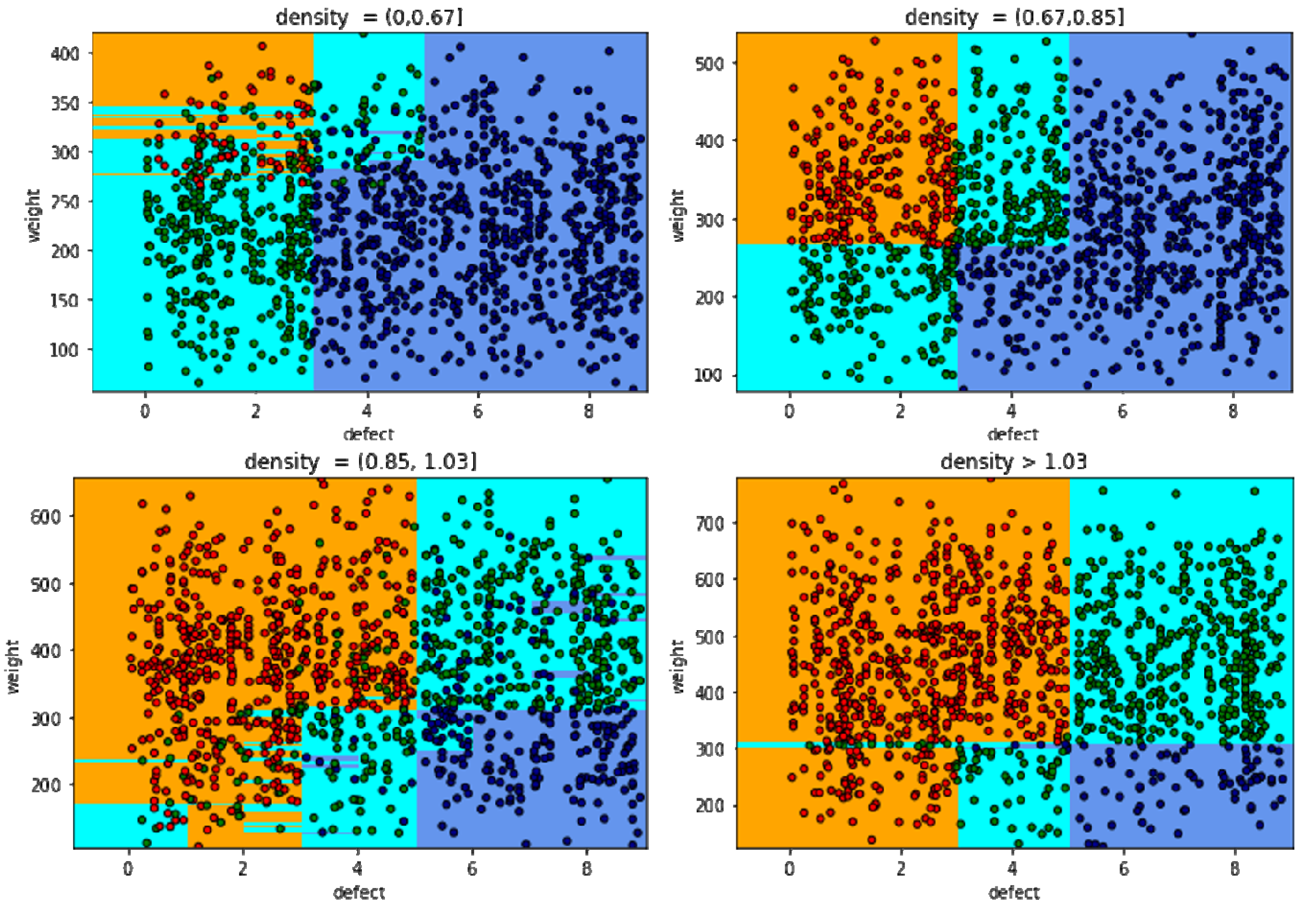
The final model of RF overcome the disadvantages of previous models. This model has differing accuracy depending on the number of trees in the forest. If the number of trees increases in number from 80 to 100 trees, the accuracy of the RF model is between 97 to 98.1%. Therefore, the selected parameters for RF model is to ensure the stability and training speed of the number of trees (Figure 23). The disadvantages of the previous models are solved in the area of (0,12) explicitly and accurately according to the rules. The accuracy depends on the complex boundaries between types of mango. From experimental performances of four models LDA, SVM, KNN, and RF, the RF model is selected to grade mangoes’ quality. Figure 24 shows the comparison and evaluation of grading results based on four models to give the best model. Besides,

Table 5. The accuracy of model.

Type		G1	G2	G3	Sensitivity (%)	Precision (%)	F1 Score (%)	Accuracy (%)
Random Forest	G1	348	2	0	99.4	98.6	99.0	98.1
	G2	5	305	7	96.2	97.8	97.0
	G3	0	5	361	98.6	97.6	98.1
Linear Discriminant Analysis (LDA)	G1	320	25	5	91.4	90.4	90.9	87.9
	G2	30	253	34	79.8	83.8	81.8
	G3	4	24	338	92.3	89.7	91.0
K-Nearest Neighbors (KNN)	G1	338	5	7	96.6	94.9	95.6
	G2	15	282	20	89.0	95.3	92.2	94.8
	G3	3	9	354	96.7	96.7	96.7
Support Vector Machine (SVM)	G1	336	7	7	96.0	93.1	94.6
	G2	24	277	16	87.4	91.1	89.3	92.7
	G3	1	20	348	94.3	93.8	94.1

shows sensitivity, precision, F1 score, and accuracy as well as the differences between models for grading [28]. All models give accuracies of more than 87.9%. The best model is RF with an accuracy of 98.1%. RF model performed best with average values of sensitivity, precision, F1 score, and accuracy of 98.1%, 98.0%, 98.0%, and 98.1%, respectively. The sensitivity and precision values show that 98.1% of three types (G₁, G₂, and G₃) were correctly classified as corresponding three types and 98.0% correctly predicted types to the total predicted corresponding types. Besides, the lowest performance is LDA model with average values of sensitivity, precision, F1 score, and accuracy of, respectively, 87.8%, 87.9%, 87.8%, and 87.9%. In comparison, the KNN model results yielded average values of sensitivity, precision, F1 score, and accuracy of, respectively, 94.1%, 95.6%, 94.5%, and 94.8%, and corresponding average values for SVM model are 92.6%, 92.0%, 92.3%, and 92.7%. F1 score (98.0%) and accuracy (98.1%) for the RF model are greater than corresponding values for the KNN, SVM, and LDA models. Overall, the results from Table 5 show that the RF model outclassed the KNN, SVM, and LDA models in predicting the types of mango in this study.

9. Conclusions

The classification was implemented with supporting the ML algorithms based on external features and weights of mangoes and then using four ML models as LDA, SVM, KNN, and RF respectively to grade mango automatically. There are several conclusions drawn as follows:

-

In this study, the quality of mango is classified by four models (RF, LDA, KNN, and SVM). The models have high accurate over 87.9%, especially the model of RF has the best predictive precision of 98.1% compared with 3 remaining models. Therefore, classification based on rules generated from input variables is suitable to classify the quality of mango.

-

Throughout the classification, a sequence of analytical methods in computer vision is used to transform the captured image of the mango to the image form that can be easily extracted feature from the mango. The experiment shows that such methods are successful when the predicted results have a small error.

-

The solution of designed ML could maintain high prediction accuracy for different mangoes. However, it should be applied similarly to the sample mangoes.

-

This study classifies mangoes based on four features consist of length, width, defect, and weight. The results showed that successful combination of extracted features as mangoes are classified with 98.1% accuracy.

-

This study indicated that data normalization and the elimination of outliers are essential to enhance the grading accuracy of mango. The results demonstrated a significant increase in the accuracy of the mango grading by over 37.5%. Furthermore, by optimizing its parameters, the performance of models increased by more than 6.5% (except for the LDA model, which only increased by 1.34%). Consequently, high accuracy is achieved not only by a good combination of the extracted features but also by the properties of machine learning.