Quantitative Evaluation of the Spatial Variation of Surface Soil Properties in a Typical Alluvial Plain of the Lower Yellow River Using Classical Statistics, Geostatistics and Single Fractal and Multifractal Methods

Featured Application

Spatial variability has always been a hot topic in soil science. Through an example of calculation, we compare and analyse the results of four methods: classical statistics, geostatistics, fractal and multifractal. Given this research scale, different methods have different conclusions. Considering that classical statistics, geostatistics and the fractal method have different disadvantages in application, we think that the multifractal method has broad prospects in the quantitative evaluation of spatial variability.

Abstract

The spatial variability of soil properties has always been a significant research field in geoscience. The types of soil properties cover a wide range, but most studies have focused on the spatial variability of soil physicochemical properties over the past decades. Studies on soil hydraulic characteristics are limited, and most of them are limited to the farmland scale. However, the spatial variability of regional soil properties (soil texture and hydraulic properties) is valuable for the study of sedimentation processes and soil water transport. Therefore, here, the spatial variation of six soil properties (sand, silt, clay content, bulk density, saturated water content and saturated hydraulic conductivity) in the typical alluvial plain area of the lower Yellow River is quantitatively studied, by using classical statistics, geostatistics and single fractal and multifractal methods. This study mainly quantitatively analysed the spatial variability of different soil properties and compared four research methods. Although the coefficient of variation, nugget coefficient, single fractal dimension and multifractal spectral width can reflect spatial variability, diverse conclusions are drawn (on variability) if different methods are used, and the different soil properties show large disparities. These four methods show a different variation order of soil properties, but there are some common conclusions based on analysis and judgment. In general, the silt content in the study area is stable, mainly originating from loess transported by Yellow River erosion, which is also reflected in the Kriging interpolation maps under the geostatistical models. The variation in bulk density and saturated water content is weak, and the spatial variability of sand and clay content is moderate. In addition, the saturated hydraulic conductivity fluctuates violently. This may be related to the differences in local topography, human activity and the content of sand and clay, each of which significantly affects the saturated hydraulic conductivity. Classical statistics has a limitation because it fails to corelate with spatial location. Due to the small sample capacity and calculation error of lag distance, the accuracy of geostatistics and single fractal dimensions needs to be improved. Multifractal spectral analysis does not need to consider the normality of data and can quantitatively represent local characteristics; therefore, its results have high reliability.

1. Introduction

The characteristics of soil particle distribution and hydraulic properties (hereafter “soil properties”) are the basis for the study of soil moisture and solute transport [1]. However, due to soil heterogeneity, soil properties vary spatially. The determination of distribution characteristics of the soil properties at a certain scale is significant for reasonable sampling and parameter prediction.

Formerly, classical statistics and geostatistics were the main methods used to study spatial variation. Geostatistics establishes the relationship between lag distance and variables through the semivariance function, which is the main means of quantitative analysis of spatial variability and the basis of Kriging interpolation. However, geostatistics is frequently limited by the sample capacity, distribution and anisotropy, which always leads to errors in practical application. With the advancement of fractal theory, the validity and potential of applying fractals to analyse soil spatial variability have been verified by early research over the past decades; they are thus an important tool with which to quantify the spatial variability and scale transformation of soil properties [2]. The combination of fractals and geostatistics can realise the quantitative characterisation of soil property spatial variation [3]; that is, the fractal dimension increases with the distribution uniformity. Researchers all over the world have calculated the fractal dimension values of various soil properties and environmental variables of different soil types. Among them, the representative studies include soil organic matter [4,5], total nitrogen [6], pH value [7], iron manganese nodules [8], and so forth. Due to different soil types, research scales and sample capacity, the fractal dimension values are also varied, but they are all in the range of 1.7~1.96. A single fractal dimension is simple and convenient, but it can only represent the holistic spatial variability of soil properties [9]. With the development of multifractal theory, the multifractal spectrum is used to quantitatively evaluate the spatial variability of soil properties. Multifractal parameters can not only reflect the spatial variation of the soil properties, but also reveal the small-scale or partial characteristics embedded in the holistic space [10]. Zeleke and Si [11], Caniego et al. [2], Eghball et al. [12] and Liu et al. [13] have analysed the spatial variability of soil properties, such as electrical conductivity, organic matter content, soil pH value, soil nitrate, soil water and salt, according to multifractal theory and obtained good results.

In recent years, the aforementioned methods have been used to study the spatial variation of soil properties such as soil particle distribution [14,15,16], bulk density [17,18], saturated hydraulic conductivity [19,20,21,22] and unsaturated hydraulic conductivity [23,24], allowing researchers to make a series of achievements. However, multifractal research is mostly limited to the farmland scale [13,25,26,27,28]. The study of multifractals when the scale increases gradually (with a sampling interval of approximately several hundred metres) are rarely reported in the literature. In addition, there is a less joint application of multiple methods and a lack of comparative study [29,30].

Yanlou township in Lankao county is in a former old channel of the Yellow River and the Yellow River flood area. Owing to the frequent sedimentary processes and human activities, the soil structure is complex and strongly changes spatially, which is typical of the alluvial plain area in the lower Yellow River area. Therefore, this study focuses on Yanlou township and comprehensively analyses the spatial variation characteristics of six soil properties in the research area by classical statistics, geostatistics and single fractal and multifractal methods. Meanwhile, the causes of the spatial distribution of soil properties were analysed according to the spatial variability. It is found that different research methods show different results and precision. We think that the multifractal method has advantages in the quantitative evaluation of spatial variability. This research can provide a reference for the study of spatial variation, whose scale extends from the field to the regional level.

2. Materials and Methods

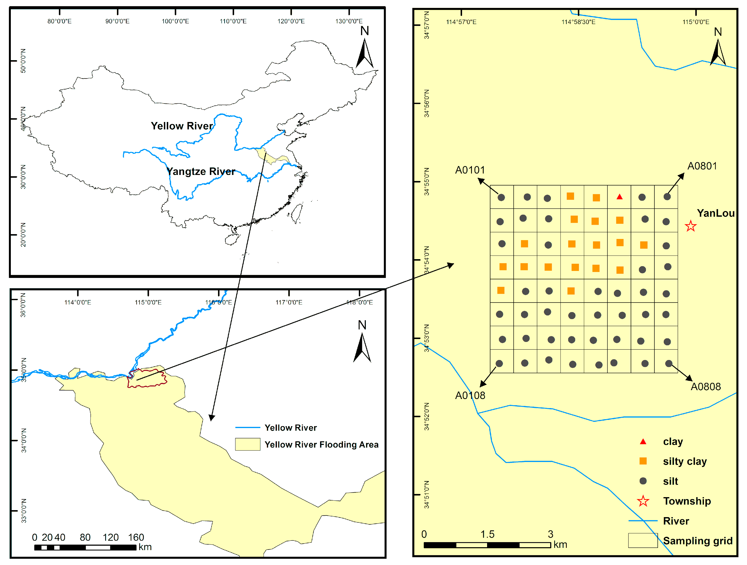
2.1. Site Description

2.1.1. Geographical Location

This study was conducted in Yanlou township, Lankao county, Henan province (114°57′23″ E~115°00′02″ E, 34°54′27″ N~34°52′31″ N), which is adjacent to the Yellow River in the northeast and is part of the lower Yellow River alluvial plain. The Quaternary Holocene strata in the study area are well-developed. Due to the repeated diversion and flooding of the Yellow River, deposits repeatedly appear, forming a large-scale alluvial fan comprising mainly loess mixed with silty fine sand and silty clay.

The study area was roughly square, with a side length of 4 km and a total area of 16 km². The terrain was relatively flat, with a maximum gradient of no more than 1.25% and a maximum height difference of 6.9 m. Most of the research areas were farmlands and villages, and the planting mode was winter wheat rotation with summer maize. The study area was divided into 64 grids with a grid cell size of 500 × 500 m.

2.1.2. Sampling and Indoor Experiment

The centre point of each grid was the coordinate of the sampling point. After the grid of the study area is surveyed and determined, a real-time kinematic (RTK) instrument is used to determine the coordinates and elevation of each grid centre. The RTK precision of this instrument is ±(8 + 1 × 10⁻⁶ × D) mm (plane precision) and ±(15 + 1 × 10⁻⁶ × D) mm (elevation precision). To ensure that the sampling point was in the grid and avoided houses and streets, the actual sampling point deviated from the centre point (Figure 1). Soil samples were taken from 20–25 cm below the surface to avoid wrapping plant roots.

Several surface soil samples were taken by ring knives, and the samples were transported to the laboratory for air drying. The division of soil particle size, the symbols and the test methods of soil properties are shown in

Table 1. Test methods of soil properties.

Soil Property	Symbol	Particle Size	Test Method
Sand	\	0.075~2mm	Sieve analysis
Silt	\	0.005~0.075mm	Densimeter method
Clay	\	<0.005mm	Densimeter method
Bulk density	γ	\	Ring knife method
Saturated water content	θs	\	Drying method
Saturated hydraulic conductivity	Ks	\	Variable head test method

. The test methods in Table 1 are strictly in accordance with the Standards for Geotechnical Testing Method (CN), GB/T50123-2019 [31]. Based on the test results, the soil texture distribution of 64 samples is shown in Figure 1. The classification of soil texture refers to the Code for Investigation of Geotechnical Engineering (CN), GB50021-2001 [32]. The coordinates of sampling points and test results can be seen in Table S1.

2.1.3. Mesh Generation

To study spatial variation by multifractal theory, it is necessary to divide the grid into different scales [13]. The study area was divided into three scales, corresponding to grids of 64, 16 and 4 (Figure 2). When the grid grew larger, the arithmetic mean value of the soil property index of the points in the cell grid was taken as the soil property index of the large grid measuring points.

2.2. Research Methods

2.2.1. Geostatistics and Fractal Method

Geostatistics is an effective method to study the spatial distribution structure characteristics of regional variables. Its basic tool is a semivariate function that can be estimated by the following formula [33]:

$$\gamma \left(h\right)=\frac{1}{2N\left(h\right)}{\displaystyle \sum _{i=1}^{N\left(h\right)}{\left[Z\left(x_i\right)-Z\left(x_i+h\right)\right]}^2}$$

(1)

where γ(h) is the variation function, Z(x) is the value of the regionalised variable at sampling point x, N(h) is the number of pairs with interval h and h is the interval, which is called the lag distance. Variograms can reflect and describe many properties of regionalised variables, and it is an important tool to analyse their spatial variation.

The fractal dimension, D, is a measure of complexity. Due to the complexity of soil structure and the local micro differences of internal soil factors, the soil property parameters are irregular and random, like random fractional Brownian motion [34]. The semivariate function in one dimension is:

$$2\gamma \left(h\right)=E\left\{{\left[Z\left(x\right)-Z\left(x+h\right)\right]}^2\right\}=h^{2H}$$

(2)

where Z(x) and Z(x + h) are the measured values at x and x + h, respectively; h is the interval (lag); and H is the power index.

For Brownian motion, the power index H is 0.5, while for the variation in soil properties, the H value ranges from 0 to 1.0. With the increase in H, the variation in soil properties gradually weaken. The fractal dimensions of these Brownian motions are given by the formula D = 2 − H.

γ(h) and h are drawn in double logarithmic space according to Formula (2). The fractal dimension D is calculated from the slope m of the regression line.

D = (4 − m)/2

(3)

The fractal dimension, D, represents the structure between samples. The smaller the value of D, the greater the difference in soil properties between samples; that is, the worse the degree of uniformity; on the contrary, the larger the value of D, the smaller the difference in soil properties between samples, and the better the degree of uniformity.

2.2.2. Multifractal Method

To further understand the role of local conditions in the formation of fractal bodies, researchers have proposed the multifractal theory that mainly discusses the probability distribution of a certain parameter. For the multifractal method, previous studies include Renyi [35] and Chhabra and Jensen [36]. The following is the calculation formula of multifractal parameters:

$${\mu }_i\left(\epsilon \right)=\frac{M_i\left(\epsilon \right)}{{\displaystyle \sum _{i=1}^{N\left(\epsilon \right)}{M}_i\left(\epsilon \right)}}$$

(4)

$$\{\begin{array}{l}D\left(q\right)=\underset{\epsilon \to 0}{\lim }\frac{1}{q-1}\frac{\lg \left[{\displaystyle \sum _{i=1}^{N\left(\epsilon \right)}{\mu }_i{\left(\epsilon \right)}^q}\right]}{\lg \epsilon }\left(q\ne 1\right)\\ D\left(q\right)=\underset{\epsilon \to 0}{\lim }\frac{{\displaystyle \sum _{i=1}^{N\left(\epsilon \right)}{\mu }_i\left(\epsilon \right)\lg {\mu }_i\left(\epsilon \right)}}{\lg \epsilon }\left(q=1\right)\end{array}$$

(5)

where μ_i(ε) is the mass probability, M_i(ε) is the variable, ε is the scale, N(ε) is the number of variables under the scale, D(q) is the generalized fractal dimension and q is the order of statistical moment.

$${\mu }_{\mathrm{i}}\left(q,\epsilon \right)=\frac{{\mu }_i{\left(\epsilon \right)}^q}{{\displaystyle \sum _{i=1}^{N\left(\epsilon \right)}{\mu }_i{\left(\epsilon \right)}^q}}$$

(6)

$$\{\begin{array}{l}\alpha \left(q\right)=\underset{\epsilon \to 0}{\lim }\frac{{\displaystyle \sum _{\mathrm{i}=1}^{N\left(\epsilon \right)}{\mu }_i\left(q,\epsilon \right)\lg {\mu }_i\left(\epsilon \right)}}{\lg \epsilon }\\ f\left[\alpha \left(q\right)\right]=\underset{\epsilon \to 0}{\lim }\frac{{\displaystyle \sum _{i=1}^{N\left(\epsilon \right)}{\mu }_i\left(q,\epsilon \right)\lg {\mu }_i\left(q,\epsilon \right)}}{\lg \epsilon }\end{array}$$

(7)

where μ_i(q, ε) is the q-order mass probability, α(q) is the singularity index and f(α) is the singularity spectrum.

q–D(q) and α–f(α) are two sets of parameters for describing multifractals. In practical application, we often use the partition function method and Legendre transformation [37] to establish the relationship between two sets of parameters:

$${\chi }_q\left(\epsilon \right)={\displaystyle \sum _{i=1}^{N\left(\epsilon \right)}{\left[{\mu }_i\left(\epsilon \right)\right]}^q}\propto {\epsilon }^{\tau \left(q\right)}$$

(8)

where χ_q(ε) is the partition function and τ(q) is the q-order mass index.

The quality index corresponding to each q value can be obtained by calculating the slope of the fitting line between log(ε) and log[χ_q(ε)] by the least-squares method. Additionally, D(q) and τ(q) have the following relationship:

D(q) = τ(q)/q − 1 q ≠ 1)

(9)

The relationship between α(q) and f[α(q)] and τ(q) is as follows:

α(q) = dτ(q)/dq

(10)

f[α(q)] = qα(q) − τ(q)

(11)

The value of q can range from negative to positive infinity. When q > 0 and D(q) decreases with q, the variable has multifractal characteristics [12]. When q >> 1, the large part of χ_q(ε) is dominant, while when q << −1, the small part of χ_q(ε) is dominant. The higher-order statistical moments can extract extreme values and enlarge their contribution. The relationship between α and f(α) can be used to analyse the local characteristics of multiple fractal bodies. The value of Δα reflects the overall heterogeneity of variable distribution; the larger the value of Δα, the greater the variability of the variable distribution. The asymmetry of the α-f(α) curve reflects the dominant power of the uneven variable distribution. If the curve is shaped like a “left hook”, the spatial variation of the variable is dominated by smaller values; on the contrary, if the curve is shaped like a “right hook”, it is dominated by the larger values.

3. Results

3.1. Classical Statistical Features

Classical statistics can directly reflect the volatility of variables. In general, the coefficient of variation (Cv) (Cv = standard deviation/mean) is used to measure the degree of variation. When 0 ≤ Cv ≤ 30%, it can be called weak variation; 30% < Cv ≤ 100% can be called medium variation; and Cv > 100% can be called strong variation. It can be seen from

Table 2. Basic statistical characteristic values of soil properties.

Soil Property	Minimum	Maximum	Mean	Standard Deviation	Cv (%)
Sand (%)	0.10	66.70	7.05	10.54	149.58
Silt (%)	33.20	95.70	81.42	10.50	12.89
Clay (%)	0.10	42.90	11.40	9.16	80.32
γ 1 (N·m−3)	12,055.20	16,056.00	14,049.35	948.95	6.75
θs 2 (cm3·cm−3)	34.47	53.24	42.53	4.00	9.41
Ks 3 (10−4cm·s−1)	0.01	28.31	4.70	5.76	122.63

¹ γ—Bulk density; ² θ_s—Saturated water content; ³ K_s—Saturated hydraulic conductivity; Cv—coefficient of variation.

that the content of silt, bulk density and saturated water content have weak variation; clay content has medium variation; and sand content and saturated hydraulic conductivity have strong variation. However, classical statistics cannot establish the relationship between variables and spatial location; therefore, geostatistics and the fractal dimension are used for further analysis.

3.2. Geostatistical Analysis

According to the Kolmogorov—Simirnov normal distribution test, the indexes of sand content, clay content and saturated hydraulic conductivity in the study area do not conform to the normal distribution, but all the six indexes follow a lognormal distribution (Table S2). To facilitate comparison, all six indexes were transformed into logarithms, which were imported into the software GS⁺9.0 for geostatistical analysis. GS9.0⁺ software allocates point pairs by establishing the lag class. When the active lag distance and lag distance interval were determined, the number of pairs was equal to the number of lag classes. Generally, the active lag distance was 80% of the maximum interval distance, 3120.86 m. Considering the distribution of sampling points, the minimum interval of 361.31 m was taken as the lag interval, and uniform distribution was selected for lag class. According to the parameter setting, there were eight pairs of points in this study. The results of isotropic analysis are shown in

Table 3. Logarithmic variogram model of soil properties in the study area.

Soil Property	Geostatistical Analysis (Isotropy)
	Model	C0 1	C0 + C 2	C0/C0 + C 3	Range(m)	R2
Sand	Gaussian	0.24450	0.49500	0.494	4094.57	0.886
Silt	Exponential	0.00001	0.00401	0.002	1119.00	0.713
Clay	Gaussian	0.10870	0.24340	0.447	5097.43	0.969
γ	Gaussian	0.00045	0.00095	0.468	1913.92	0.759
θs	Linear	0.00119	0.00185	0.402	3051.46	0.661
Ks	Spherical	0.27110	0.54320	0.499	2173.00	0.504

¹ C₀—Nugget; ² C₀+C—Sill; ³ C₀/C₀ + C—Nugget coefficient; R²—Determination coefficient.

.

The nugget is caused by random factors such as sample experimental error [38], which reflects the variation of regional variables on a small sampling scale; the sill is the half square difference of the variation function when the variable is stationary, which is the overall characteristic of the variable. The larger the sill, the stronger the spatial heterogeneity; the smaller the nugget coefficient, the stronger the spatial autocorrelation of the system; otherwise, the change between samples is closely related to random factors. The range reflects the maximum autocorrelation distance of the variable.

Table 3 reveals that there are four kinds of statistical models for the six soil properties: Gaussian, exponential, linear and spherical. The small nugget coefficient of the silt content indicates that the silt content in the study area has a strong spatial autocorrelation. Additionally, its range is the smallest, which shows that the scale range of its spatial continuity is the smallest [18]. The nugget coefficients of the other five soil properties were between 0.4 and 0.5, which can be considered to have moderate spatial autocorrelation. The order from the largest to the smallest is: K_s > sand > γ > clay > θ_s. The range values of the other five soil properties range from 1913.92 m to 5097.43 m. The sequence of the range values from the largest to the smallest is: clay > sand > θ_s > K_s > γ.

Based on the model fitted in Table 3, simple Kriging interpolation maps of soil properties (logarithm) were drawn (Figure 3), which can directly reflect the spatial distribution of soil properties. The spatial distribution of the six soil properties is varied, and there is no obvious regularity in the spatial distribution of bulk density, saturated water content and saturated hydraulic conductivity. However, two conclusions can be drawn from Figure 3: One is that the sand content gradually increases from north to south, while the clay content shows the opposite. Secondly, the colour of the silt content changes slightly, which is consistent with the extremely weak nugget coefficient of silt content, although in classical statistics, the coefficient of variation of silt content is not the lowest.

3.3. Single Fractals

The “Fractal” module (isotropy) in GS⁺9.0, with the same geostatistical parameter settings as the previous section, was used to calculate the fractal dimension, D, and determination coefficient, R², of six soil properties in the study area (

Table 4. Fractal dimension values of soil properties (isotropy).

Sand		Silt		Clay		γ		θs		Ks
D	R2	D	R2	D	R2	D	R2	D	R2	D	R2
1.832	0.817	1.932	0.590	1.786	0.972	1.838	0.767	1.899	0.572	1.944	0.478

).

According to Table 4, the fractal dimension order D is: K_s > silt > θ_s > γ > sand > clay. The fractal dimension, D, is different from the coefficient of variation, indicating that it is related to the spatial position. However, the determination coefficients of silt content, saturated water content and saturated hydraulic conductivity are less than 0.6, which led to the low accuracy.

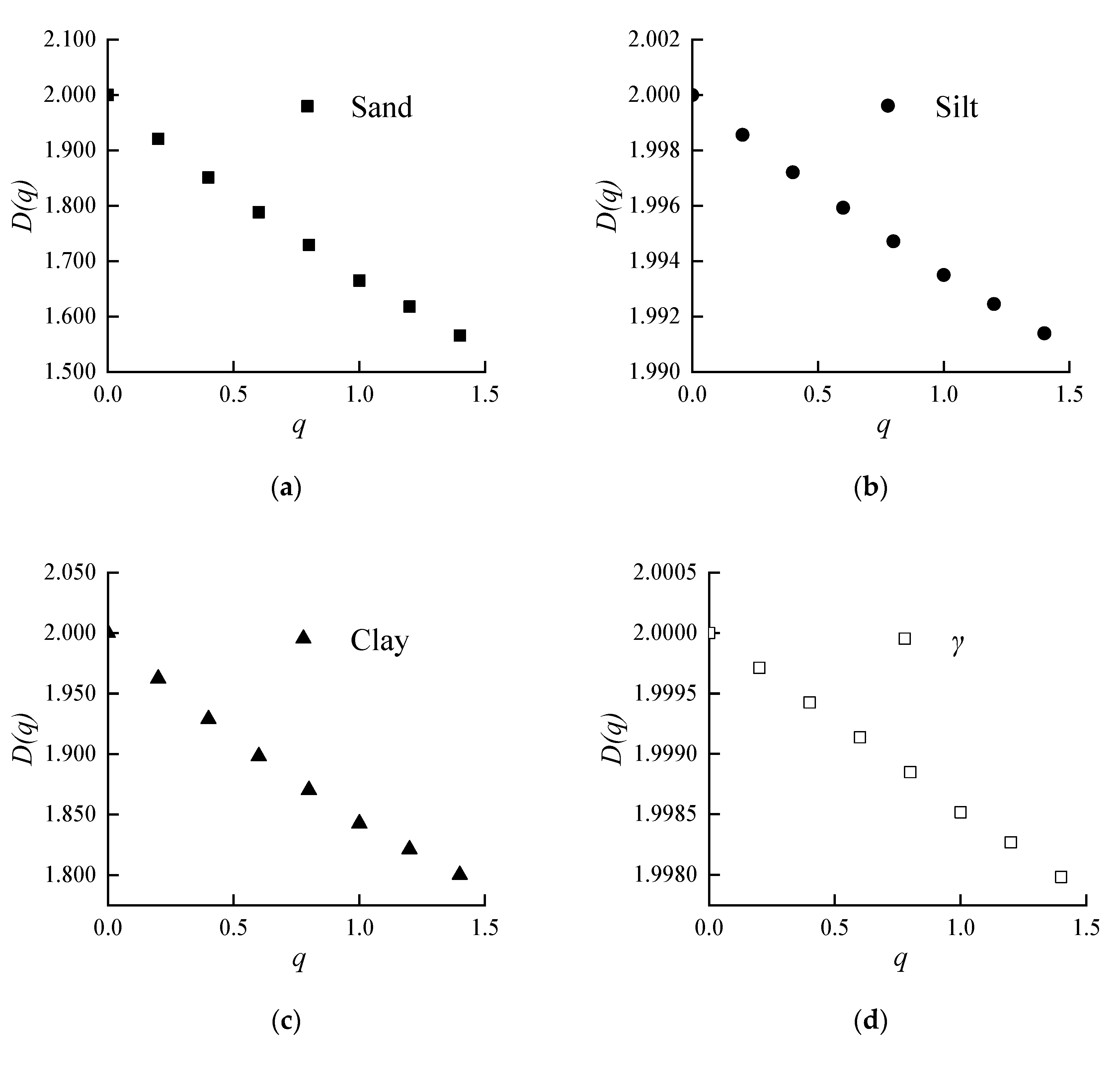
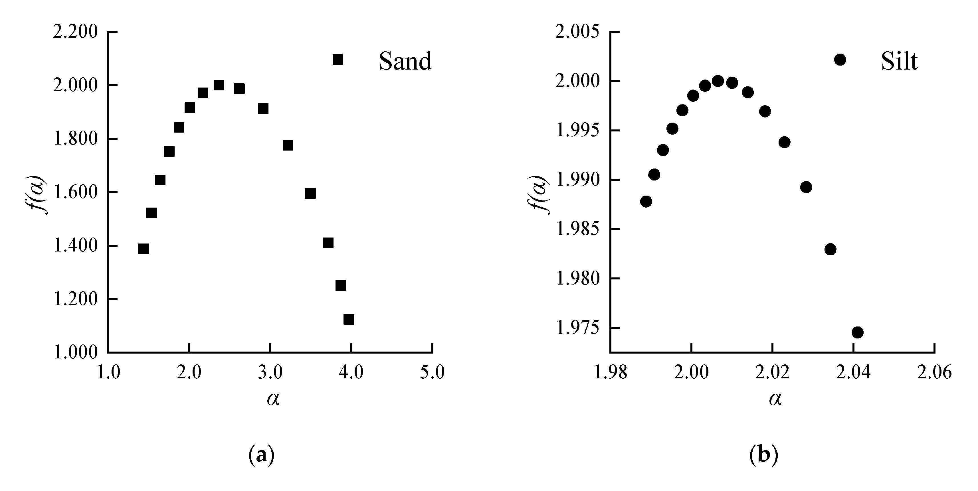
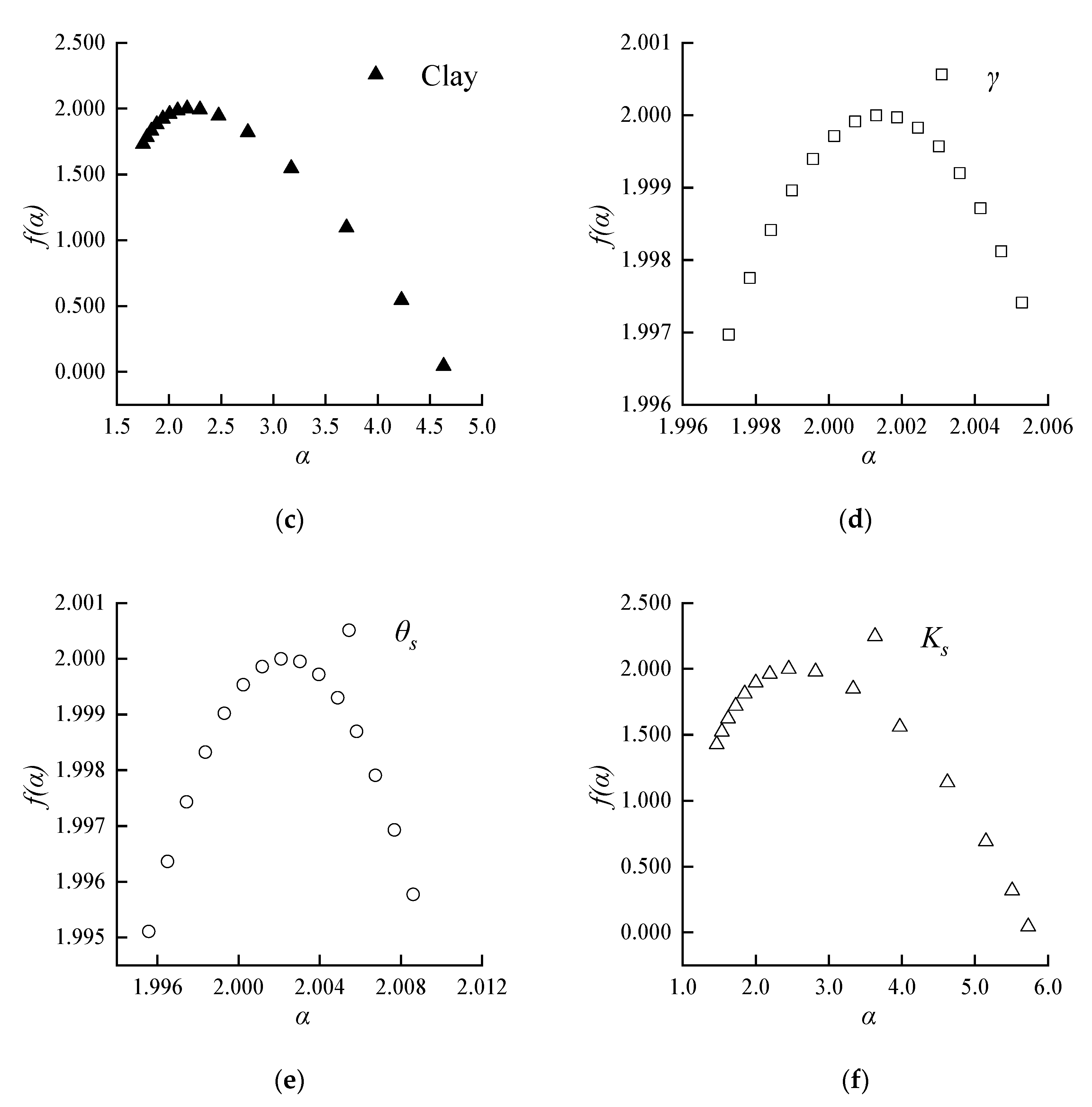
3.4. Multifractal Analysis

To determine whether the six soil properties indexes in the study area have multifractal characteristics, it was necessary to construct a q–D(q) curve for analysis (Figure 4). After debugging, q was set to −1.4 < q < 1.4, and the step size was set to 0.2. The calculation results of the multifractal parameters can be seen in Table S3.

It can be seen from Figure 4 that the D(q) of the six soil properties in the study area gradually decreases with q, and it can be determined that the six soil properties have roughly multifractal characteristics. However, the variation in D(q), that is, the generalised fractal dimension of the six soil properties, is different. The order of ΔD(q) is sand > K_s > clay > silt > θ_s > γ, which is consistent with the variation coefficient. Further analysis of the multifractal characteristics requires the multifractal spectrum, represented by the α–f(α) curve (Figure 5).

The shape of the multifractal spectrum curve can reflect the spatial distribution characteristics of the soil properties [25]. The spectral width, Δα, of the multifractal spectrum can reflect the heterogeneity of variables (

Table 5. Multifractal spectral parameters of soil properties in the study area.

Soil Properties	αmin1	f(αmin) 2	αmax3	f(αmax) 4	Δα 5	Δf 6
Sand	1.4385	1.3878	3.9716	1.1239	2.5331	0.2639
Silt	1.9888	1.9878	2.0410	1.9745	0.0522	0.0133
Clay	1.7514	1.7318	4.6308	0.0439	2.8749	1.6879
γ	1.9973	1.9970	2.0053	1.9974	0.0080	−0.0004
θs	1.9956	1.9951	2.0086	1.9958	0.0130	−0.0007
Ks	1.4648	1.4271	5.7296	0.0438	4.2648	1.3833

¹α_min—minimum value of α; ²f(α_min)—value of f(α), when α = α_min. ³ α_max—maximum value of α; ⁴ f(α_max)—value of f(α), when α = α_max. ⁵ Δα = α_max − α_min; ⁶ Δf = f(α_min) − f(α_max).

). The magnitude order of Δα of the six soil properties in the study area is K_s > clay > sand > silt > θ_s > γ. The research results of Δα, the variation coefficient and the single fractal dimension are not consistent and show that the principles of the multifractal method and geostatistics are different. The symmetry of the multifractal spectrum curve can reflect the distribution dominance of variables. According to Figure 5, the multifractal spectrum of sand, silt, clay content and saturated hydraulic conductivity is obviously “left hook”. In the process of reducing the sampling scale of these four soil properties, the large data set tends to stabilise gradually, so the spatial variation is mainly dominated by the small value data. When |q| is small, the symmetry of the multifractal spectrum curve of bulk density and saturated water content is weak, so it is necessary to define Δf[Δf = f(α_min) − f(α_max)] to determine its symmetry. The results show that the multifractal spectrum is “right hook” and the variability is dominated by large-value data (Table 5).

4. Discussion

4.1. Influencing Factors of Variability

Geostatistics shows that the distribution of silt content is stable, but the fluctuation of sand and clay content is obvious. From the perspective of structural factors, the study area is in the historical Yellow River floodplain. Its soil parent material mainly comes from fourth-century Holocene alluvial deposits, predominantly composed of silty sand. However, as the Yellow River flows through the study area, the local topographical differences result in different sedimentary separation. From the point of view of random factors, the content of clay in soil may be affected by human factors, such as farming and engineering construction, which cause variation in soil structural components.

The spatial variability of six surface soil properties in the study area is quite different, which indicates that soil properties show different development trends under the sampling interval. The soil particle distribution (sand, silt and clay content) and bulk density, as the basic physical properties of soil, largely determine the hydraulic properties of soil. The saturated hydraulic conductivity fluctuates as sharply as the content of sand and clay, which also reflects the strong effect of sand and clay on the saturated hydraulic conductivity. The variation in bulk density and saturated water content is small, and its multifractal characteristics are also weak. This is consistent with the results of Zeleke and Si [39], Guo et al. [20] and Guan et al. [25].

4.2. Comparison of Research Methods

Classical statistics can directly reflect the degree of variation of six soil properties, but it has significant limitations in analysing spatial variation. The spatial position and local characteristics of variable distribution are not considered in classical statistics, which leads to the inconsistency between the research results of the variation coefficient and geostatistics, and single and multifractal analyses. Geostatistics establishes the relationship between variable variance and lag distance, which is a powerful tool for analysing spatial autocorrelation and interpolation. The fractal dimension, D, is another important parameter in geostatistical analysis, which can quantitatively describe the exponential relationship between γ(h) and h. However, geostatistics has a large error due to the small sample capacity and lag distance calculation. For example, the geostatistical model of saturated hydraulic conductivity and the determination coefficient of the fractal value fitting line are small in this study, which led to the insufficient accuracy of the geostatistical analysis. Furthermore, the multifractal analysis considers spatial variation from another perspective, i.e., the geological process of multiple activities often produces self-similar fields, which refer to the geometric similarity maintained by the site when changing the measurement scale [40]. It establishes the relationship between the distribution of variables and the scale ε (sampling interval). It does not need the data to satisfy the normal distribution, which is a significant advantage of the multifractal analysis of spatial variation. Compared with the single fractal method, the multifractal spectrum parameters can quantitatively represent the degree of variation and help to screen the extreme value spatial distribution, which is an important indicator for local features in the region.

5. Conclusions

1.

The results of classical statistics show that the silt content, bulk density and saturated water content in the study area have weak variation; the clay content has medium variation; and the sand content and saturated hydraulic conductivity have strong variation. The variability of the six soil properties is quite different. The order of variability is sand > K_s > clay > silt > θ_s > γ, and the variation coefficient is consistent with the result of the generalised fractal dimension, ΔD(q) (q > 0).

2.

The geostatistical results (isotropy) after logarithmic transformation show that the nugget coefficient of the silt content in the study area is 0.002, so the silt content has a strong spatial autocorrelation. Its range is also the smallest, which indicates that the scale range of its spatial continuity is the smallest. The nugget coefficients of the other five kinds of soil properties are all between 0.4 and 0.5, which can be considered moderate spatial autocorrelation. The nugget coefficient can also reflect the spatial variability of soil properties to some degree, and the order from the largest to the smallest is K_s > sand > γ > clay > θ_s > silt.

3.

The single fractal (isotropy) shows that the relationship of the fractal dimension, D, is K_s > silt >θ_s > γ > sand > clay. According to the meaning of D, the larger the fractal dimension value, the smaller the variability, which shows that the variables after considering the spatial position factor (lag distance) have different statistical characteristics from the variables themselves. The fractal dimension, D, can be used as a simple and direct parameter to measure the relationship between the lag and variogram. However, due to the small sample capacity and lag distance calculation, the low accuracy leads to substantial limitations in practical application.

4.

The six soil properties in the study area have multifractal characteristics to different degrees. According to the multifractal spectrum curve, the relationship between the spectrum width, Δα, and the soil properties shows that different soil properties have different variability. The relationship order of Δα is K_s > clay > sand > silt > θ_s > γ. The symmetry of the multifractal spectrum curve can reflect the distribution dominance of variables. The content of sand, silt, clay and saturated hydraulic conductivity are obviously “left hook”, and the spatial variation is mainly dominated by small-value data. Δf values of bulk density and saturated water content are less than zero, which shows that the multifractal spectrum is “right hook”, and its variability is mainly dominated by large-value data. The multifractal method does not need to consider the normality of the data. It has higher accuracy than geostatistics and single fractal analysis and has obvious advantages in the quantitative characterisation of local characteristics and extreme values.

References

1. Gohardoust, M.R.; Sadeghi, M.; Ahmadi, M.Z.; Jones, S.B.; Tuller, M. Hydraulic conductivity of stratified unsaturated soils: Effects of random variability and layering. J. Hydrol. 2017, 546, 81–89. [Google Scholar] [CrossRef] [Green Version]
2. Caniego, F.J.; Espejo, R.; Martın, M.A.; José, S. Multifractal scaling of soil spatial variability. Ecol. Model. 2005, 182, 291–303. [Google Scholar] [CrossRef]
3. Zhang, J.; Wang, J.; Zhu, Y.; Li, B.; Wang, P. Application of fractal theory on pedology: A Review. Chin. J. Soil Sci. 2017, 48, 227–234. [Google Scholar]
4. Lv, Y.; Li, B.; Cui, Y. Micro-scale spatial variability of soil nutrients under different plant communities. Sci. Agric. Sin. 2006, 39, 1581–1588. [Google Scholar]
5. Li, X.; Zhang, S.; Wang, Z.; Zhang, H. Spatial variability and pattern analysis of soil properties in Dehui City of Jilin Province. J. Geogr. Sci. 2004, 49, 989–997. [Google Scholar]
6. Eghball, B.; Hergert, G.W.; Lesoing, G.W.; Ferguson, R.B. Fractal analysis of spatial and temporal variability. Geoderma 1999, 88, 349–362. [Google Scholar] [CrossRef]
7. Burrough, P.A. Multiscale sources of spatial variation in soil. I. The application of fractal concepts to nested levels of soil variation. Eur. J. Soil Sci. 1983, 34, 577–597. [Google Scholar] [CrossRef]
8. Blagoveschensky, Y.N.; Samsonova, V.P. Fractal and the statistical analysis of spatial distributions of Fe-Mn concretions in soddy-podsolic soils. Geoderma 1999, 88, 265–282. [Google Scholar] [CrossRef]
9. Cunha, J.M.; Campos, M.C.C.; Gaio, D.C.; Nogueira, J.S.; Soares, M.D.R.; Silva, D.M.P.; Oliveira, I.A. Fractal analysis in the description of soil particle-size distribution under different land-use patterns in Southern Amazonas State, Brazil. Afr. J. Agric. Res. 2016, 11, 2032–2042. [Google Scholar]
10. Marinho, M.A.; Pereira, M.W.M.; Vázquez, E.V.; Lado, M.; González, A.P. Depth distribution of soil organic carbon in an Oxisol under different land uses: Stratification indices and multifractal analysis. Geoderma 2017, 287, 126–134. [Google Scholar] [CrossRef]
11. Zeleke, T.B.; Si, B.C. Scaling relationships between saturated hydraulic conductivity and soil physical properties. Soil Sci. Soc. Am. J. 2005, 69, 1691–1702. [Google Scholar] [CrossRef]
12. Eghball, B.; Schepers, J.S.; Negahban, M. Spatial and temporal variability of soil nitrate and corn yield: Multifractal analysis. Agron. J. 2003, 95, 339–346. [Google Scholar]
13. Liu, J.; Ma, X.; Zhang, Z. Multifractal study on spatial variability of soil water and salt and its scale effect. Trans. Chin. Soc. Agric. Eng. 2010, 26, 81–86. [Google Scholar]
14. Brito, W.B.M.; Campos, M.C.C.; Mantovanelli, B.C.; Cunha, J.M.d.; Franciscon, U.; Soares, M.D.R. Spatial variability of soil physical properties in Archeological Dark Earths under different uses in southern Amazon. Soil Tillage Res. 2018, 182, 103–111. [Google Scholar] [CrossRef]
15. Ma, Y.; Minasny, B.; Welivitiya, W.D.P.; Malone, B.P.; Willgoose, G.R.; McBratney, A.B. The feasibility of predicting the spatial pattern of soil particle-size distribution using a pedogenesis model. Geoderma 2019, 241, 195–205. [Google Scholar] [CrossRef]
16. Zou, X.; Zhang, Z.; Wu, M.; Wan, Y. Spatial variability of particle size distribution at slope scalein Bashang region of Hebei province. Sci. Soil. Water. Conserv. 2019, 17, 44–53. [Google Scholar]
17. Qiao, J.; Zhu, Y.; Jia, J.; Huang, L.; Shao, M. Spatial variation and simulation of the bulk density in a deep profile (0–204 m) on the Loess Plateau, China. Catena 2018, 164, 88–95. [Google Scholar] [CrossRef]
18. Yu, D.; Jia, X.; Huang, L.; Shao, M.; Wang, J. Spatial variation of soil bulk density in different soil layers in the loess area and simulation. Acta Pedol. Sin. 2019, 56, 57–66. [Google Scholar]
19. Li, S.; Zhang, J.; Zhang, W.; Xiao, L. Study of spatial variability and stochastic modeling of surface soil permeability. Rock Soil Mech. 2009, 30, 300–304. [Google Scholar]
20. Guo, L.; Li, Y.; Li, M.; Ren, X.; Liu, C.; Zhu, D. Multifractal study on spatial variability of soil hydraulic properties of Lou Soil. Trans. Chin. Soc. Agric. Mach. 2011, 42, 56–64. [Google Scholar]
21. Bagarello, V.; Baiamonte, G.; Caia, C. Variability of near-surface saturated hydraulic conductivity for the clay soils of a small Sicilian basin. Geoderma 2019, 340, 133–145. [Google Scholar] [CrossRef]
22. Godoy, V.A.; Zuquette, L.V.; Gómez-Hernández, J.J. Spatial variability of hydraulic conductivity and solute transport parameters and their spatial correlations to soil properties. Geoderma 2019, 339, 59–69. [Google Scholar] [CrossRef]
23. Soto, M.A.A.; Chang, H.K.; van Genuchten, M.T. Fractal-based models for the unsaturated soil hydraulic functions. Geoderma 2017, 306, 144–151. [Google Scholar] [CrossRef] [Green Version]
24. Zhang, X.; Zhao, W.; Wang, L.; Liu, Y.; Liu, Y.; Feng, Q. Relationship between soil water content and soil particle size on typical slopes of the Loess Plateau during a drought year. Sci. Total Environ. 2019, 648, 943–954. [Google Scholar] [CrossRef] [PubMed] [Green Version]
25. Guan, X.; Yang, P.; Lv, Y. Analysis on spatial variability of soil properties based on multifractal theory. J. Basic Sci. Eng. 2011, 19, 712–720. [Google Scholar]
26. Gwenzi, W.; Hinz, C.; Holmes, K.; Phillips, I.R.; Mullins, I.J. Field-scale spatial variability of saturated hydraulic conductivity on a recently constructed artificial ecosystem. Geoderma 2011, 166, 43–56. [Google Scholar] [CrossRef]
27. Kong, D.; Wang, L.; Liu, J.; Fu, Q. Scale effect of spatial variability of cropland soil water content in black soil region. J. Hydraul. Eng. 2017, 48, 608–612. [Google Scholar]
28. Liu, J.; Zhang, S.; Ren, G.; Fu, Q.; Zhang, L.; Liu, L.; Li, J.; Yu, K.; Xu, Q. Influence of rainfall on spatial variability of soil moisture in corn farmland under straw return condition. J. Basic Sci. Eng. 2019, 27, 768–779. [Google Scholar]
29. Chen, S.; Wang, N.; Yan, F.; Zou, X. Horizontal variability and autocorrelation of soil organic matter at different soil layers inestuarine wetland. Chin. J. Ecol. 2019, 38, 2805–2812. [Google Scholar]
30. Wang, Z.; Sun, J.; Jiang, Q.; Fu, Q.; Lin, B.; He, X. Spatial distribution characteristics and influencing factors of organicmatter in black soil region of the Songnen Plain. J. Northeast. Agric. Univ. 2019, 50, 54–62. [Google Scholar]
31. General Institute of Water Resources and Hydropower Planning and Design, Ministry of Water Resources. Standards for Geotechnical Testing Method (GB/T 50123-2019); China Water&Power Press: Beijing, China, 2019. [Google Scholar]
32. Ministry of Construction of the People’s Republic of China. Code for Investigation of Geotechnical Engineering (GB5002-2001); China Architecture & Building Press: Beijing, China, 2009. [Google Scholar]
33. Journel, A.G.; Huijbregts, C.J. Mining Geostatistics; Academic Press: New York, NY, USA, 1978. [Google Scholar]
34. Burrough, P.A. Fractal dimensions of landscapes and other environmental data. Nature 1981, 294, 240–242. [Google Scholar] [CrossRef]
35. Renyi, A. Probability Theory; North-Holland: Amsterdam, The Netherlands, 1970. [Google Scholar]
36. Chhabra, A.; Jensen, R.V. Direct determination of the f(α) singularity spectrum. Phys. Rev. Lett. 1989, 62, 1327–1330. [Google Scholar] [CrossRef] [PubMed]
37. Zhou, W.; Wu, T.; Yu, Z. Geometrical characteristics of singularity spectra of multifractals II-Partition Function Definition. J. East. China Univ. Sci. Technol. 2000, 26, 62–67. [Google Scholar]
38. Zhang, N.; Zhang, D.; Qu, Z.; Lv, S.; Liu, Q. Spatial variability of soil organic matter at different sampling scales in Inner MongoliaHetao irrigation area. Chin. J. Ecol. 2016, 35, 74–84. [Google Scholar]
39. Zeleke, T.B.; Si, B.C. Characterizing scale-dependent spatial relationships between soil properties using multifractal techniques. Geoderma 2006, 134, 440–452. [Google Scholar] [CrossRef]
40. Cheng, Q. Multifractal and Geostatisic methods for characterzing local structure and singularity properities of exploration geochemical anomalies. Earth Sci. J. China Univ. Geosci. 2001, 26, 161–166. [Google Scholar]
Figure 1. Distribution of the study area and sampling points.
Applsci 10 05796 g001
Figure 2. Grid division of the study area.
Applsci 10 05796 g002
Figure 3. Kriging interpolation maps of soil properties.
Applsci 10 05796 g003
Figure 4. qD(q) curve of soil properties in the study area. q—the order of statistical moment; D(q)—the generalized fractal dimension.
Applsci 10 05796 g004aApplsci 10 05796 g004b
Figure 5. Multifractal spectrum curve of soil properties in the study area. f(α)—the singularity spectrum.
Applsci 10 05796 g005aApplsci 10 05796 g005b