Article

An Automatic Shadow Compensation Method via a New Model Combined Wallis Filter with LCC Model in High Resolution Remote Sensing Images

1
School of Geoscience, Yangtze University, Wuhan 430100, China
2
State Key Laboratory of Information Engineering in Surveying, Mapping and Remote Sensing, Wuhan University, Wuhan 430079, China
3
Institute of Geological Survey, China University of Geosciences, Wuhan 430074, China
*
Author to whom correspondence should be addressed.
Appl. Sci. 2020, 10(17), 5799; https://doi.org/10.3390/app10175799
Submission received: 13 July 2020 / Revised: 17 August 2020 / Accepted: 19 August 2020 / Published: 21 August 2020

Abstract

:
Current automatic shadow compensation methods often suffer because their contrast improvement processes are not self-adaptive and, consequently, the results they produce do not adequately represent the real objects. The study presented in this paper designed a new automatic shadow compensation framework based on improvements to the Wallis principle, which included an intensity coefficient and a stretching coefficient to enhance contrast and brightness more efficiently. An automatic parameter calculation strategy also is a part of this framework, which is based on searching for and matching similar feature points around shadow boundaries. Finally, a final compensation combination strategy combines the regional compensation with the local window compensation of the pixels in each shadow to improve the shaded information in a balanced way. All these strategies in our method work together to provide a better measurement for customizing suitable compensation depending on the condition of each region and pixel. The intensity component I also is automatically strengthened through the customized compensation model. Color correction is executed in a way that avoids the color bias caused by over-compensated component values, thereby better reflecting shaded information. Images with clouds shadows and ground objects shadows were utilized to test our method and six other state-of-the-art methods. The comparison results indicate that our method compensated for shaded information more effectively, accurately, and evenly than the other methods for customizing suitable models for each shadow and pixel with reasonable time-cost. Its brightness, contrast, and object color in shaded areas were approximately equalized with non-shaded regions to present a shadow-free image.

1. Introduction

Shadows are a common phenomenon in nature when light is occluded by objects such as buildings, clouds, and trees. In the remote sensing image acquisition process, shadows also exist in images because of low sun elevation, off-nadir viewing angles, high-rise buildings, and uneven terrain. Shadows can be categorized as cast shadows and self-shadows. A cast shadow is the part of an object that is cast on the ground, while a self-shadow is the part that is not illuminated [1]. Cast shadows were the focus of the study presented in this paper. Although objects in cast shadow areas receive some scattered sunlight from the surrounding environment, their brightness is much darker than that of the surrounding non-shaded areas. As a result, information about other objects inside cast shadows is not adequately presented, which is detrimental to extracting and reusing the shaded information. In general, this influence is positively related to the cast shadow area. The area of an object shadow is related to the object size, height, and sunlight direction, and greater shadows usually cause greater radiometric information reduction. In an image, a cloud shadow is often much larger than the shadow of a ground object [2,3]. In city construction, high-rise buildings always post larger shadows that occlude the adjacent roads and buildings. Moreover, with the development of spatial resolution of remote sensing images, this information reduction is more serious in image interpretation and affects image applications in other mapping and surveying processes. Thus, it is of great interest in the image reconstruction research arena to find a way to compensate for shaded information in remote sensing images to recover the lost information before beginning image processing steps. This compensated information can be further used in land cover classification [4], mapping, object recognition [5], etc. to improve the precision of the results.
There are two types of shadow automatic compensation methods for remote sensing image: image enhancement, compensation models. In the early 2000 s, image enhancement principles, which include Linear Correlation Correction (LCC) [6], Retinex [7,8], and histogram matching [9], were applied to shadow removal for the purpose of improving the brightness and contrast of the shadow areas in images [10,11,12,13,14]. Tsai [15] utilized the invariant color property in the shadow area to detect shadow pixels and compensated for the shaded information loss based on histogram matching. Jian Yang et al. [16] proposed an approach for global shadow compensation that utilized fully constrained linear spectral unmixing. Nair et al. [17] presented a machine-learning algorithm and an Enhanced Streaming Random Tree (ESRT) model for image segmentation and classification to extract shadow areas, after which color chromaticity and morphological processing were performed to remove shadows. Vicente et al. [18] designed a novel shadow detection and removal method based on leave-one-out optimization. First, they extracted the shadows and identified their neighboring lit regions. Next, they conducted histogram matching of the I component between the shadow regions, and the lit area was utilized to restore the shaded information. In summary, the compensation effect of their approach is related to the capability of the image enhancement algorithm and often relies on manual expertise to determine suitable parameter values. Nevertheless, it is challenging to achieve adaptive processing with this method, depending on the degree of shadow occlusion.
Thereafter, a series of compensation models based on the Gamma correction method, color constancy principle, and other methods were proposed [19,20,21]. These methods combined information from shaded areas and non-shaded areas to establish suitable compensation models. Wan et al. [22] took advantage of the Gamma correction principle to treat shadows as a multiplicative noise source. Their noise influence coefficient was related to the grayscale of the original image, and after this process, the radiation was corrected by the exponential function. Mo et al. [23] proposed an object-oriented automatic shadow detection method and a shadow compensation method by region matching based on Bag-of-Words. The I component of the shadow pixels is primarily corrected by the matched region pairs. Then, the final compensation result is heightened by the overall mean and variance of the shadow and non-shadow regions. These models generally involve many parameters; and the accuracy of the parameter values is relevant to the quality of the compensation results. However, most of the values are determined by manual expertise; and a need, therefore, exists for a way to automatically calculate suitable parameter values in shadow compensation.
All in all, the above methods cannot compensate for the information to the degree that it is the same as the non-shadow area. In addition, they are not self-adaptive enough to change the model parameters to gain the most suitable restoration, and the object’s color often deviates from the original color. Therefore, an appropriate compensation model that can improve the brightness and contrast effects similar to the non-shadow regions would be helpful. The original Wallis filter is usually used for image dodging to recover an uneven color. It typically can complement the lost color with an image contrast extension coefficient and a brightness coefficient for targeted adjusting. Yet, it cannot be used in shadow compensation directly. Since the LCC model is useful in shadow compensation, the study presented in this paper designed a compensation model based on the Wallis filter and the LCC model. Additionally, an automatic parameter calculation strategy and a final compensation combination with local information based on the designed model are discussed in detail.

2. Related Works

Most of the primary shadow compensation principles for cloud shadows and ground object shadows are similar. The image mosaic principle is often used for cloud shadow removal. However, when cloud shadows occur in high-resolution images, the typical shadow compensation methods can restore the shaded information. The shadows in high-resolution images are the primary concern of this study.
The effects of automatic shadow compensation methods depend on the capability of the compensation principles and the accuracy of the relevant parameters. Among the image enhancement principles, LCC has been shown to be more productive with fewer parameters, utilizing the target mean and variance as well as an intensity coefficient. LCC is widely used in automatic shadow compensation studies [24,25]. Chen et al. [26] used LCC to compensate for the shadow area by combining the mean and variance in the shadow and non-shadow areas with a certain compensation coefficient. The target mean and variance were obtained from the non-shadow areas; however, they applied a certain coefficient value for all the shadow regions, and their method cannot adjust based on the shadow difference. Mostafa et al. [27] detected shadows and segmented images into regions; and the shadow restoration was carried out for each region based on the degree of correspondence between the shadow and neighboring non-shadow regions and the LCC principle. Liang et al. [28] applied the LCC method to compensate for those cloud shadows which cannot be removed by image mosaic; and referring to compensation model methods, the model parameters have a vital effect on the compensation results. Zhang et al. [29] designed a cubic polynomial nonlinear compensation model and adopted the Inner-Outer Outline Profile Line (IOOPL) matching method to adaptively compensate for the shaded information. The IOOPLs were obtained for the boundary lines of shadows; and shadow removal was then performed according to the homogeneous sections through IOOPL similarity matching to provide model parameters. Friman et al. [30] implemented adaptive compensation for shadows and utilized the least-squares method to determine the parameters of the brightness correction model based on the simulated shadow cast model.
In summary, the critical principle for automatic shadow compensation is the automatic calculation of the compensation parameter value. An efficient compensation model and a reasonable parameter calculation strategy are both essential in performing accurate shadow removal. To fill this need, our method strengthened our model’s capability and designed an efficient parameter calculation strategy to improve its shadow compensation. The main highlights of our work can be summed up as follows:
(1)
By taking full advantage of Wallis filter with adjustable coefficients for contrast and brightness enhancement as well as the useful LCC model in shadow compensation, we propose a compensation model by introducing two useful intensity and stretching coefficients based on Wallis filtering and LCC model. The capability of enhancing the contrast and brightness is strengthened significantly. Then it can be applied to shadow compensation more effectively.
(2)
Customize the shadow compensation model for the pixels in each shadow region by automatic parameter calculation and a compensation combination strategy. First, the compensation parameters are calculated using automatic feature points selection and matching for each shadow area. Then, the local window information of every pixel is considered by the combination strategy. Then, the adaptive compensation model is implemented so that they are suitable to recover the shaded information more flexibly and evenly.

3. Materials and Methods

Our model compensates for the shaded information automatically in monocular true color images in Red, Green, and Blue (RGB) color space. The flow chart of our automatic shadow compensation process proceeds as follows and is also is illustrated in Figure 1. Initially, the image in RGB space is transformed into a normalized Hue, Saturation, and Intensity (HSI) color space to gather the Hue (H), Saturation (S), and Intensity (I) components. I is the only component compensated for. Then, typical shadow spectral features, such as low brightness and high normalized blue component, are employed to detect the shadows; and each shadow and non-shadow area is optimized and confirmed by their morphology. The means of the Red (R), Green (G), Blue (B) components in shadow areas and non-shadow areas are also calculated, respectively, to acquire their difference, including Δ R , Δ G , and Δ B , which are used to correct the results later in the process. The mean and standard deviation of component I of each shadow and non-shadow area are calculated. Then, the feature points around the shadow boundaries are extracted and matched to calculate the values of the unknown compensation parameters. The mean and variance of component I of each shadow and non-shadow area and the compensation parameters then are the input to build a regional improved Wallis model. Meanwhile, the mean and variance of the local window centered on each shadow pixel are calculated to establish the window compensation model. Then, the original I is heightened by combining the regional compensation with the local window compensation. In the final step, the new I, the initial H, and S are converted into RGB color space; and Δ R , Δ G , and Δ B , which represnest the difference in R, G, and B between the shadow area and non-shadow area, are subtracted from the converted R, G, B components later on so that the colors in the shadow areas are better matched with their original colors. Each step of our methodology is discussed in detail in the subsequent sections.

3.1. Shadow Detection

Before shadow compensation takes place, the shadow areas must be detected. Shadows generally have some typical spectral features such as low brightness, high hue, and high normalized blue component B′ defined in Equation (1), and low normalized green component G′ in Equation (2). These simple features cannot be combined well to detect all the shadows. Therefore, some complex signatures, such as Q defined in Equation (3), A [31] described in Equation (4) and the Morphological Shadow Index (MSI) [32,33] define in Equation (5) are applied to identify the detect condition formula for cloud shadows and ground shadows, respectively. Q and A are designed by extending the signature difference between shadow and non-shadow based on B′, I, and G′. MSI is developed based on the Differential Morphological Profiles (DMP) of black top-hat transformed data.
B = B / ( R + G + B )
G = G / ( R + G + B )
Q = B I
A = { 2 B I G ,   G T G 2 B I 2 G ,   G > T G
M S I = D M P B TH ( d , s ) D · S
where R, G, and B are red, green, and blue components in RGB space, respectively. B′ and G′ are the normalized blue component and the normalized green component, respectively. I is the intensity component in HSI space. T G is the Otsu threshold of G′. s and d indicate the length and direction of the linear structure element (SE). D M P B TH ( d , s ) is the value in DMP when using the SE(d, s). D and S denote the numbers of directionality and scale of the profiles, respectively.
Generally, the ground object shadow and cloud shadow have some similarity and difference in spectral features. For instance, the ground object shadows have larger MSI values, while the cloud shadows have smaller amounts. Then, combined with the automatic Otsu threshold strategy [34], the ground object shadow and the cloud shadow are detected using Equations (6) and (7), respectively.
C GOSD = { ( i , j ) | ( B ( i , j ) > T B & & I ( i , j ) < T I ) ( Q ( i , j ) > T Q & & G ( i , j ) < T G ) A ( i , j ) > T A M S I ( i , j ) > T M S I }
C CSD = { ( i , j ) | I ( i , j ) < T I G ( i , j ) < T G M S I ( i , j ) < T M S I }
where CGOSD and CCSD are the pixels set of ground object shadow and cloud shadow. G(i, j) represents the value of the green component in pixel (i, j). I(i, j) represents the value of intensity component I in HSI space in pixel (i, j). B′ (i, j) and G′ (i, j) represent the value of the nominalized blue and nominalized green component in pixel (i, j), respectively. Q(i, j), A(i, j), and MSI(i, j) are the corresponding value of the complex features Q, A, and MSI in pixel (i, j), respectively. T B , T I , T Q , T G , T A , T M S I , and T G , indicate the Otsu thresholds of B′, I, Q, G′, A, MSI, and G components, respectively.
Lastly, some scattered and small shadow areas are removed, and some shadow holes are filled using mathematic morphological operators such as erasing, dilating, opening, and closing. Then the final shadow regions are more complete for use in further compensation.

3.2. Shadow Compensation Model Based on Wallis Filter and LCC Model

The original Wallis filter is commonly used for image dodging to recover an uneven color. It typically can complement the lost color, but it is not sufficient enough to recover the shaded information caused by shadows. Hence, this study improved the original Wallis model by introducing the intensity coefficient and stretching coefficient to promote brightness and contrast that is more effective for shadow compensation.
The general form of the Wallis filter is defined as follows:
g c ( i , j ) = g ( i , j ) · r 1 + r 0
Or another form is expressed as follows:
g c ( i , j ) = [ g ( i , j ) m ¯ g ] ( c · σ f ) ( c · σ g + σ f c ) + b · m ¯ f + ( 1 b ) · m ¯ g
where, g c ( i , j ) and g ( i , j ) represent the target image and the original image, respectively. The parameters r 1 and r 0 are the multiplicative coefficient and the additive coefficient, respectively, where r 0 = b · m ¯ f + ( 1 b r 1 ) · m ¯ g and r 1 = ( c · σ f ) / ( c · σ g + σ f / c ) . m ¯ g and σ g represent the mean and standard deviation of the component in the local area around the pixel (i, j). m ¯ f and σ f are the target mean and standard deviation for this area, respectively. c (c∈[0,1]) is the image contrast extension coefficient, which is proportional to the local window size. b (b∈[0,1]) is the image brightness coefficient.
The original Wallis filter, essentially a type of image enhancement principle, is typically used in image dodging to solve the disproportionate color problems [35,36], but it is not functional for shadow compensation directly. For example, in Figure 2 two different types of shadows cast by a building and cloud were compensated for the component I with the original Wallis filter. Compared to the original shadow areas, the brightness after shadow compensation is strengthened slightly. However, the overall contrast and brightness in shadow areas are still not good enough to be the same as the non-shadow areas. Consequently, shaded information is not recovered completely. Its main weakness is that r 1 and r 0 are fixed when the target means and standard deviations of the features acquired from the non-shadow areas are combined with a certain b and c. Consequently, the filter is equivalent to a linear transformation. However, because the contrast and brightness in the shadow region are so low and the influence of c is not sufficient to extend the contrast, this linear transformation is not efficient enough to enlarge the difference to recover the information. When it is used for shadow compensation directly, it cannot be valid for more serious information loss by shadows. For this reason, a valid parameter to increase the contrast should be introduced to be used in shadow compensation.
Since the Linear Correlation Correction (LCC) model in Equation (10) is a very classic method and useful in shadow compensation. By using m ¯ NSD and m ¯ SD , σ NSD and σ SD , which represent the mean values and standard deviation of the Non-Shadow area (NSD) and the Shadow area (SD), this model can more accurately enhance the shadow information to the NSD value. However, it is also not able to adjust the contrast and brightness flexibly.
g c ( i , j ) = m ¯ NSD + ( g ( i , j ) m ¯ SD ) · σ NSD σ SD
Thus, in this study, a new shadow compensation model based on Wallis filter and LCC model was designed by acquiring the target value from the non-shadow area adjacent to the shadow area and adding an intensity coefficient α and a stretching coefficient β, as shown in Equation (11):
g c ( i , j ) = α · ( m ¯ NSD + g ( i , j ) m ¯ SD β · r 1 r 0 · r 1 )
where α represents the compensation intensity coefficient, β represents the stretching coefficient, m ¯ NSD and m ¯ SD represent the mean values of the Non-Shadow area (NSD) and the Shadow area (SD), r 1 and r 0 are the multiplicative coefficient and the additive coefficient in the Wallis model.
It is worth noting that this model can capture the target information from NSD areas more precisely as well as increase the average value and gradients of the shadow component more precisely. α is more useful for reinforcing the average brightness, while β is effective for enhancing the average gradient (contrast). With the help of the specific parameters, the compensation model can be more effective in heightening the information in brightness and contrast.

3.3. Automatic Parameter Calculation Method

In order to perform reasonable compensation for each shadow area, it is necessary to customize the compensation model according to their condition. Therefore, a novel method of extracting relevant regions and matching the feature points is implemented for automatically calculating the values of the compensation parameters.
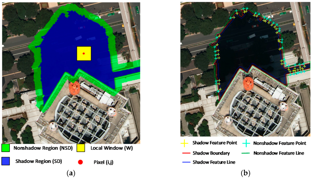
First, each shadow area and its adjacent non-shadow area as shown in Figure 3a are gained by a morphological operation to calculate m ¯ SD , m ¯ NSD , r0 and r1. The Shadow area (SD) is obtained by shadow detection initially. By applying a certain morphological dilation K1 times to each shadow area, a ring region with width K1 around each shadow area is acquired as its Non-Shadow area (NSD). The mean and standard deviation of the SD and NSD, m ¯ SD and σ SD , m ¯ NSD and σ NSD , are calculated. Additionally, combined with the empirical values of b and c, r0 and r1 are determined for each region.
Then, the feature points on the shadow and non-shadow lines are extracted and matched to automatically calculate the unknown parameters α and β . Since there are some ground objects divided by the shadow boundary into two parts, some feature points belonging to the same object can be found on both sides of the shadow boundary. As shown in Figure 3b, the non-shadow feature lines (green) and shadow feature lines (red) can be acquired by dilating and erasing the shadow region. Pairs of similar feature points are chosen by randomly selecting a series of points along the shadow boundary. Then, their closest feature points on the two types of feature lines are selected as the shadow feature point PSD and the non-shadow feature point PNSD. If they are both exposed to the same amount of sunlight, they should have similar feature values. Therefore, the feature value g c of a non-shadow feature point can be the approximate target value of its shadow similar feature value. α and β can be calculated using Equations (12) and (13) Via using similar feature point pairs, corresponding equations based on them can be constructed to estimate the unknown parameters α and β using the least-squares rule.
α = g c m ¯ NSD + ( g m ¯ SD ) · σ NSD σ SD
β = g m ¯ SD ( g c α m ¯ NSD + r 0 r 1 ) · r 1
where g and g c are the feature values of PSD and PNSD, respectively. m ¯ NSD and m ¯ SD , σ NSD and σ SD , represent the mean values and standard deviations of the Non-Shadow area (NSD) and the Shadow area (SD), respectively. r 1 and r 0 are the multiplicative coefficient and the additive coefficient in the Wallis model, respectively.
Finally, after all of the parameters are calculated, the regional compensation models can be customized for each shadow. The information in the different shadow areas can be strengthened by their customized compensation models to enable access to a self-adaptive adjustment.

3.4. Final Combination with the Local Window Information

The automatic parameter calculation strategy can establish a suitable compensation model using Equation (14) for each shadow region from the regional level. However, even in a single shadow region, the shaded extent differs from the different locations in the region; especially, some objects along the shadow region boundary that could get some scattered radiometric sunlight appear lighter than the objects in the center. Therefore, the statistics information of the local window centered of the pixel is used to establish a local window compensation model using Equation (15). In order to balance the interior difference in a single shadow region, the final compensation model defined in Equation (16) was developed by combining the compensation models from the regional level and local window level.
g R c ( i , j ) = α · ( m ¯ NSD + g ( i , j ) m ¯ SD R β · r 1 R r 0 R · r 1 R )
g W c ( i , j ) = α · ( m ¯ NSD + g ( i , j ) m ¯ SD W β · r 1 W r 0 W · r 1 W )
g c ( i , j ) = u · g R c ( i , j ) + ( 1 u ) · g W c ( i , j )
where α and β represent the compensation intensity coefficient and the stretching coefficient, respectively, which are calculated automatically for each shadow region. m ¯ SD R ,   r 0 R ,   r 1 R and m ¯ SD W ,   r 0 W ,   r 1 W are the mean, the additive coefficient, and the multiplicative coefficient acquired by the statistic value of a single shadow region and local window region, respectively. g R c ( i , j ) and g W c ( i , j ) are the compensated I value for the shadow regional level and the local window level around pixel ( i , j ) , respectively. The local window region is a N × N   ( N [ 5 , 20 ] ) matrix centered on the shadow pixel ( i , j ) , as shown in Figure 3a. u   ( u ( 0 , 1 ) ) is the weight.
Finally, after enhancing component I of the shadow pixels and transforming HSI to RGB, the final converted R, G, and B are added by the difference between the shadow and non-shadow regions Δ R = R NSD R SD , Δ G = G NSD G SD and Δ B = B NSD B SD , respectively, for color correction that can prevent a color deviation from the original color.

4. Experimental Results

We compared the results of our method to other reference methods on several high-resolution remote sensing images with ground object shadows and cloud shadows. These results are analyzed in the following sections.

4.1. Dataset Description and Parameters Setting

Seven typical remote sensing images with different types of shadows were utilized to test the compensation method’s efficiency, including the three images with cloud shadows in Figure 4, Figure 5 and Figure 6 and the three aerial images with ground object shadows in Figure 7, Figure 8 and Figure 9. Images 1–3 in Figure 4, Figure 5 and Figure 6 were satellite images in the United States taken from Google Earth. The cloud shadows obscured large areas of information such as trees, roads, and buildings. Consequently, they could not be used in other applications. Image 4, which was taken in the downtown area of Toronto, Canada and had a resolution of 0.12 m, contained many high-rise buildings over 20 m in height with shadows that covered many ground objects and obscured their information. Image 5 was taken over the downtown area of Toyota, Japan and had a resolution of 0.08 m. Image 6 was an International Society for Photogrammetry and Remote Sensing (ISPRS) public aerial image captured over Vaihingen in Germany; and the areas of the ground object shadows in this image were darker than the cloud shadow areas as they received less sunlight while the objects in the cloud shadow areas received some scattered sunlight. Therefore, many of the objects in the cloud shadow areas were visible while the ground object shadows were more of a challenge to remove.
Based on the detected shadows shown in Figure 4, Figure 5, Figure 6, Figure 7, Figure 8 and Figure 9b, six state-of-the-arts methods were compared to our method, as shown in Figure 4, Figure 5, Figure 6, Figure 7, Figure 8, Figure 9 and Figure 10. The Original Wallis Compensation (OWC) algorithm is compared to show the capability promotion in shadow compensation. Then, three classical compensation models, including the Linear Correlation Correction method (LCC) of Chen [26], the Gamma Correction method (GMC) of Wan [22], the Histogram Matching method (HMT) of Tsai [15] were accomplished in comparison. Furtherly, because our method is to improve the self-adaptive ability of the compensation methods according to different shade condition, two recent methodologies which had similar research goal were compared in this paper. They were respectively the Corresponding Region compensation Method (CRM) of Mostafa [27] and the Oriented Object Polynomial Removal method (OOPR) of Zhang [29]. The difference between these methods and our method was discussed in detail.
In our method, b = 0.6, c = 0.45 were used to calculate r0 and r1; n = 10, u = 0.6 were used to accomplish multilevel combinations; and α and β were calculated automatically. LCC used the average α of our method, and OWC was set by the same r0 and r1 as our method. In GMC, γ = 1.1. In HMT, the non-shadow regions were the same as that of our method. By adopting similar parameter values, the comparison was more effective in reflecting the difference between them. To further analyze the compensation results in quantitative ways, Table 1 shows the original shadow brightness, the target value in the non-shadow area, the compensated value, and the compensation quality index of Figure 4, Figure 5, Figure 6, Figure 7, Figure 8, Figure 9 and Figure 10.

4.2. Precision Evaluation Criteria

The compensation quality, referred to as the brightness and average gradients, which have been used in some studies, can quantitatively assess the resulting difference between compensated shadows and non-shadows.
B is the mean value of component I, as defined in Equation (17) and it reflects the brightness level of the measured area. Assume S(x,y) is the local area in the image to be analyzed and N S is the pixel number in this area. Average brightness B reflects the degree of lightness and darkness of the area [1]. T, as defined in Equation (18) represents the average gradient (contrast) and reflects the amount of image detail and clearness of an image.
B = 1 N S ( i , j ) S I ( i , j )
T = 1 N S ( i , j ) S 1 2 { [ I ( i + 1 , j + 1 ) I ( i , j ) ] 2 + [ I ( i + 1 , j ) I ( i , j + 1 ) ] 2 }
where I ( i , j ) , I ( i + 1 , j ) , I ( i , j + 1 ) , and I ( i + 1 , j + 1 ) represent the I values in the pixels ( i , j ) , ( i + 1 , j ) , ( i , j + 1 ) , and ( i + 1 , j + 1 ) , respectively. N S is the number of pixels in the shadow area.
Because the feature value in the non-shadow area can be seen as the approximate target value, (ΔB)2 and (ΔT)2, as defined in Equations (19) and (20) which are normalized by the non-shadow value, can represent the difference between the compensation results and the target values to evaluate the quality of the compensation results and facilitate the analysis of the effects of the model parameters. Then, in order to evaluate the total bias from the non-shadow regions, QB+T defined in Equation (21) can be calculated and seen as the total compensation quality. In general, lower values of QB+T indicate compensation results that were closer to the non-shadow area.
( Δ B ) 2 = ( B B NSD B + B NSD ) 2
( Δ T ) 2 = ( T T NSD T + T NSD ) 2
Q B + T = ( Δ B ) 2 + ( Δ T ) 2
where B and T are the compensated brightness average and the average gradient value of the shadow area. BNSD and TNSD are the brightness average and the average gradient of the non-shadow area. (ΔB)2 and (ΔT)2 are the square of the normalized difference between the compensated value and the non-shadow area in B and T, respectively. QB+T is the total compensation quality.

4.3. Qualitative Comparison

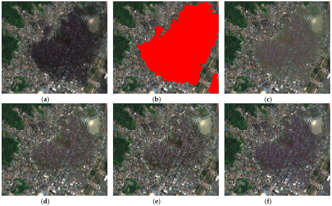
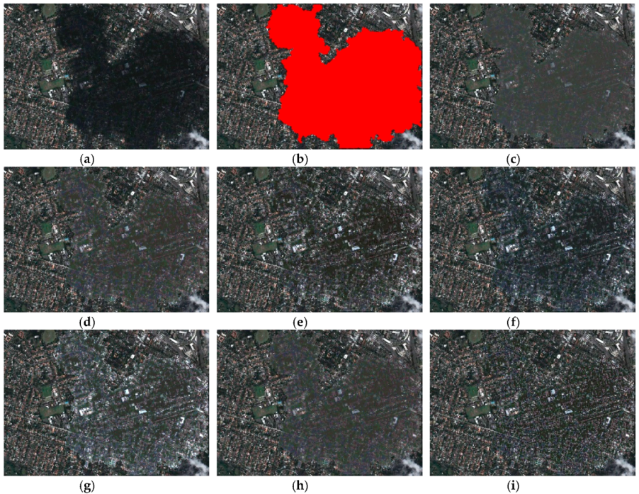
The cloud shadow compensation comparison results effectively show the difference in a single shadow area. Figure 4, Figure 5 and Figure 6 show that our method obtained better results in brightness, contrast, and original colors than the other methods. OWC’s results indicate that the brightness was rising while the contrast was almost unchanging. LCC, GMC, HMT, CRM, and OOPR improved both the brightness and contrast to some extent and the original color of the objects in the shadow areas was recovered (e.g., the trees in Figure 4 are depicted in their true green color). HMT produced the best and most stable capability for improving the contrast while the other methods’ contrast indicated another problem of uneven compensation in a single shadow area. The part of the cloud shadow area that was obscured by the thicker cloud is still slightly darker than the thinner part after compensation in almost all the reference methods. In comparison, this uneven compensation problem was solved by the multilevel combination strategy. For the bare land in Figure 5, there is a small non-shadow region that is recognized as shadows. This part was easily overcompensated by other methods, but our method addressed this phenomenon because its local window information was useful in adaptively enhancing each partially shaded information to the same level as the non-shadow area. Thus, our model recovered the information as accurately as possible and showed almost no difference in comparison to the non-shadow areas.
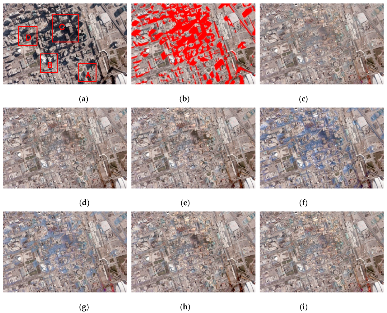
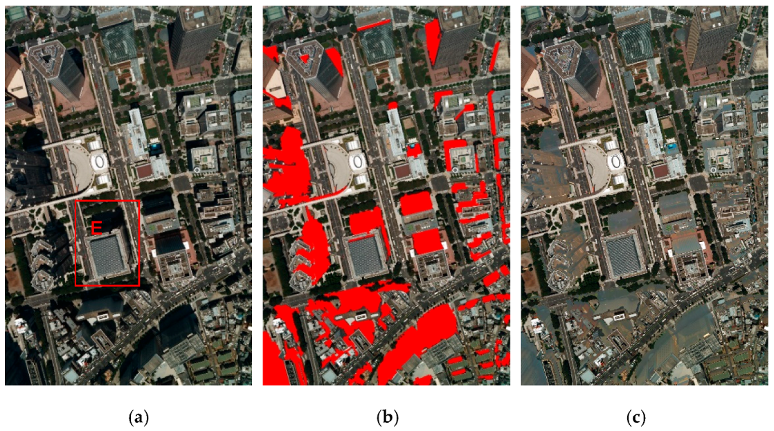
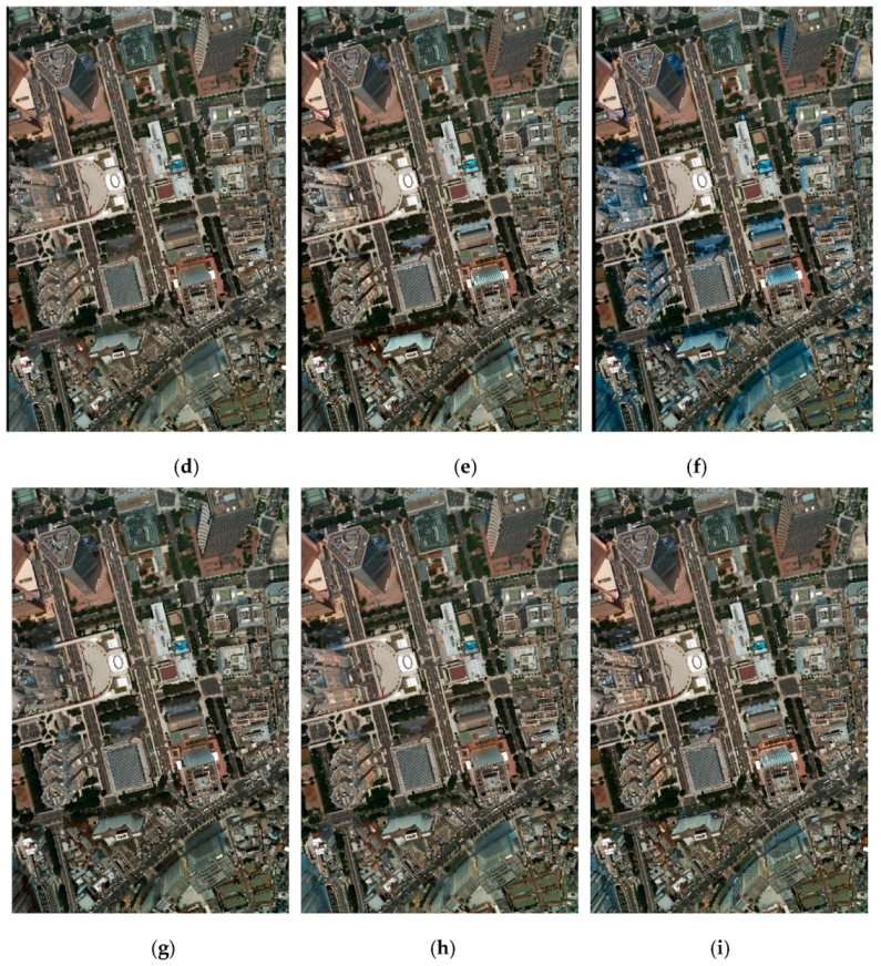
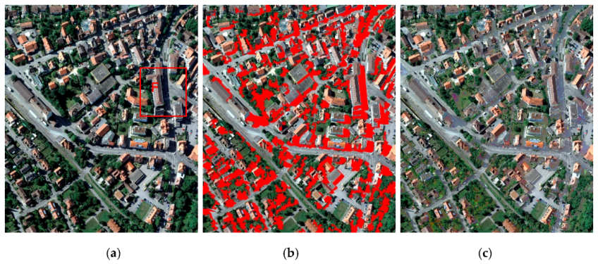
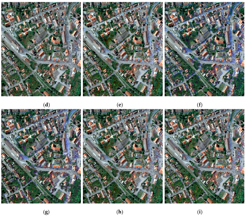
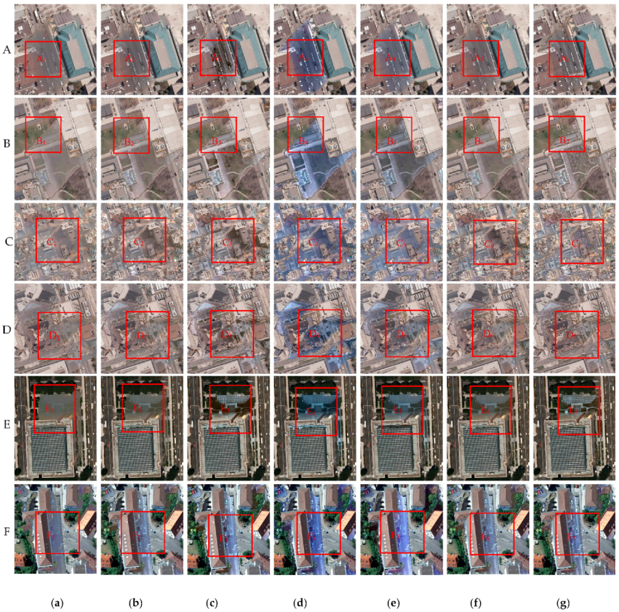
Regarding ground object shadow compensation, our method produced better results, which indicated its ability to compensate for each shadow region. Different shadow regions were improved and were identical to their adjacent non-shadow areas, which was beneficial for avoiding over-compensation or insufficient compensation. Even though the object information shaded by the buildings was too dark to see, our method recovered the information. To depict the compensation results of our method in detail, six portions of Images 4–6 in Figure 7, Figure 8 and Figure 9 were selected, which are named A-F in Figure 10. From the figures and Table 1, it can be seen that our method produced better visual and quantitative compensation results than the other methods.
When compared to the non-adaptive methods (OWC, GMC, HMT, and LCC), our approach was able to compensate for shadows more adaptively. Although OWC significantly enhanced the brightness, the shadow areas were still unclear for less heightened contrast. GMC also improved the brightness and contrast efficiently; and while its contrast enhancement was better than OWC, it was not as good as the other methods, as shown in boxes B2, E2, and F2. Because parameter γ could not be adaptive to every image and shadow area, it was hard to decide which value was best for them. Therefore, GMC’s compensation capability was not stable and self-adaptive. The effect of GMC was different among the images; and therefore, sometimes it was good, as seen in Images 2 and 5, but mostly it was not good enough. HMT produced stable compensation results and was especially good at contrast enhancement; however, sometimes it was over-enhanced and lost the original information. As can be seen in box A3, the shadow area was over-compensated in contrast. Comparatively, LCC, as one of the most typical compensation methods, undeniably recovered the primary information in the shadow area; and while it enhanced brightness and contrast efficiently, it was unable to achieve the same levels as in the non-shadow areas. LCC also produced color deviation and uneven improvements in different shadow areas; and its results show a blue color instead of the original color. This color difference was mainly caused by its over-enhanced illumination, resulting in a higher blue component than the non-shadow area. However, the color bios in cloud shadow were less serious than the ground object shadows since the difference between the compensated shadow area and the non-shadow area was low. In comparison, the results for our method represented the original roof color better due to our color correction strategy. Additionally, the problem of uneven compensation was present in most of the compared methods (e.g., the boxes in Images C and D). Box C4 shows that LCC experienced inefficient and uneven compensation.
Recent methods, such as OOPR and CRM, were designed to obtain self-adaptive parameters adjusted according to each shadow as well. Although they adopted their respective adaptive parameter strategies, they did not achieve stable results in the various images. OOPR utilizes a polynomial fitting compensation principle, which cannot solve the best function for each shadow region from the IPOOL strategy. As a result, OOPR improved the brightness similarity to the non-shadow area, but its contrast enhancement was inadequate due to its limited polynomial function. As shown in Image 3, the brightness was satisfied while the contrast did not meet the non-shadow level. In addition, although CRM also utilizes LCC as the compensation model, it gained the non-shadow information from the adjacent non-shadow segment areas of each shadow area. CRM produced overcompensation as shown in Image 4, Image C, and Image F. For example, the shadow in box F5 is obviously over-compensated; and the contrast enhancement in Image F is worse than in Images C and D. When the segmentation areas were not suitable, the shadow area was over-compensated or insufficiently compensated, as shown in Image F. It is difficult to both improve the brightness and contrast at the same time in a way that is similar to non-shadow areas, which was a common problem for CRM and OOPR.
In contrast, these problems were solved by our method, since it was able to adaptively recover the shaded information as clearly and initially as it would appear in sunlight. Since our approach uses different parameters for different shadow areas, the shadow information is strengthened more reasonably according to every shadow situation. The most significant benefit of this strategy is that it prohibits over-compensation or inefficient compensation. Moreover, using the local window compensation, the details in each shadow area are more evenly promoted.

4.4. Quantitative Comparison

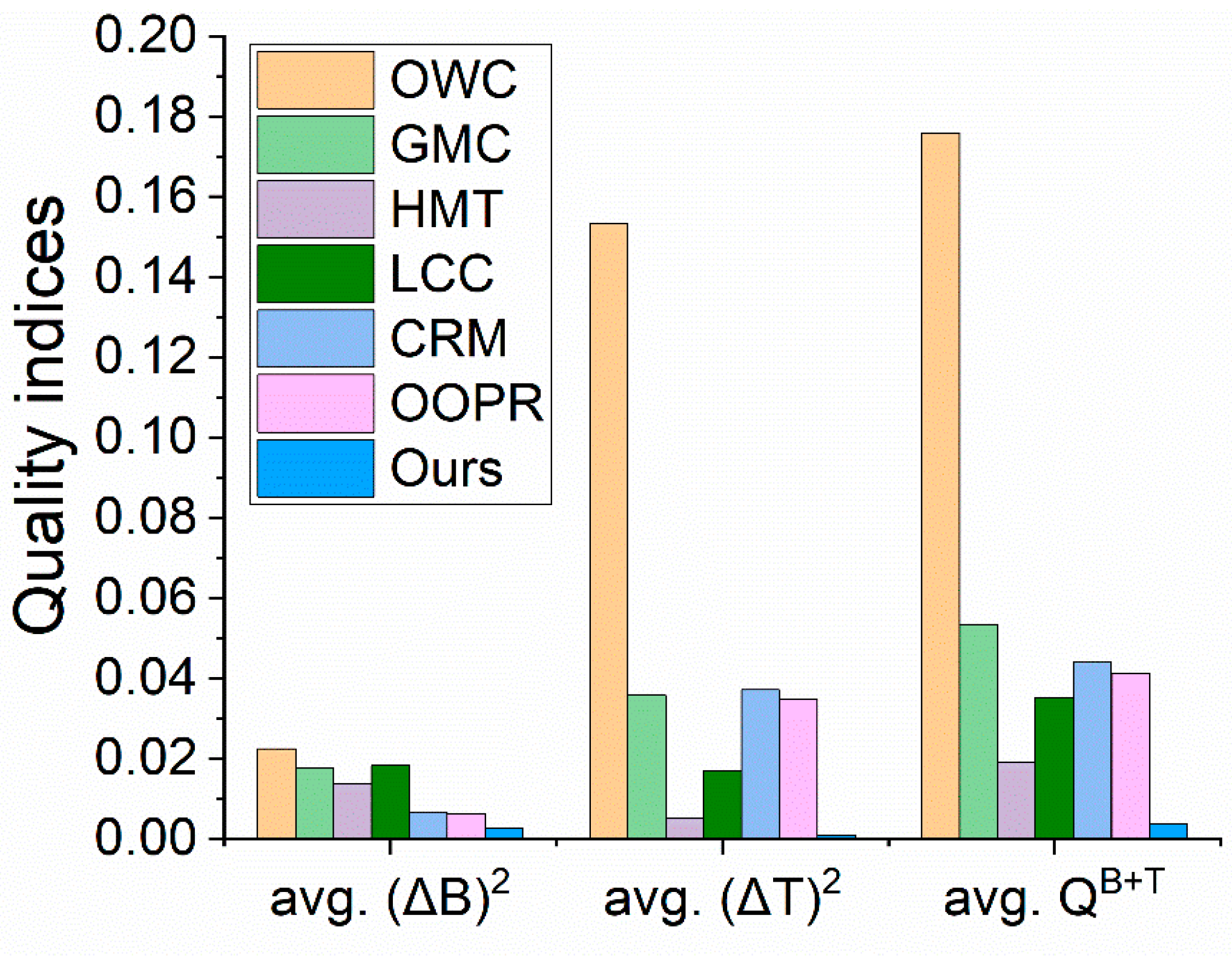
In the quantitative comparison, our method achieved the best compensation quality image measured by QB+T. The reinforcement of T was closer to the non-shadow area while the average brightness was slightly lower than that of the non-shadow area; and the total compensation quality was much better than the other methods as well. Figure 11 shows the 25 images that were tested and compares the average of ( Δ B ) 2 , ( Δ T ) 2 , and QB+T they achieved. The results were analyzed by combining visual and quantitative outcomes. The average QB+T of our method in Figure 11 and Table 1 were 0.0038 and 0.0021, respectively. Both values indicate the same conclusion, namely, that our method produced the best compensation results, followed by the HMT method with 0.0099, and then the LCC with 0.0268. The OWC method attained the worst results due to its low capability in enhancing contrast. The other methods were not very stable. Since the QB+T cannot reflect the color deviation and the even contrast detail in a single shadow area, the methods’ results differed visually, as shown in Figure 4, Figure 5, Figure 6, Figure 7, Figure 8, Figure 9 and Figure 10.
In summary, the comparative results indicate that our method enlarged the shaded information from low quality to a quality that was close to the non-shaded area in brightness and contrast in a more balanced way. Additionally, our method recovered the color information and self-adaptively constructed the compensation model, resulting in more even enhancement and better recovery of the original information of the shadow objects.

4.5. Time Computation

The proposed method was implemented in a VS2019 environment using a hybrid program code based on C++ and OpenCV. All the experiments were conducted on a laptop with an Intel Core i7 CPU, 2.60 GHz, and 32 GB RAM. The computation times for all the compared methods are shown in Table 2. The time of GMC and HMT was similar, and they were the shortest because they adopt the same parameter value to the whole shadow areas in an image. OWC and LCC use the mean and variance of each shadow area, which resulted in longer computation times. CRM requires segmentation results in order to obtain the non-shadow region information; therefore, it required the longest time to accomplish shadow compensation. Both our method and OOPR solved the parameter values for each shadow; but because OOPR adopts an IPOOL strategy, it is more complicated than our approach and therefore required a little more time. Although our method’s computation time was moderate but not the fastest, it accomplished a better compensation result for each shadow area.

5. Discussions

To evaluate the capability of the proposed method more specifically, we analyzed the impact of the introduced coefficient α and β on the compensation quality indexes and the effectiveness of the automatic calculation strategy.

5.1. The Positive Impact of α and β on the Proposed Model

Taking I as an example, the compensation experiment continued on the shadow image TIGS in Figure 2a and TICS in Figure 2c to verify the influence of α and β. A comparison of the compensation results by assigning different values to α and β was implemented, as visually shown in Table 3 and Table 4. The figures in the table show how the brightness and contrast changes with the change of the parameter. When fixing β and changing α in compensation model of Equation (5), B and T are both improved with the increase of α; when fixing α and changing β, T decreases, and B remains unchanged with the rise of β.
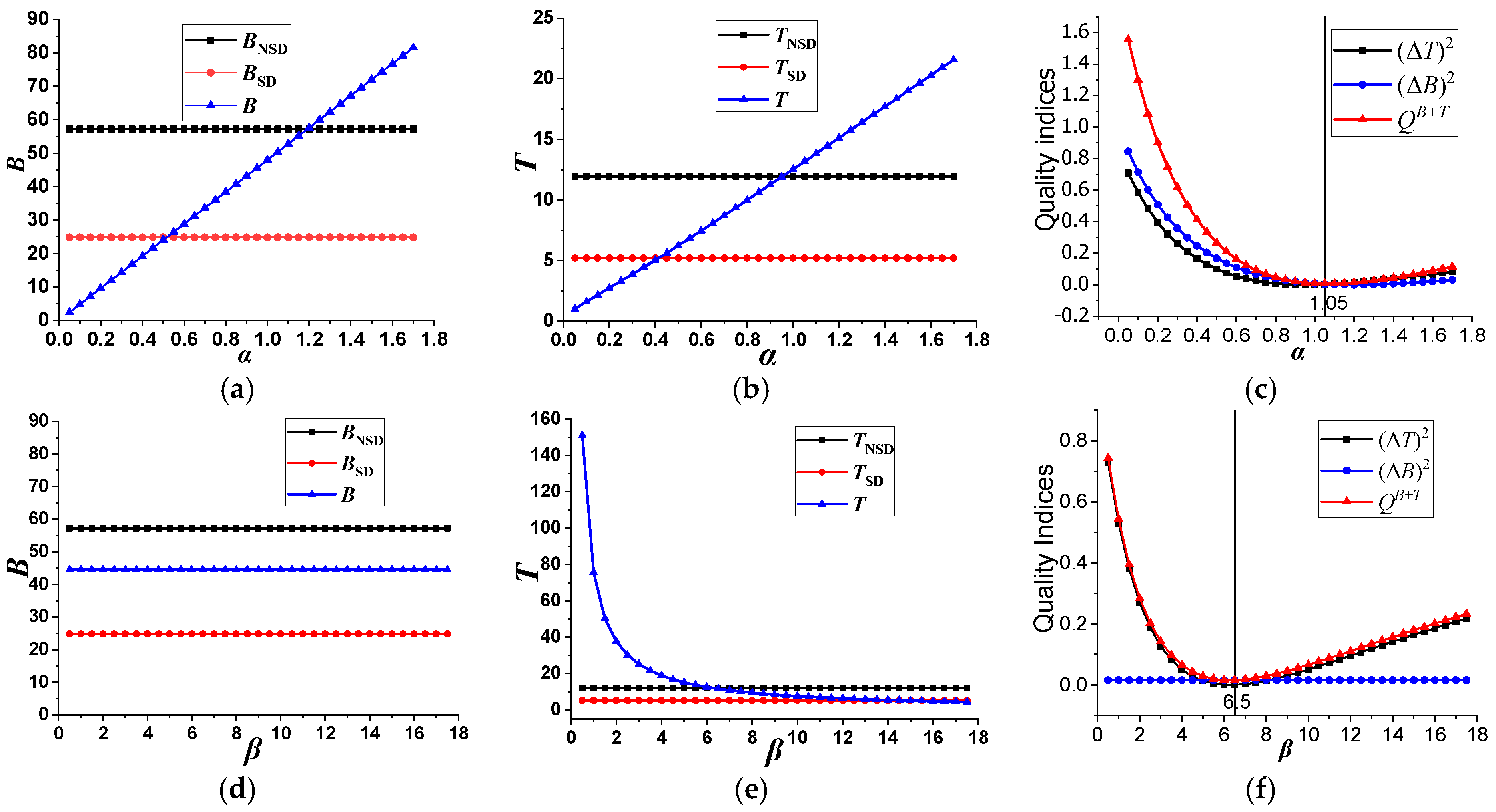
Figure 12 describes the influence of α and β on the compensation results. Figure 12a,b show that α affects both B and T linearly and positively. However, for the values for α that were too high, the brightness and contrast compensation was excessive, while the values that were too low for α made the brightness and contrast compensation insufficient. As shown Figure 12c, with the increasing value of α, (ΔB)2 and (ΔT)2 decreased until they reached the lowest points; and the increasing α led to an increase in (ΔB)2 and (ΔT)2. Hence, selecting an optimal value for α was important to achieve a target compensation value. The best solution was to acquire the α value, where QB+T achieved the minimum. β had little influence on B, and it only affected the T of the shadow area nonlinearly and negatively, as shown in Figure 12d,e, respectively. Meanwhile, the impacts of β on (ΔB)2 and (ΔT)2 were similar to the impacts on B and T. With the increase of β, (ΔT)2 decreased greatly and flattened. Therefore, β was effective for strengthening T (the contrast) more efficiently. If a suitable value of β was selected based on the lowest QB+T, the information about the shadow area was restored. Thus, both α and β had a positive impact on compensation quality. The lowest QB+T pinned down the best value of α and β, which helped to achieve brightness and contrast similar to the non-shadow target.

5.2. The Effectiveness of the Automatic Strategy for α and β Calculation

The automatic strategy for α and β calculation is important for accomplishing automatic compensation without manual direction. It also helps customize suitable compensation models for each shadow area but not for the whole image. In order to verify the effectiveness of the automatic parameter strategy, four different shadow areas were tested to compare the optimal values acquired by the minimum QB+T with the automatic values of α and β. The relationship between QB+T and α as well as QB+T and β, as shown in Figure 13, were used to estimate the ideal values of α and β at the minimum QB+T. Furthermore, the automatic values of α and β calculated by the strategy are shown in Table 5. The comparison results show that the automatic calculation value was close to the estimated ideal value for both α and β, which indicates that the parameter calculation strategy effectively calculated the suitable values for the compensation parameters. As a result, those values were effective in customizing a suitable model for each shadow.

5.3. Validation for Color Correction

Since our method can be used to heighten any component to recover the shadow information, choosing efficient components to raise the shadow information closer to its original content is significant. In general, H, S, and I were all used together to compensate in several studies, but this approach is not effective for maintaining the original color of the shadow objects. Because it almost raises all of the components to similar values, the results show a gray color that does not reflect the original colors, as shown in Figure 14a,d. In fact, during the experiments and in our previous research [31], component I was rather efficient for cloud shadows compensation to recover the original information, leading to some color loss in ground object shadows compensation. As shown in Figure 14b,e, the results were greater with the proposed model for compensating component I; and within the building shadows, there is a color deviation from the original color that does not occur in the cloud shadow compensation results. As shown in Figure 14c,f, the results optimized by the color correction strategy show the original colors were well maintained.

6. Conclusions

This paper introduced and demonstrated the implementation of a new shadow compensation model that combines the Wallis filtering principle and LCC model by adding intensity coefficient α and stretching coefficient β to adjust brightness and contrast effectively. When combined with a parameter automatic extraction scheme based on feature point pairs, our method was found to target loss information more accurately; and the compensation parameters in our model were able to be obtained automatically. By combining the local window and a regional compensation model, using a multilevel combination strategy, the shaded information was evenly enhanced as well. As shown in this paper, when compared to other state-of-the-art methods, our contrast and brightness enhancements produced better and more consistent results for the non-shadow areas. They were able to restore the real information of the features shaded by shadows. Our model’s shadow-free, higher-quality images demonstrate its image reconstruction capabilities and its potential for use in complete land-cover or land-use map applications.

Author Contributions

Y.Y., X.G. and S.R. conceived and conducted the experiments, and performed the data analysis, M.W. and X.L. revised the manuscript; Y.Y. and X.G. wrote the article. All authors have read and agreed to the published version of the manuscript.

Funding

This work is supported in part by Open Fund of State Laboratory of Information Engineering in Surveying, Mapping and Remote Sensing, Wuhan University, China, under Grant 18R04, and in part by Scientific research program of Hubei provincial department of education, China, under Grant Q20181317.

Acknowledgments

Part of the work was completed when Gao was visiting Purdue University and had insightful discussions with Jie Shan. All authors would like to thank Shan and the anonymous reviewers whose insightful suggestions have improved the paper significantly.

Conflicts of Interest

The authors declare no conflict of interest.

References

  1. Mostafa, Y. A review on various shadow detection and compensation techniques in remote sensing images. Can. J. Remote Sens. 2017, 43, 545–562. [Google Scholar] [CrossRef]
  2. Chai, D.; Newsam, S.; Zhang, H.K.; Qiu, Y.; Huang, J. Cloud and cloud shadow detection in Landsat imagery based on deep convolutional neural networks. Remote Sens. Environ. 2019, 225, 307–316. [Google Scholar] [CrossRef]
  3. Li, Z.; Shen, H.; Li, H.; Xia, G.; Gamba, P.; Zhang, L. Multi-feature combined cloud and cloud shadow detection in GaoFen-1 wide field of view imagery. Remote Sens. Environ. 2017, 191, 342–358. [Google Scholar] [CrossRef] [Green Version]
  4. Lv, Z.Y.; Liu, T.F.; Zhang, P.; Benediktsson, J.A.; Lei, T.; Zhang, X. Novel adaptive histogram trend similarity approach for land cover change detection by using bitemporal very-high-resolution remote sensing images. IEEE Trans. Geosci. Remote Sens. 2019, 57, 9554–9574. [Google Scholar] [CrossRef]
  5. Gao, X.; ang, M.; Yang, Y.; Li, G. Building Extraction From RGB VHR Images Using Shifted Shadow Algorithm. IEEE Access 2018, 6, 22034–22045. [Google Scholar] [CrossRef]
  6. Sarabandi, P.; Yamazaki, F.; Matsuoka, M.; Kiremidjian, A. Shadow detection and radiometric restoration in satellite high resolution images. In Proceedings of the 2004 IEEE International Geoscience and Remote Sensing Symposium (IGARSS’04), Anchorage, AK, USA, 20–24 September 2004; pp. 3744–3747. [Google Scholar]
  7. Wang, S.; Wang, Y. Shadow detection and compensation in high resolution satellite image based on retinex. In Proceedings of the 2009 Fifth International Conference on Image and Graphics, Xi’an, China, 20–23 September 2009; pp. 209–212. [Google Scholar]
  8. Jobson, D.J.; Rahman, Z.-U.; Woodell, G.A. Properties and performance of a center/surround retinex. IEEE Trans. Image Process. 1997, 6, 451–462. [Google Scholar] [CrossRef]
  9. Ma, H.; Qin, Q.; Shen, X. Shadow segmentation and compensation in high resolution satellite images. In Proceedings of the IGARSS 2008 IEEE International Geoscience and Remote Sensing Symposium, Boston, MA, USA, 8–11 July 2008; pp. II-1036–II-1039. [Google Scholar]
  10. Liu, J.; Fang, T.; Li, D. Shadow detection in remotely sensed images based on self-adaptive feature selection. IEEE Trans. Geosci. Remote Sens. 2011, 49, 5092–5103. [Google Scholar]
  11. Tiwari, K.C.S.; Kurmi, Y. Shadow detection and compensation in aerial images using MATLAB. Int. J. Comput. Appl. 2015, 119, 5–9. [Google Scholar] [CrossRef]
  12. Wang, W. Study of Shadow Processing’s Method High-Spatial Resolution RS Image. Master’s Thesis, Xi’an University of Science and Technology, Xi’an, China, 2008. [Google Scholar]
  13. Liu, W.; Yamazaki, F. Object-based shadow extraction and correction of high-resolution optical satellite images. IEEE J. Sel. Top. Appl. Earth Obs. Remote Sens. 2012, 5, 1296–1302. [Google Scholar] [CrossRef]
  14. Luo, S.; Li, H.; Shen, H. Shadow removal based on clustering correction of illumination field for urban aerial remote sensing images. In Proceedings of the 2017 IEEE International Conference on Image Processing (ICIP), Beijing, China, 17–20 September 2017; pp. 485–489. [Google Scholar]
  15. Tsai, V.J. A comparative study on shadow compensation of color aerial images in invariant color models. IEEE Trans. Geosci. Remote Sens. 2006, 44, 1661–1671. [Google Scholar] [CrossRef]
  16. Jian, Y.; He, Y.; Caspersen, J. Fully constrained linear spectral unmixing based global shadow compensation for high resolution satellite imagery of urban areas. Int. J. Appl. Earth Obs. Geoinf. 2015, 38, 88–98. [Google Scholar]
  17. Nair, V.; Ram, P.G.K.; Sundararaman, S. Shadow detection and removal from images using machine learning and morphological operations. J. Eng. 2019, 2019, 11–18. [Google Scholar] [CrossRef]
  18. Vicente, T.F.Y.; Hoai, M.; Samaras, D. Leave-one-out kernel optimization for shadow detection and removal. IEEE Trans. Pattern Anal. Mach. Intell. 2018, 40, 682–695. [Google Scholar] [CrossRef] [PubMed]
  19. Zigh, E.; Belbachir, M.F.; Kadiri, M.; Djebbouri, M.; Kouninef, B. New shadow detection and removal approach to improve neural stereo correspondence of dense urban VHR remote sensing images. Eur. J. Remote Sens. 2015, 48, 447–463. [Google Scholar] [CrossRef]
  20. Ibrahim, I.; Yuen, P.; Hong, K.; Chen, T.; Soori, U.; Jackman, J.; Richardson, M. Illumination invariance and shadow compensation via spectro-polarimetry technique. Opt. Eng. 2012, 51. [Google Scholar] [CrossRef] [Green Version]
  21. Roper, T.; Andrews, M. Shadow modelling and correction techniques in hyperspectral imaging. Electron. Lett. 2013, 49, 458–459. [Google Scholar] [CrossRef]
  22. Wan, C.Y.; King, B.A.; Li, Z. An Assessment of Shadow Enhanced Urban Remote Sensing Imagery of a Complex City-Hong Kong. In Proceedings of the International Archives of the Photogrammetry, Remote Sensing and Spatial Information Sciences XXII ISPRS Congress, Melbourne, Australia, 25 August 2012; pp. 177–182. [Google Scholar]
  23. Mo, N.; Zhu, R.; Yan, L.; Zhao, Z. Deshadowing of urban airborne imagery based on object-oriented automatic shadow detection and regional matching compensation. IEEE J. Sel. Top. Appl. Earth Obs. Remote Sens. 2018, 11, 585–605. [Google Scholar] [CrossRef]
  24. Luo, S.; Shen, H.; Li, H.; Chen, Y. Shadow removal based on separated illumination correction for urban aerial remote sensing images. Signal Process. 2019, 165, 197–208. [Google Scholar] [CrossRef]
  25. Wang, C.; Xu, H.; Zhou, Z.; Deng, L.; Yang, M. Shadow detection and removal for illumination consistency on the road. IEEE Trans. Intell. Veh. 2020. [Google Scholar] [CrossRef]
  26. Chen, Y.; Wen, D.; Jing, L.; Shi, P. Shadow information recovery in urban areas from very high resolution satellite imagery. Int. J. Remote Sens. 2007, 28, 3249–3254. [Google Scholar] [CrossRef]
  27. Mostafa, Y.; Abdelwahab, M.A. Corresponding regions for shadow restoration in satellite high-resolution images. Int. J. Remote Sens. 2018, 39, 7014–7028. [Google Scholar] [CrossRef]
  28. Liang, D.; Kong, J.; Hu, G.; Huang, L. The removal of thick cloud and cloud shadow of remote sensing image based on support vector machine. Acta Geod. Cartogr. Sin. 2012, 41, 225–231+238. [Google Scholar]
  29. Zhang, H.Y.; Sun, K.M.; Li, W.Z. Object-oriented shadow detection and removal from urban high-resolution remote sensing images. IEEE Trans. Geosci. Remote Sens. 2014, 52, 6972–6982. [Google Scholar] [CrossRef]
  30. Friman, O.; Tolt, G.; Ahlberg, J. Illumination and shadow compensation of hyperspectral images using a digital surface model and non-linear least squares estimation. In Proceedings of the Image and Signal Processing for Remote Sensing XVII 2011, Prague, Czech Republic, 26 October 2011; pp. 81800Q–81808Q. [Google Scholar]
  31. Gao, X.; Wan, Y.; Yang, Y.; He, P. Automatic shadow detection and automatic compensation in high resolution remote sensing images. Acta Autom. Sin. 2014, 40, 1709–1720. [Google Scholar]
  32. Huang, X.; Zhang, L. Morphological building/shadow index for building extraction from high-resolution imagery over urban areas. IEEE J. Sel. Top. Appl. Earth Obs. Remote Sens. 2012, 5, 161–172. [Google Scholar] [CrossRef]
  33. Jiménez, L.I.; Plaza, J.; Plaza, A. Efficient implementation of morphological index for building/shadow extraction from remotely sensed images. J. Supercomput. 2017, 73, 482–494. [Google Scholar] [CrossRef]
  34. Otsu, N. Threshold selection method from gray-level histograms. IEEE Trans. Syst. Man Cybern. 1979, 9, 62–66. [Google Scholar] [CrossRef] [Green Version]
  35. Fan, C.; Chen, X.; Zhong, L.; Zhou, M.; Shi, Y.; Duan, Y. Improved wallis dodging algorithm for large-scale super-resolution reconstruction remote sensing images. Sensors 2017, 17, 623. [Google Scholar] [CrossRef] [Green Version]
  36. Tian, J.; Li, X.; Duan, F.; Wang, J.; Ou, Y. An efficient seam elimination method for UAV images based on wallis dodging and gaussian distance weight enhancement. Sensors 2016, 16, 662. [Google Scholar] [CrossRef]
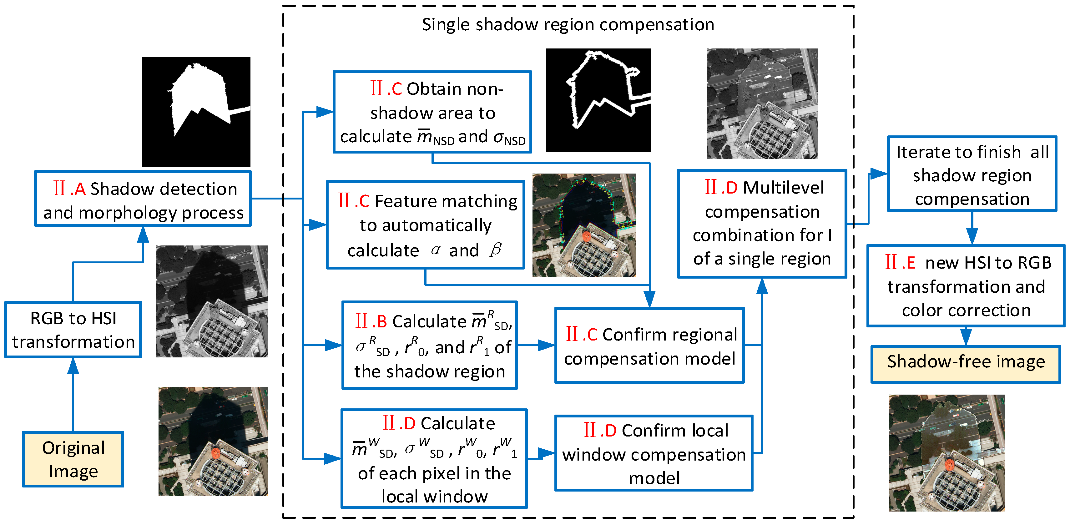
Figure 1. Flow chart of automatic shadow compensation.
Applsci 10 05799 g001
Figure 2. Shadow compensation results by the original Wallis filter principle. (a) Test Image of Ground object Shadows, named TIGS; (b) Original Wallis compensation results of TIGS; (c) Test Image of a Cloud Shadow, named TICS; (d) Original Wallis compensation results of TICS.
Applsci 10 05799 g002
Figure 3. Feature points acquisition and relative regions schematic diagram for automatic compensation. (a) Compensation related areas. (b) Similar feature point pairs.
Applsci 10 05799 g003
Figure 4. Cloud shadow compensation results in satellite Image 1. (a) Original image; (b) Shadow detection result (red); (c) The OWC result; (d) The GMC result; (e) The HMT result;(f) The LCC result; (g) The CRM result; (h) The OOPR result; (i) Our method’s result.
Applsci 10 05799 g004
Figure 5. Cloud shadow compensation results in satellite Image 2. (a) Original image; (b) Shadow detection result (red); (c) The OWC result; (d) The GMC result; (e) The HMT result;(f) The LCC result; (g) The CRM result; (h) The OOPR result; (i) Our method’s result.
Applsci 10 05799 g005aApplsci 10 05799 g005b
Figure 6. Cloud shadow compensation results in satellite Image 3. (a) Original image; (b) Shadow detection result (red); (c) The OWC result; (d) The GMC result; (e) The HMT result; (f) The LCC result; (g) The CRM result; (h) The OOPR result; (i) Our method’s result.
Applsci 10 05799 g006
Figure 7. Shadow compensation results in aerial Image 4. (a) Original image; (b) Shadow detection result (red); (c) The OWC result; (d) The GMC result; (e) The HMT result;(f) The LCC result; (g) The CRM result; (h) The OOPR result; (i) Our method’s result.
Applsci 10 05799 g007
Figure 8. Shadow compensation results in aerial Image 5. (a) Original image; (b) Shadow detection result (red); (c) The OWC result; (d) The GMC result; (e) The HMT result;(f) The LCC result; (g) The CRM result; (h) The OOPR result; (i) Our method’s result.
Applsci 10 05799 g008aApplsci 10 05799 g008b
Figure 9. Shadow compensation results in aerial Image 6. (a) Original image; (b) Shadow detection result (red); (c) The OWC result; (d) The GMC result; (e) The HMT result;(f) The LCC result; (g) The CRM result; (h) The OOPR result; (i) Our method’s result.
Applsci 10 05799 g009aApplsci 10 05799 g009b
Figure 10. Shadow compensation results in detail. (a) OWC; (b) GMC; (c) HMT; (d) LCC; (e) CRM; (f) OOPR; (g) Our Method.
Applsci 10 05799 g010
Figure 11. Comparison for the average of quality indices of 25 test images.
Applsci 10 05799 g011
Figure 12. The influence of intensity coefficient α and stretching coefficient β on the compensation quality. BSD and TSD, BNSD, and TNSD are the brightness average and the average gradient of the shadow area and the non-shadow area. B and T are the compensated values in the shadow area. (ΔB)2 and (ΔT)2 are the square of the normalized difference between the compensated value and the non-shadow area in B and T, respectively. QB+T is the total compensation quality. (a) Relationship between α and average brightness B; (b) Relationship between α and average gradient T; (c) The effect of α on (ΔB)2, (ΔT)2, and QB+T; (d) Relationship between β and B; (e) Relationship between β and T; (f) The effect of β on (ΔB)2, (ΔT)2, and QB+T.
Applsci 10 05799 g012
Figure 13. Relationships between compensation parameters and quality in different regions. (a) Relationship between α and QB+T; (b) Relationship between β and QB+T.
Applsci 10 05799 g013
Figure 14. Comparison of the proposed compensation results using different color correction strategies in Figure 2a,c. (a) Building shadow compensation result for components H, I, and S of Figure 2a; (b) Building shadow compensation result for component I; (c) Building shadow compensation result after color correction; (d) Cloud shadow compensation result for component H, I, and S of Figure 2c; (e) Cloud shadow compensation for component I; (f) Cloud shadow compensation result after color correction.
Applsci 10 05799 g014
Table 1. The evaluation comparison of compensation results in Figure 4, Figure 5, Figure 6, Figure 7, Figure 8, Figure 9 and Figure 10.
Image NameQuality
Index
SDNSDOWCGMCHMTLCCCRMOOPROurs
1B36.275463.188958.792062.029963.271362.777173.441777.732763.7444
T5.183914.44095.74899.367311.35959.29008.284413.229514.2704
QB+T0.18660.04550.01430.04710.07900.01260.0001
2B57.935985.108583.248182.460091.872786.986097.142794.955987.5762
T7.890716.28619.611013.098913.827411.012210.276911.721715.0647
QB+T0.06660.01200.00810.03740.05550.02950.0017
3B37.000874.314261.547873.181772.765966.792486.172376.853371.7967
T4.900323.77734.898011.349719.781317.546221.992810.354221.7824
QB+T0.44230.12520.00850.02560.00700.15490.0022
4B56.9910150.1633124.6353116.4057133.0205124.2297155.2552160.0377149.8764
T10.868020.619113.311817.808321.349913.311835.546621.385721.0447
QB+T0.05500.02140.00400.05530.07090.00130.0001
5B24.659191.968065.774471.305673.049268.074581.709989.309582.5732
T5.574222.167210.418416.548622.139819.086215.651117.778123.2122
QB+T0.15760.03710.01310.02790.03320.01230.0034
6B23.4614107.772272.742263.796780.888874.7187129.513366.239896.0105
T10.562921.530711.193620.714525.604321.138744.530320.561723.9488
QB+T0.13740.06610.02780.03290.12960.05750.0062
AB52.7057148.7910107.6152109.4551121.2661113.6874105.1475127.9258131.1461
T6.716916.98519.511613.437818.851715.567312.691111.092617.1362
QB+T0.10530.03680.01310.01980.05050.04970.0040
BB52.0459149.1248113.8646117.4061136.1765127.4515107.5620140.2063139.5191
T4.080313.43225.38788.470813.966712.048310.56628.764213.8181
QB+T0.20070.06550.00240.00910.04050.04520.0013
CB50.3020136.3924116.0753105.9343121.3617112.6049142.1750135.7543135.5174
T7.038821.52838.536211.980719.467115.519825.851913.658521.2531
QB+T0.19320.09700.00590.03540.00880.05000.0001
DB54.6436142.2926105.7497120.4303121.9426114.5220115.9803142.4835129.9071
T4.928515.20545.995910.250715.780214.172610.909410.515515.3493
QB+T0.21040.04480.00630.01290.03740.03320.0021
EB22.151390.683872.601271.689581.109776.122273.871791.919988.5145
T2.818220.49058.783214.822420.303618.653916.332411.466120.5716
QB+T0.17220.03940.00310.00980.02320.07980.0002
FB22.1948116.934284.340271.496195.599387.6406112.308886.5574102.5739
T6.421318.44007.306514.679421.053917.735230.742616.633517.2710
QB+T0.21320.07100.01450.02090.06300.02490.0054
Average QB+T0.19150.05810.00990.02680.05570.05000.0021
Table 2. Shadow compensation time comparison of different images in Figure 4, Figure 5, Figure 6, Figure 7, Figure 8, Figure 9 and Figure 10.
Image NameShadow Rate
(%)
Length × Width
(pixel)
OWC
(s)
GMC
(s)
HMT
(s)
LCC
(s)
CRM
(s)
OOPR
(s)
Ours
(s)
150.563823×5760.0750.0330.0340.1794.6271.1020.893
238.979686×6010.0760.0380.0330.0821.6500.8890.677
345.893894×6340.1430.0650.0640.1592.3361.6041.338
426.7831437×9370.2970.1720.1860.37533.4695.0344.688
522.352937×14370.1860.1050.1080.23420.2761.9031.641
627.0771004×11880.2630.1290.1290.26932.8861.5251.264
Table 3. Comparison of results compensation for TIGS and TICS by fixing β = 10 and applying different α in Equation (5).
α = 0.5α = 0.75α = 1α = 1.25
β = 10 Applsci 10 05799 i001 Applsci 10 05799 i002 Applsci 10 05799 i003 Applsci 10 05799 i004
Applsci 10 05799 i005 Applsci 10 05799 i006 Applsci 10 05799 i007 Applsci 10 05799 i008
Table 4. Comparison of results compensation for TIGS and TICS by fixing α = 0.95 and applying different β in Equation (5).
β = 5β = 10β = 15β = 20
α = 0.95 Applsci 10 05799 i009 Applsci 10 05799 i010 Applsci 10 05799 i011 Applsci 10 05799 i012
Applsci 10 05799 i013 Applsci 10 05799 i014 Applsci 10 05799 i015 Applsci 10 05799 i016
Table 5. Comparison of α and β values calculated automatically with its ideal value of different regions.
Area Nameα Automatic Valueβ Automatic Valueα Ideal Valueβ Ideal Value
11.2951.0361.351
21.2640.9261.31
31.0919.8311.110
41.08636.3211.056.5