3D Reconstruction of a Single Bubble in Transparent Media Using Three Orthographic Digital Images

Abstract

This work proposed a method to reconstruct the 3D bubble shape in a transparent medium utilizing the three orthographic digital images. The bubble was divided into several ellipse slices. The azimuth angle and projection parameters were extracted from the top view image, while the formulas for dimensionless semi-axes were derived according to the geometric projection relationship. The elliptical axes of each layer were calculated by substituting the projection width into the formulas. All layers of slices were stacked to form the 3D bubble shape. Reconstruction accuracy was evaluated with spheres, ellipsoids, and inverted teardrops. The results show that the position contributes greatly to the reconstruction accuracy of the bubbles with serious horizontal deformation. The method in Bian et al. (2013) is sensitive to both horizontal and vertical deformations. The vertical deformation has little influence on the method in Fujiwara et al. (2004), whereas the horizontal deformation greatly impacts its accuracy. The method in this paper is negligibly affected by vertical deformation, but it does better in reconstructing single bubbles with large horizontal deformation. The azimuth angle affects the accuracy of the methods in Bian et al. (2013) and Fujiwara et al. (2004) more than the method in this paper.

1. Introduction

Studying the hydrodynamics of a single bubble growth and detachment in motionless fluids always attracts researchers [1,2]. The literature of a single bubble generated in Newtonian fluids has been studied for decades and this well-known classic work was published, [3]. Despite the importance of this problem, many applications are dealing with bubbles in non-Newtonian fluids, and bubbles in such fluids have not been thoroughly studied. Recently, some studies focused on the dependence of the single bubble shape on their dynamics such as velocity discontinuity, as well as on the contact angle, viscosity, and surface tension [4,5]. To this end, the 3D bubble shape reconstruction is vital for the further analysis of hydrodynamic interactions among a single bubble and surrounding liquid.

There exists a significant body of scientific research discussing the calculation of bubble size and its formation. Early researchers used the balance formula of buoyancy and surface tension to calculate the volume of a single bubble [6]. Then, the Rayleigh-Plesset equation [7,8] and Young-Laplace equation [9,10] were utilized to predict the formation of bubbles. Many numerical simulation techniques, including the boundary integral method [11], the finite element analysis method [12] have also been applied to forecasting bubble formation. In general, the results of theoretical calculations and numerical simulations need to be verified by accurate experimental data. Therefore, a method which could precisely extract 3D bubble formation from orthographic images can be employed to validate the rationality of various theoretical calculation methods and numerical simulation techniques.

With the progressive development of technology, advanced measuring equipment has been employed to study the bubble visualization. Although the distribution of bubbles can be obtained by destructive measurements such as probes [13], invaded probes interfere in the motion of bubbly flows to some extent. Therefore, noninvasive measurement techniques such as electrical tomography [14], interference technology [15], laser tomography [16], and optical imaging [17] have widely been utilized since they have no effect on fluid structure. Among these techniques, the optical imaging technology can completely and conveniently capture the transient changes of a single bubble with high speed cameras and thus has gradually become the common prevailing method for reconstructing the 3D shape of a single bubble in a sparse bubbly flow.

Lewandowski et al. [18] used the equivalent diameter as the characteristic length of a single bubble, supposing that the bubble resembled a sphere. They found that as the ratio of the maximum diameter to the minimum diameter of the bubble in the projected image rises, the measurement accuracy of the equivalent diameter method decreases dramatically. Wang et al. [19] presents a hybrid method that uses one camera to reconstruct 3D bubble shape, assuming that bubbles are truncated spheres. In fact, the wall effects and force effects lead to bubble deformation as it develops or moves, so these methods show large errors in reconstructing the seriously deformed bubble. Bian et al. [20] calculated the 3D shape of a single bubble by assuming that the bubble is analogous to an ellipsoid. They employed two orthogonal cameras to capture the images of a single bubble rising in still water and utilized image processing to extract the projected contours of the bubble from the front and side images. Ten two-dimensional parameters were extracted from the two fitted ellipses of the projected contours, and nine three-dimensional parameters of the ellipse model, through which a bubble was finally reconstructed, were then calculated. Fujiwara et al. [21] utilized a camera for front view and another camera for side view. Both of the perpendicular images of cameras are analyzed by image processing, to get the bubble contours at x-z plane and y-z plane. By assuming that a single bubble can be formed by stacking ellipse slices, and the axis length of each ellipse can also be obtained by two perpendicular cameras. Then, a 3D bubble shape can be reconstructed by piling up all the ellipse slices orderly. This method has better applicability to reconstructing seriously deformed bubbles, and experiments proved that this method reveals more 3D information about the bubble shape [22]. Fujiwara et al. [21] merely considers the vertical deformation of a bubble; however, it cannot precisely reconstruct a horizontally deformed bubble. Fu and Liu [23] suggested to use at least three cameras to capture images from different angles and developed a multi-camera imaging system, which exploits the space cone formed by the camera to exclude the space containing no air bubble. Belden et al. [24] proposes to reconstruct the 3D bubble shape based on the different perspective images recorded in an array of cameras with multiple viewpoints. The accuracy increases with the number of cameras at the expense of the complex calibration process of multiple cameras [25,26]. Wang et al. [27] uses an optimized virtual stereo vision arrangement of one camera and five plane mirrors to reconstruct bubble shape, which reduces the expense. But it is difficult to determine the oblique angle of each mirror.

Based on the orthographic images of a single bubble and the method in Fujiwara et al. [21], this paper proposes an improved method, which deals with the unsatisfied results that seriously deformed bubble always leads to incredible reconstruction errors. The verifying tests show that, compared with the methods in Bian et al. [20] and Fujiwara et al. [21], the proposed method has higher accuracy when reconstructing bubbles with larger horizontal and vertical deformations, which leads to its extensive applicability.

2. Experimental Apparatus and Visualization

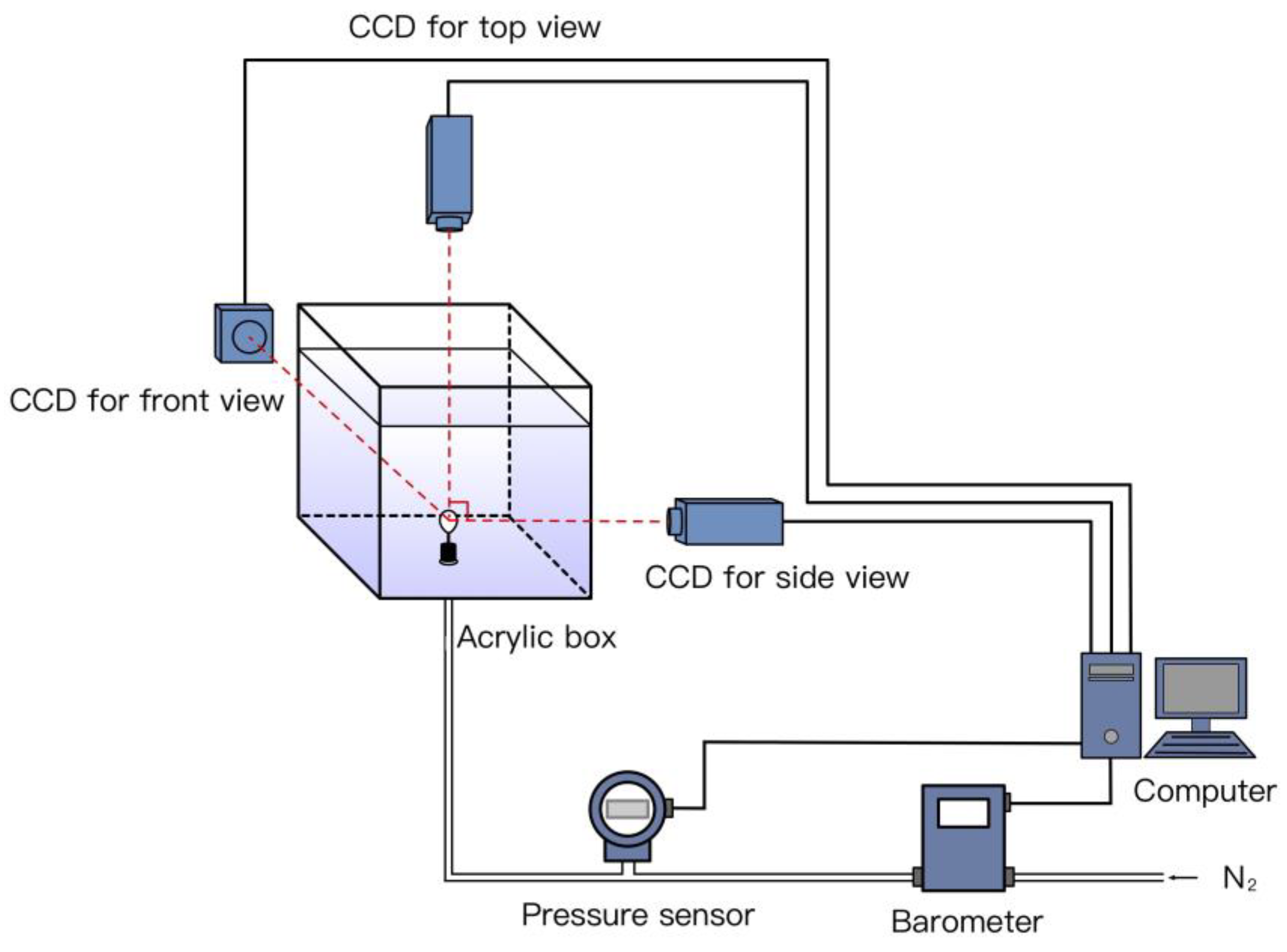
2.1. Experimental Set-Up

The schematic of the image acquisition device is illustrated in Figure 1. Laponite RD transparent soil [28] was used as the supporting medium to maintain the suspension of a single bubble in the center of an acrylic box, the size of which was 100 × 100 × 150 mm³. Three digital cameras (Baumer VCXG-13M), all connected to a computer, were utilized simultaneously for the front view, side view, and top view. Each camera had a matrix of 1024 × 1280 pixels and the size of the pixel was 0.0048 mm. The diameter of sparger was 1 mm. The distance between the front view camera and the center of the box was 463.0 mm, while the distance between the side view camera and the center of the box was 439.0 mm. Since the distance were much larger than experimental bubble diameter (less than 20 mm). Therefore, the distortion caused by light refraction between transparent soil and acrylic as well as the light refraction between acrylic and air was negligible. Two LED panels were placed behind the acrylic box to ensure sufficient illumination, which could reduce the significant errors in the bubble size measurement. Since the wall influence, which caused bubble asymmetry was uniform in cuboid acrylic box, the front view was similar to the side view and the top view resembled being circular.

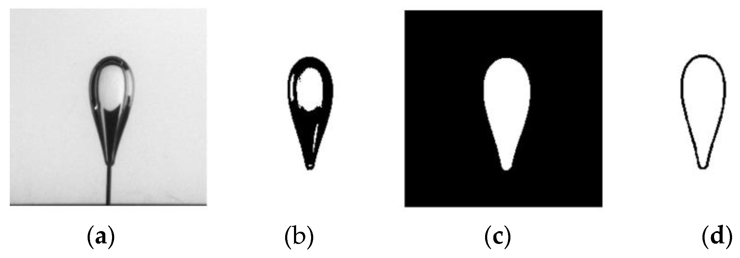
2.2. Image Processing and Camera Calibration

Images were processed by using MATLAB R2015a to obtain the bubble projection contours during the growth. The key result is shown in Figure 2. Figure 2a is one of the images taken by left view bubble in our experiment in Section 4.2. Figure 2b shows the image after dividing by a background image, which was without bubble, to enhance the contract and then binarizating with a threshold on the gray levels. From Figure 2c, we can notice that the holes are filled and noises are eliminated effectively. Bubble projection contours were detected by edge extraction method, as shown in Figure 2d.

After image processing, a calibrated chessboard was placed inside the acrylic box to determine the intrinsic parameters of cameras. According to the perspective of Zhang et al. and the application of their methods [29,30], the front and side camera parameters could be calculated, whose results were shown in

Table 1. The calibration parameters of front camera (pixel).

Calibration Parameters	Calibration Results
[$f_{11}$,$f_{21}$]	[2618.40929 2663.82735]
γ	[0.00000]
kc	[0.33266 −0.52175 0.07873 0.08099 0.00000]

and

Table 2. The calibration parameters of side camera (pixel).

Calibration Parameters	Calibration Results
[$f_{12}$,$f_{22}$]	[2702.94005 2677.29985]
γ	[0.00000]
kc	[0.13499 −0.35469 0.00509 −0.07338 0.00000]

, separately. According to the ideal pinhole model, the magnification factors are determined then for front camera (0.177 mm pixel⁻¹) and for side camera (0.171 mm pixel⁻¹). Because the top view camera was only used to extract the azimuth angle, which cannot be effected by magnifying, therefore it did not need to be calibrated.

where, f_ij is the calibrated focal length in pixels, subscript character i = 1,2 representing horizontal direction and vertical direction of pictures respectively while subscript character j = 1,2 representing front camera and side camera, respectively. γ is the skew coefficient defining the angle between the x and y pixel axes, k_c is the image distortion coefficients (radial and tangential distortions).

The calibrated focal length was slightly different from the data provided from manufacturer that the camera was equipped with lens of focal distance 12 mm. There are probably two main reasons causing this unexpectedly disparity. On the one hand, ideal pinhole image model was adopted in camera calibration process, assuming focal length was definite. However, the real cameras had much more complex construction. On the other hand, different locations and positions of the calibration chessboard can result in variant calibration results. Thus, calibrating results change with distances and postures. Therefore, in order to receive a more satisfying calibration result, each step of calibration should be done exactly and carefully. Besides, the high quality of calibration chessboard, appropriate illumination conditions, and suitable camera postures should also be taken into consideration.

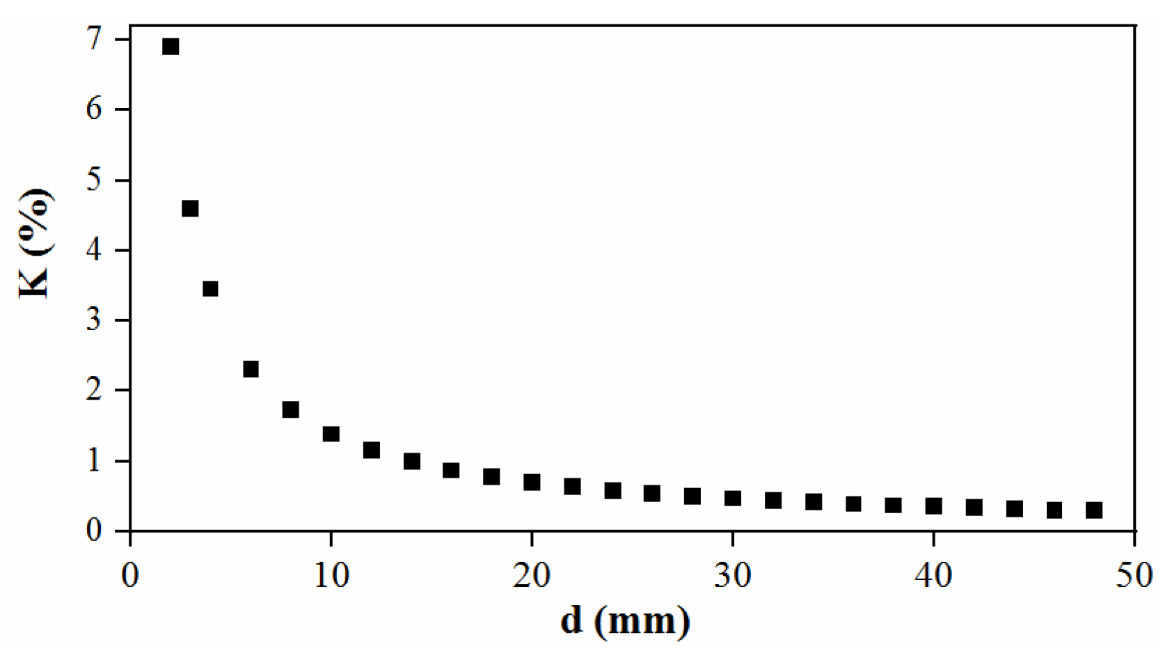
2.3. Measurement Accuracy

All steps of visualization produced uncertainties. First, high precision monox calibration chessboard was used to improve the measurement accuracy, the accuracy reached $\pm 0.01$ mm. Then, in order to eliminate the error produced by limited calibration pictures, this paper considers 30 different calibration postures as plentiful enough. We can easily know that one pixel created an measurement error of 0.0048 mm. Thus, the errors of hole filling as well as edge extraction could be measured and each of them exerted a negligible 0.1% on the measurement bubble length, as background division and binarization. Further, both front and side cameras induced uncertainty of local length through camera calibration process, which was [37.48217, 40.70242] and [56.57221, 64.13330] in pixels. Hence, the calibration errors in x and y pixel axes cold be calculated, respectively. In this way, the uncertainty on the measurement of bubble diameter was accumulated. According to the propagation law of errors:

$$m_d=\sqrt{\mathrm{mean}\left[{\displaystyle \sum _{i,j=1,2}\left({\left(\frac{1}{f_{ij}\cdot px}\right)}^2\cdot m_D^2+{\left(-\frac{D_j}{f_{ij}^2\cdot p{x}^2}\right)}^2\cdot m_{fij}^2+{\left(\frac{D_j}{f_{ij}\cdot px}\right)}^2\cdot m_c^2\right)}\right]}$$

(1)

where, m_d is the objective mean square error of bubble diameter, D_j is the distance between the cameras and the center of the box, and was measured by standard ruler. Therefore, the mean square error m_D was $\pm 1$ mm on the basis of ruler precision, m_f is the calibration mean square errors, px is the length of a pixel, m_c is the precision of calibration chessboard. Thus, after all the above operations, the measurement uncertainty on bubble diameter during camera calibration and image processing was estimated to be $\pm 0.46$ mm. The mean square error of spherical bubble volume can be deduced roughly as following:

$$m_V=\frac{\pi }{2}{d}^2\left|m_d^{}\right|$$

(2)

where, m_V is the objective mean square error of bubble volume, of which the measurement is the uncertainty evolution of bubble geometrical characteristics. Then the relative mean square error (K) could be written as:

$$K=\left|m_V^{}\right|/V_b$$

(3)

where, V_b is the volume of spherical bubbles. It can be seen in Figure 3 that K was the decreasing function of bubble diameter. With the bubble growth, the K met a relative stable level and the measurement accuracy increased. Pleased results (given the expected threshold K≦3%) could be met in the interval [4, +∞], which was quite acceptable in our experiments, where most of the bubble diameters were in this interval.

3. 3D Bubble Reconstruction

3.1. Modified Stacking Ellipse Method

The method in this paper proposed here included four steps as illustrated in Figure 4. The first step was to extract the projected contour of the bubble in three orthographic images, and the second step corrected the posture of the projected contour to make the c-axis (or z-axis) in the front view and the side view vertical or horizontal; the third step was also supposed to calculate the dimensionless major semi-axis (a₀) and minor semi-axis (b₀) of the horizontal elliptical cross-section by utilizing the projection relationship and the geometric information; the fourth step divided the bubble into n layers along the height direction (c-axis) and calculated the major semi-axis (a_i) and the minor semi-axis (b_i) of each horizontal ellipse slice. Finally, all the ellipse slices were stacked to form a 3D bubble shape.

3.2. Bubble Posture Correction

Bubble posture correction was the pre-work of the method proposed in this paper. There were two major purposes to carry out this step. On the one hand, based on the rotation conditions and geometric information of front contour and side contour around x-axis and y-axis, the posture correction improved the measurement accuracy of the azimuth angle around z-axis. On the other hand, the posture correction, which used the spatial rotation angles of bubble to correct their projection contours, properly reduced the measurement error causing by rotation. Figure 5 illustrates the schematic diagram of posture correction. Since the image processing steps of the front view are similar to those of the side view, as an example, the following statements are used to explain the steps of posture correction for the front view. In the following expressions, F, S, and T indicate the front view, side view, and top view, respectively.

The implementation details of bubble posture correction were shown in Figure 5. We considered images of sample No. 7 (As shown in the bubble examples in Section 4.1) to be the example. Firstly, the projected contours were extracted using image processing software MATLAB R2015a. Axis A was assumed to be the shorter axis, which is perpendicular to the longer axis, i.e., axis B. Moreover, the angle between axis A and the vertical direction, i.e., θ_F, was considered to be in the range of 0–90° (0° ≤ θ_F ≤ 90°). When θ_F is smaller than 45°, the projected contour of the top view of the bubble is mainly affected by the length of axis B, so axis A is rotated to the vertical direction; on the other hand, when θ_F is greater than 45°, the projected contour of the top view of the bubble is mostly affected by axis A, so axis A is rotated to the horizontal direction. The rotation formula is given by:

$$\left(\begin{array}{c}{x}_F^{\prime }\\ z_F^{\prime }\end{array}\right)=\left(\begin{array}{cc}\cos {\theta }_F& \sin {\theta }_F\\ -\sin {\theta }_F& \cos {\theta }_F\end{array}\right)\left(\begin{array}{c}{x}_F\\ z_F\end{array}\right)$$

(4)

where, (x_F, z_F) and ($x_F^{\prime }$, $z_F^{\prime }$) represent the coordinates of the bubble projection contour before rotation and after rotation, respectively; θ_F is the angle of rotation. Then, the magnification factor of the front view is calculated by:

$${\gamma }_F={s_F/S}_F$$

(5)

where, γ_F is the magnification factor of the front view; S_F and s_F represent the maximum width of the front image and that of the corrected front image, respectively. Meanwhile, the coincident steps were repeated to correct the projected contour of the side image, and the magnification factor of the side view (γ_S) was then figured.

Finally, in order to make the bubble contours conform to physical and geometric relationship, the top projection contour needed to be corrected using the magnification of the front view and side view as follows:

$$\left(\begin{array}{c}{x}_T^{\prime }\\ y_T^{\prime }\end{array}\right)=\left(\begin{array}{cc}{x}_T& 0\\ 0& y_T\end{array}\right)\left(\begin{array}{c}{\gamma }_F\\ {\gamma }_S\end{array}\right)$$

(6)

where, (x_T, y_T) are the coordinates of the uncorrected top view image, and ($x_T^{\prime }$, $y_T^{\prime }$) denote the coordinates of the corrected top view image. After the top view image was corrected, the angle between the long axis (or the short axis) and the horizontal direction was extracted and that was regarded as the azimuth angle (β_T).

3.3. Calculating Parameters of Horizontal Ellipse Slices

Since the dimension of the single bubble is much smaller than the distance between the camera and the bubble, it can be reasonable to assume that the incident light is parallel light, so the bubble is evenly divided into n pieces of ellipse slices along the height direction. Further, both of the azimuth angle (β_T) and the projection parameter, α (α_F or α_S), of the ellipse slices were assumed to be constant at each layer. The major and minor semi-axes of the ith layer of the ellipse at a height of H_i were indicated by a_i and bi, respectively, and the projection widths in the front and side views were denoted by l_Fi and l_Si, respectively (Figure 6). The equation of the ith layer of the ellipse projected onto the top view can be written by:

$$A_i{x}^2+B_i{y}^2+C_{i}xy=1$$

(7)

where, $A_i=\left(\frac{{\cos }^2{\beta }_T}{a_i^2}+\frac{{\sin }^2{\beta }_T}{b_i^2}\right)$, $B_i=\left(\frac{{\sin }^2{\beta }_T}{a_i^2}+\frac{{\cos }^2{\beta }_T}{b_i^2}\right)$, and $C_i=2\left(\frac{1}{a_i^2}-\frac{1}{b_i^2}\right)\cos {\beta }_T\sin {\beta }_T$.

Two tangent points are derived from the two tangent lines parallel with the x-axis on layer i, and the chord length of the line passing through the two tangent points and the ellipse is equal to the width of projection onto the side view (l_Si) as shown in Figure 6. The formula for l_Si is expressed as:

$$l_{Si}=\frac{2\tan {\alpha }_S}{\sqrt{A_i+B_i{\tan }_{}^2{\alpha }_S+C_i\tan {\alpha }_S}}$$

(8)

where, ${\alpha }_S$ is a projection parameter associated with the angle between the chord length and horizontal line. By rearranging, these parameters can be related as follows:

$$\frac{1}{l_{Si}^2}=\frac{c_1^2}{a_i^2}+\frac{c_1^2}{b_i^2}$$

(9)

where, $c_1=\frac{\cos {\beta }_T+\sin {\beta }_T\tan {\alpha }_S}{2\tan {\alpha }_S}$ and $c_2=\frac{\sin {\beta }_T-\cos {\beta }_T\tan {\alpha }_S}{2\tan {\alpha }_S}$.

By rearranging Equation (9) into a dimensionless equation, where $a_0=\frac{a_i}{l_{Si}}$ and $b_0=\frac{b_i}{l_{Si}}$, one may obtain:

$$\frac{c_1^2}{a_0^2}+\frac{c_2^2}{b_0^2}=1$$

(10)

The tangent coordinates of the tangent line, the slope of which is zero since it is parallel with the x-axis, are defined by (x, x tan α_S), where:

$$\frac{2A_i+C_i\tan {\alpha }_S}{2B_i\tan {\alpha }_S+C_i}=0$$

(11)

Equation (11) could be simplified as follows:

$$\frac{b_i}{a_i}=\frac{b_0}{a_0}=c_3$$

(12)

where, $c_3=\sqrt{\frac{\cos {\beta }_T\sin {\beta }_T\tan {\alpha }_S-{\sin }^2{\beta }_T}{\cos {\beta }_T\sin {\beta }_T\tan {\alpha }_S+{\cos }^2{\beta }_T}}$.

By combining Equations (10) and (12), one can obtain:

$$\{\begin{array}{c}{a}_0=\frac{1}{2}\sqrt{\frac{\cos ({\alpha }_S-{\beta }_T)}{\sin {\alpha }_S\sin {\beta }_T}}\\ b_0=\frac{1}{2}\sqrt{\frac{\sin ({\alpha }_S-{\beta }_T)}{\sin {\alpha }_S\cos {\beta }_T}}\end{array}$$

(13)

Equation (13) shows that the dimensionless parameters a₀ and b₀ are only associated with the azimuth angle (β_T), so the projection parameter (α_S) of an arbitrary ellipse slice is constant. Both the long semi-axis (a_i) and short semi-axis (b_i) of the ellipse slice in the ith layer can be calculated by the following formula:

$$\{\begin{array}{c}{a}_i=a_0\cdot l_{Si}\\ b_i=b_0\cdot l_{Si}\end{array}$$

(14)

Using the same procedure, similar results can also be obtained by using the projection width of the front view, and the corresponding dimensionless parameters of the ellipse can be calculated as:

$$\{\begin{array}{c}{a}_0=\frac{1}{2}\sqrt{\frac{\cos ({\alpha }_F-{\beta }_T)}{\cos {\alpha }_F\cos {\beta }_T}}\\ b_0=\frac{1}{2}\sqrt{\frac{-\sin ({\alpha }_F-{\beta }_T)}{\cos {\alpha }_F\sin {\beta }_T}}\end{array}$$

(15)

The long semi-axis (a_i) and short semi-axis (b_i) in layer i are defined using the following equation:

$$\{\begin{array}{c}{a}_i=a_0\cdot l_{Fi}\\ b_i=b_0\cdot l_{Fi}\end{array}$$

(16)

All the ellipse slices were then stacked to form the 3D shape of the single bubble after traversing each layer of the ellipse slice. It is worth noting that when β_T approached 90° inseparably, the solutions to Equations (13) and (15) were not practical in the reconstruction process under these conditions; therefore, it is reasonable to assume that both axes of each ellipse slice are equal to the corresponding projection width to avoid the odd points of Equations (13) and (15).

4. Benchmark with Synthetic Bubbles

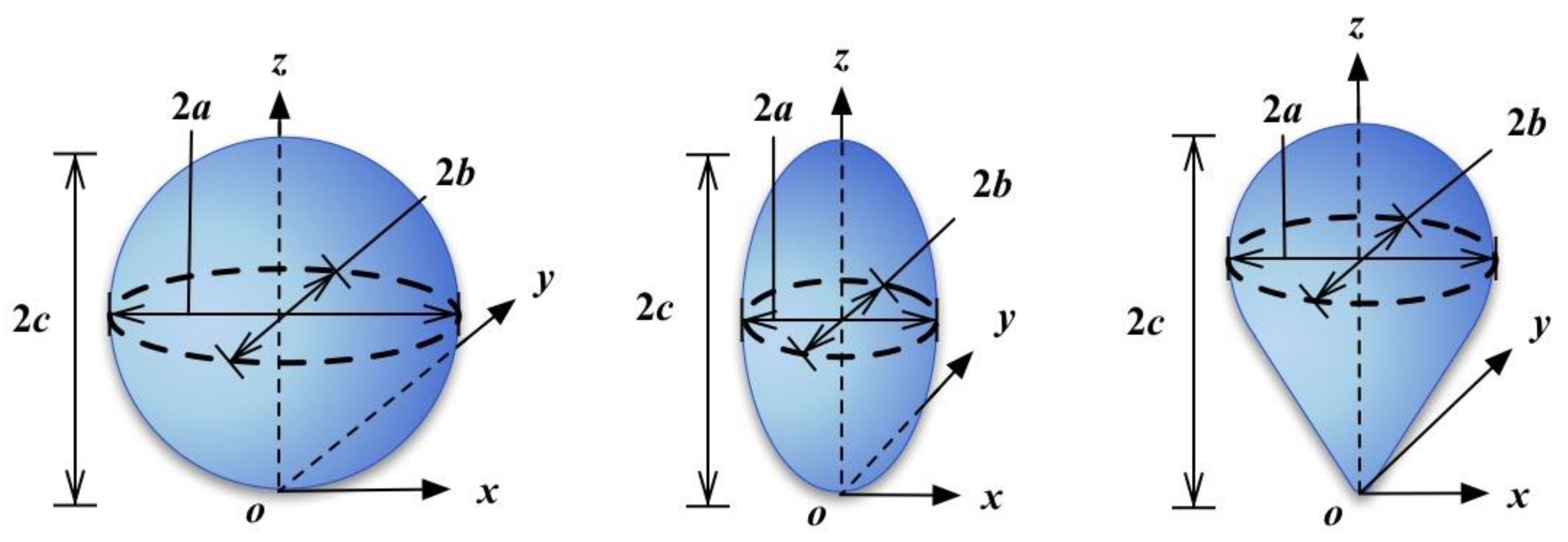
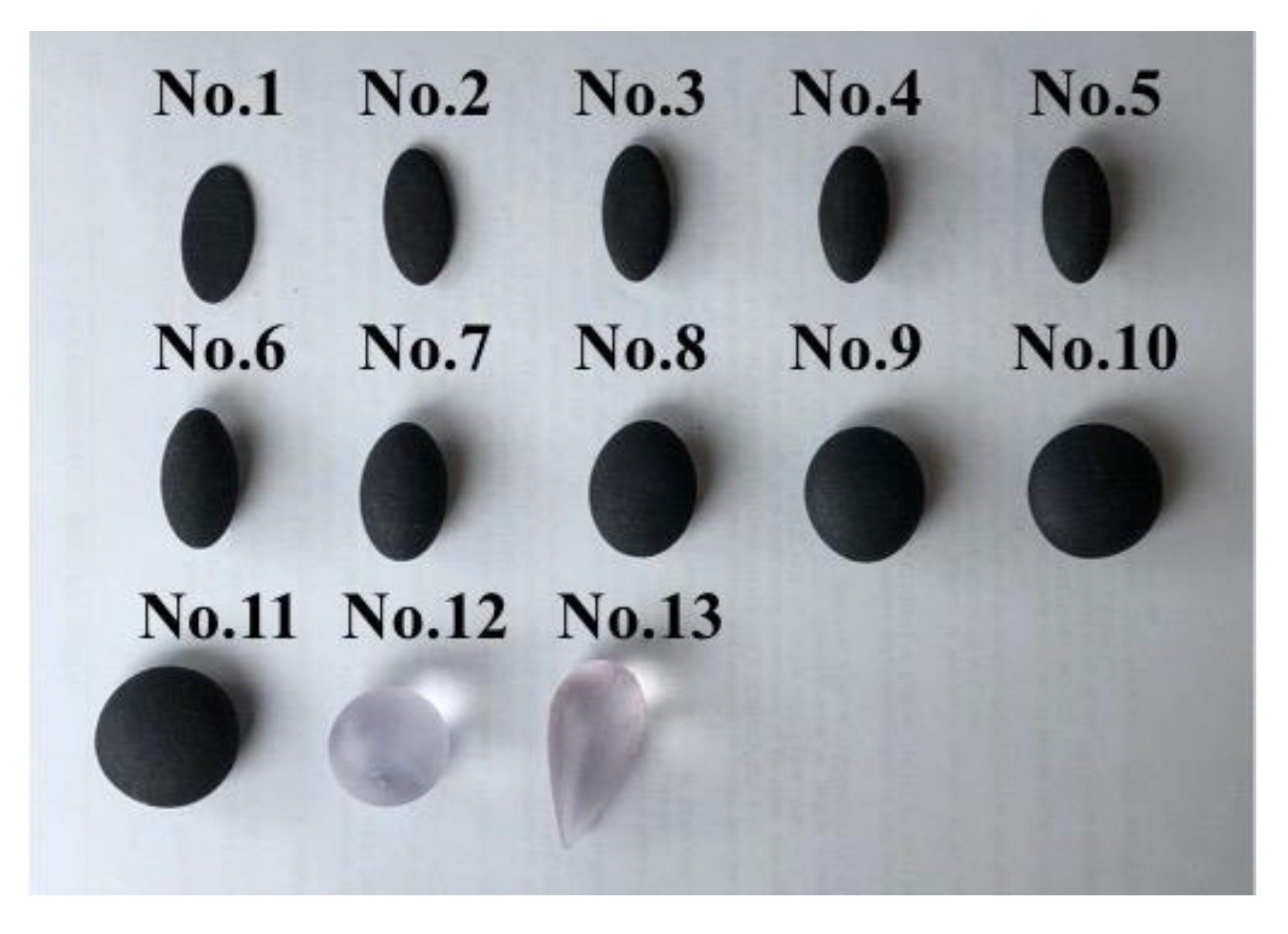
4.1. Bubble Samples

Many studies used bubble-like objects to test the accuracy of reconstruction [18,23]. Therefore, three different types of bubble-like object (hereinafter referred to as bubble) were produced using 3D printing technology as displayed in Figure 7, to evaluate the measurement accuracy of several reconstruction methods discussed above. The first type was a sphere, where all the semi-axes have equal lengths, i.e., a = b = c; this type is generally used in ideal situations [31,32]. The second type was an ellipsoid, in which at least two of the three semi-axes (a, b, and c) were unequal; this type is also suitable for describing the bubble in a shear flow [33,34]. The third type resembled an inverted teardrop, which is mostly developed in viscose or shear thinning fluids [1,4]. Since the finite acrylic box existed wall influence, which led to uncertainties and different a, b, and c values, a series of objects with identical a and c but different b values were generated. An inverted droplet was produced using equal values of a and b, denoting a circular horizontal cross-section. Furthermore, the accuracy of 3D printing was $\pm 0.01$ mm. Hence, the total measurement accuracy calculated by Equation (1) was $\pm 0.46$ mm. The accuracy of volume, tested by the densimeter AU-300PM, was $\pm 1$ mm³. The locations of cameras were stationary during experiments. Thus, the bubble parameters can be measured (

Table 3. The parameters of the different produced bubbles.

Bubble Shape	Sample No.	2a (mm)	2b (mm)	2c (mm)	Volume (mm3)
Ellipsoid	1	20	2	10	223
	2	20	3	10	316
	3	20	5	10	549
	4	20	7	10	784
	5	20	9	10	946
	6	20	11	10	1113
	7	20	13	10	1321
	8	20	15	10	1623
	9	20	17	10	1825
	10	20	19	10	1997
	11	20	20	10	2079
Sphere	12	16	16	16	2141
Inverted teardrop	13	15	15	32	2522

) and the objects are shown in Figure 8.

4.2. Effects of Posture Correction

The bubble volume was used to measure the accuracy of the reconstruction results. The difference between the calculated volume and the actual volume in the form of mean relative error (MRE) was calculated during experiments. The standard deviation of the calculated results was represented by error bars. All the examples were tested three times and the rotation angles around x-axis, y-axis, and z-axis of each test case were generated randomly.

Figure 9 compares the accuracy of the reconstruction methods (in the form of MRE) with/without posture correction, where the sphere (sample No. 12), ellipsoid (sample No. 7), and inverted teardrop (sample No. 13) are analyzed using the methods in this paper, Fujiwara et al. [21], and Bian et al. [20]. Since the spheres have an equivalent length in whichever direction, posture correction does not theoretically influence the reconstruction, leading to slight distinction between the corrected and uncorrected data. On the other hand, the ellipsoids reflect the degree of deformation in the horizontal direction, while the inverted teardrops show the degree of deformation in the vertical direction. Therefore, by comparing the data on the ellipsoids and the inverted teardrops, it can logically be found that posture correction significantly enhances the reconstruction accuracy of the method in this paper, but the effects on methods in Fujiwara et al. [21] and Bian et al. [20] are slight. This indicates that the posture correction is undoubtedly required in our method for the reconstruction of bubbles having serious deformation.

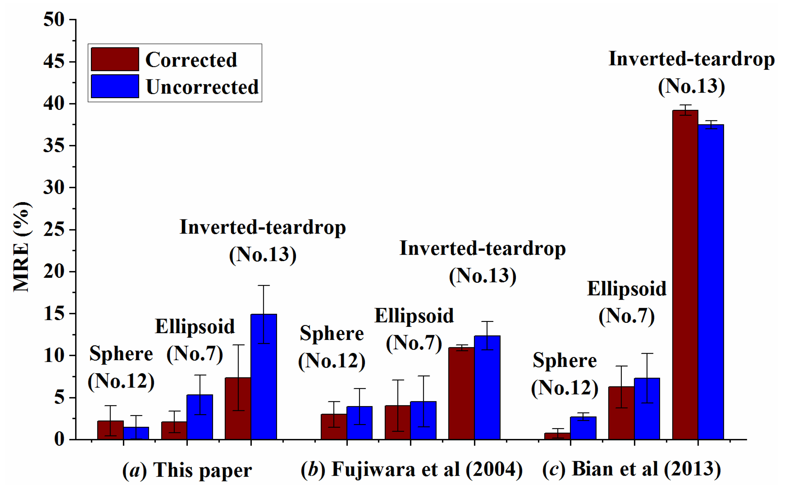
4.3. Effects of Different Shapes

It can be seen in Figure 10 that the MRE calculated for the three methods is approximately less than 3% when the bubble resembles a sphere, which indicates that the three methods can well reconstruct spherical bubbles. Nevertheless, when the bubble is deformed in the horizontal direction, such as ellipsoidal bubbles, the accuracy of the reconstruction methods changes progressively in the order this paper > Fujiwara et al. [21] > Bian et al. [20], that is, the modified stacked ellipse method leads to the smallest mean relative error in reconstructing the bubble. In fact, since the method in Fujiwara et al. [21] utilizes the projection width onto the front and side views as the long and short axes of the ellipse on each ellipse slice respectively, when the major axis of the ellipse is not equal to the projection width, that is, β_T is deviated from either 0 or 90°, the method in Fujiwara et al. [21] leads to a larger error in reconstructing the bubble (this phenomenon could also been seen in Section 4.5). Furthermore, the assumption of Bian et al. [20] that a bubble has a minimum rotation angle around z-axis was overturned because the azimuth angle β_T always exists, and the bubble’s highest point is not always located at the z-axis. Therefore, Bian et al. [20] overestimate the bubble, especially when the bubble is not elliptical. In this way, the method in Bian et al. [20] leads to a greater error in reconstructing the bubble compared with the method in Fujiwara et al. [21]. When the deformation of the bubble is increased in the vertical direction, that is, the bubble has an inverted-teardrop shape. The method in this paper shows a surprising degree of accuracy, and the method in Fujiwara et al. [21] is also far superior to the method in Bian et al. [20], which is attributed to the fact that the methods in this paper and Fujiwara et al. [21] stack ellipse slices along the vertical direction, causing a minimal impact on the reconstruction accuracy when vertical deformation increases. The method in Bian et al. [20] assumes that the vertical projection is oval, which leads to an extremely large MRE in reconstructing an inverted teardrop-shaped bubble.

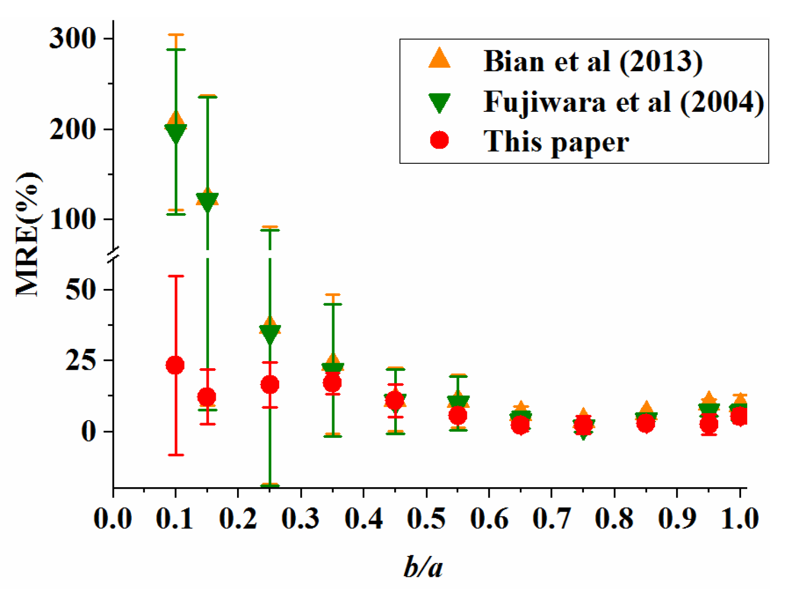
4.4. Effects of Deformation

The above analysis revealed that the degree of bubble deformation has a significant effect on the reconstruction accuracy. Therefore, the following ellipsoids (samples No. 1–11) were used as examples to analyze the influences of the horizontal deformation of the bubble, in terms of the ratio of the vertical axis to the horizontal axis, i.e., (b/a), and the sphericity of the bubble on the accuracy of the reconstruction algorithms.

Figure 11 shows that the MRE values of the three methods are similar when the ratio of the vertical axis to the horizontal axis, (b/a), is greater than 0.5 and confirms that the method in this paper performs better than the two other methods with a reconstruction error smaller than 6%. Reducing the ratio of the vertical axis to the horizontal axis in the range of 0 to 0.5 increases the mean relative error obtained by the three methods. Moreover, the mean relative error in reconstructing the bubble by the method in this paper is not more than 24%, which denotes a satisfying degree of accuracy. Nonetheless, the accuracy of the method in Fujiwara et al. [21] is closely similar to that of the method in Bian et al. [20] since all the analyzed samples are standard ellipsoids, the vertical projection of which is oval. Therefore, the capability of the method in Fujiwara et al. [21] to resist vertical deformation does not give it an advantage over the method in Bian et al. [20] in this case.

Sphericity (s), as a parameter measuring the degree of deviation of an object from a sphere, is defined by:

$$s=S_s/S_o$$

(17)

where, S_S denotes the surface area of a sphere having the same volume as the object, and S_O stands for the surface area of the object.

Figure 12 demonstrates that the accuracy of the three methods in calculating the bubble volume, or rather reconstructing the bubble, is not much different when the sphericity is greater than 0.90; however, the method in this paper is slightly more accurate than the two other methods.

Therefore, based on the above discussion, the method in this paper is more accurate and has better applicability when the bubble is horizontally or vertically deformed.

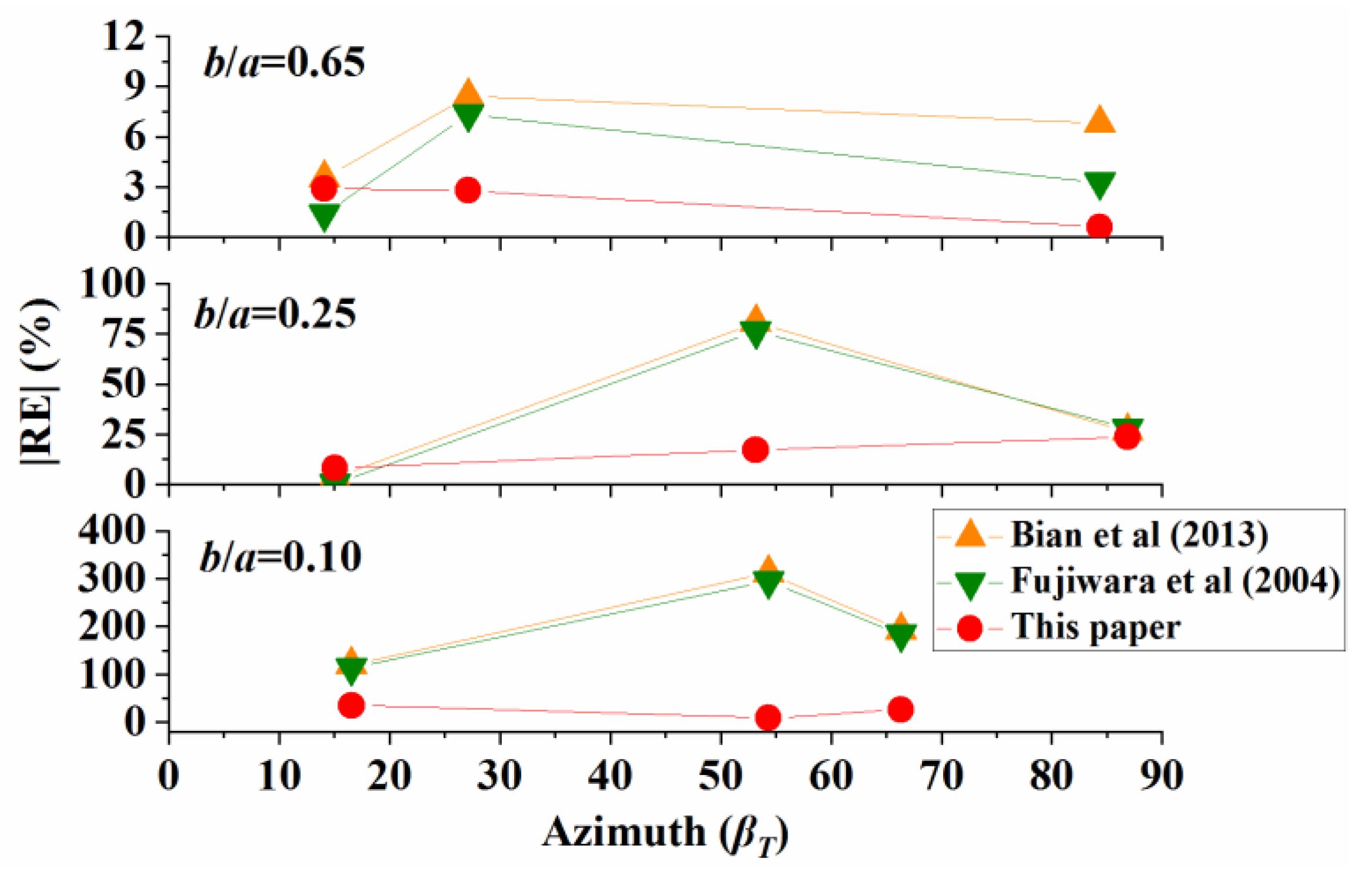
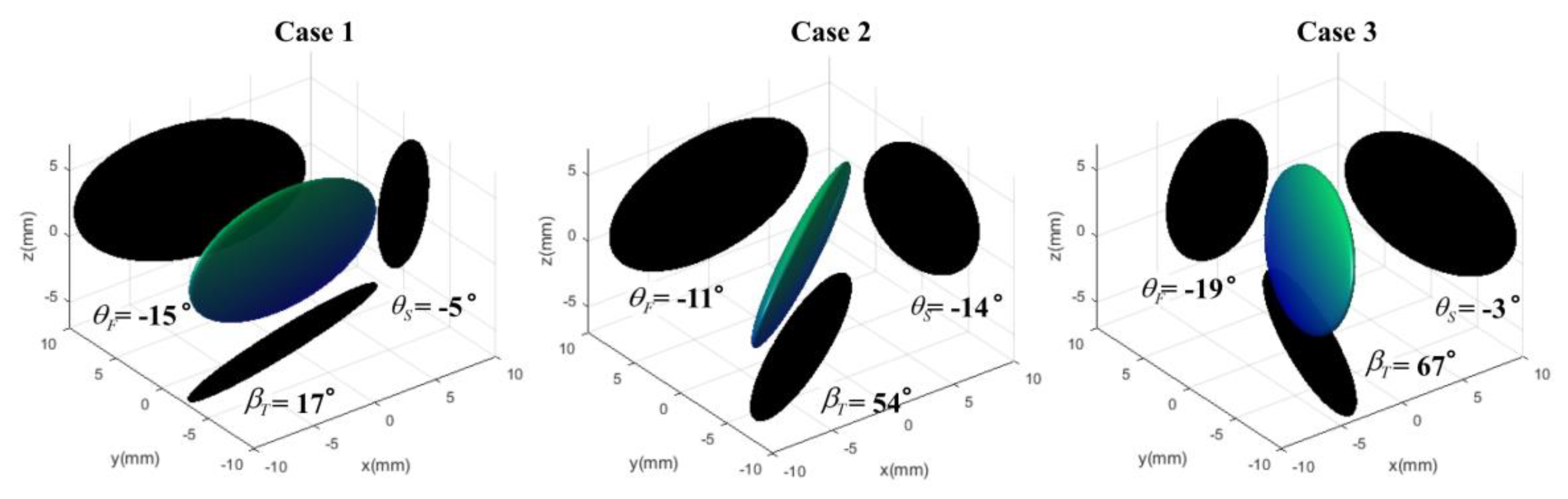
4.5. Effects of Azimuth Angle

The effect of azimuth angle on the accuracy of the reconstruction methods is studied by reconstructing three ellipsoids (samples No. 1, 3, and 7), as delineated in Figure 13. The mean relative error in the bubble volume calculated by the three methods, which denotes the accuracy of the methods in reconstructing the bubble, is similar when the azimuth angle is close to either 0 or 90°. However, when the azimuth angle gradually deviates from either 0 or 90°, the mean relative errors calculated by both the method in Fujiwara et al. [21] and Bian et al. [20] are obviously larger than the MRE obtained by the method in this paper. Figure 13 shows the methods of Fujiwara et al. [21] and Bian et al. [20] were more sensitive to bubble shape and rotation angles. Besides, the method in this paper was more stable in measuring bubble volume. It is notable that the bubble shapes and rotation angles had little impact on the volume measurement accuracy using the method in this paper.

The ellipsoid (No.1) in 3rd graph of Figure 13 was visualized in Figure 14 as an example, with their corresponding projection images for front view, side view, and top view. As shown in case 1 to 3 of Figure 14, the projection contours always overstated the bubble size. If bubble rotated around z axis, the front view and side view projection contours would become much larger. The reconstruction methods based on Fujiwara et al. [21] and Bian et al. [20], by this token, would have larger uncertainties and unstable predictions. This scenario got significant when the azimuth angle was approximate to 45°.

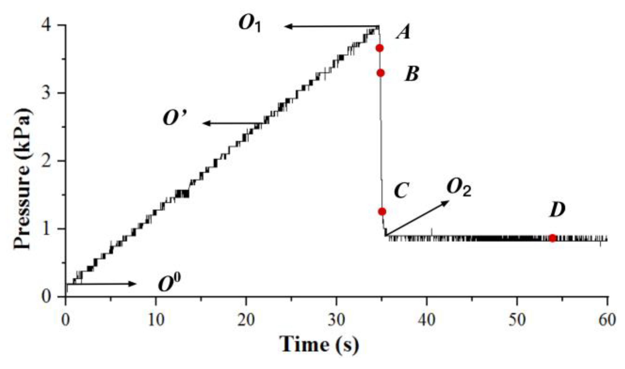
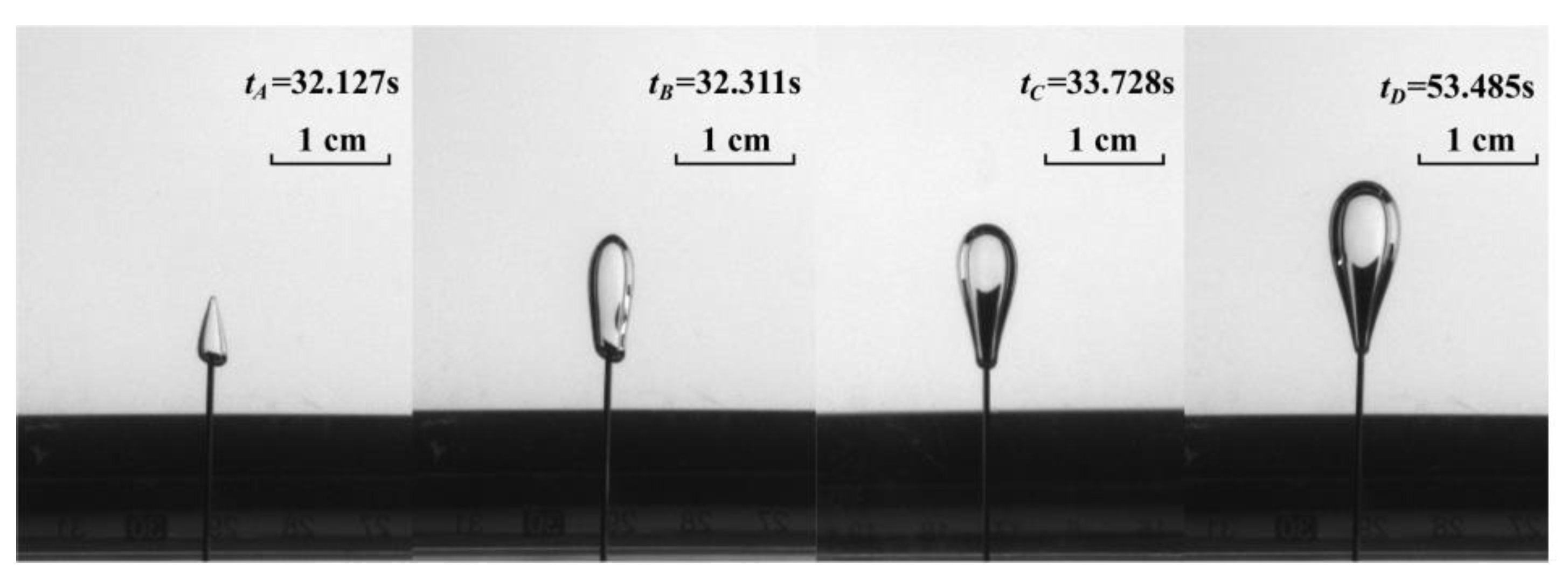
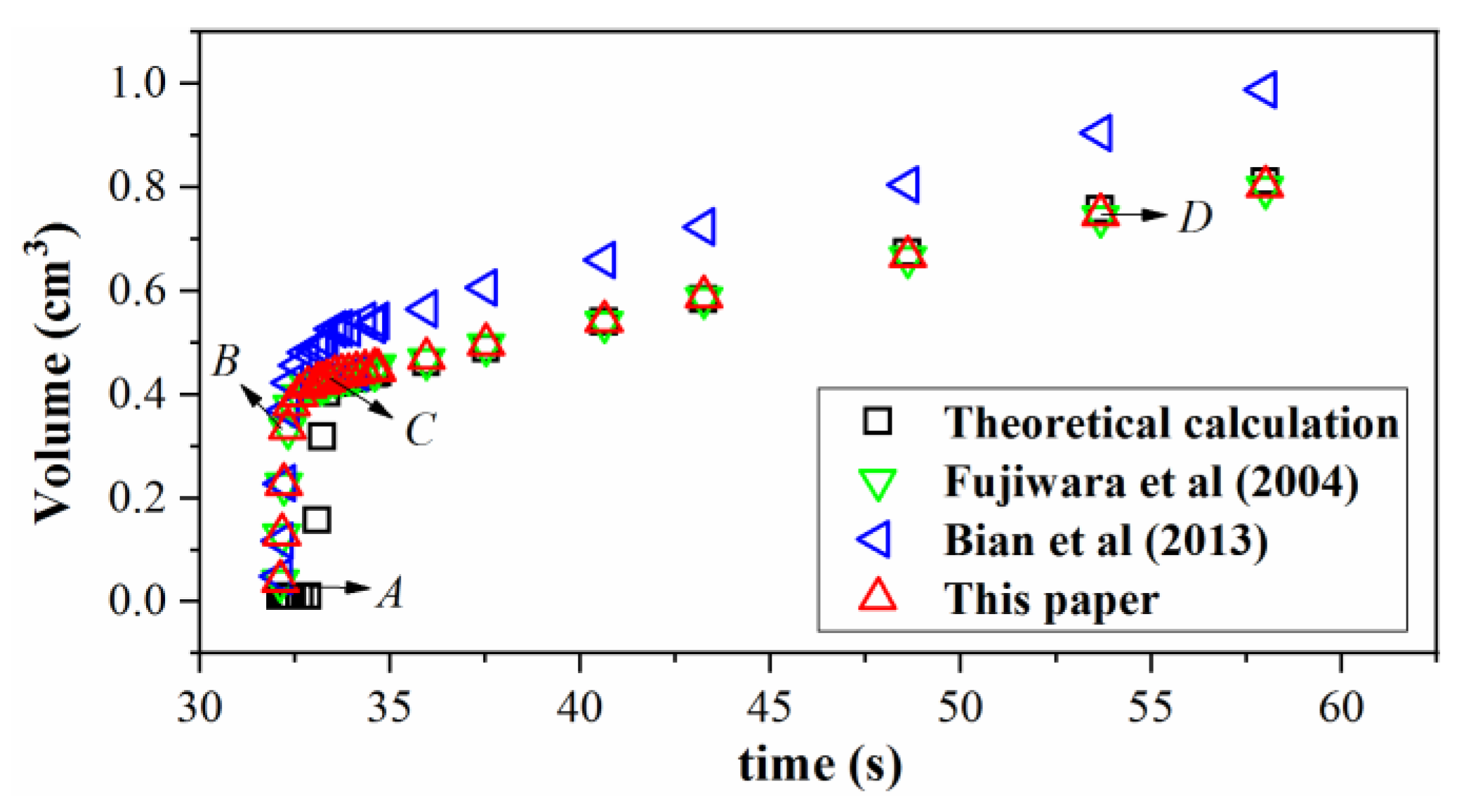
5. Verification by Gas Injection Test

To further verify the accuracy of the method in this paper, a gas injection test was conducted using the experimental apparatus in Section 2. During this experiment, the bubble images were taken by three cameras, the gas flow rate was set as 1 sccm, and the gas pressure was recorded by pressure sensor sequentially. As we can see in Figure 15, the pressure increased steadily until it met a peak, and then dropped ephemerally. After that, it maintains a stable horizontal level. The bubble appeared soon after the pressure reached peak and it grew during the period of pressure drop and the stable pressure level. Images at four different time nodes (A–D) were stitched together to visualize the bubble growth.

The experimental bubble volumes were calculated by following steps based on Van der Waals (1873). The initial condition (point O₀) could be written as:

$$\left(P_0+\frac{n_0^{2}a}{V_{pipe}^2}\right)(V_{pipe}-n_{0}b)=n_{0}RT$$

(18)

where, P₀ is the initial pipe pressure, and the n₀ is initial mole numbers inside the pipe, V_pipe is the pipe volume. The Van der Waals parameters $a=0.1408 \mathrm{Pa}\cdot {\mathrm{m}}^6\cdot {\mathrm{mol}}^{-2}$, $b=3.912\times {10}^{-5} {\mathrm{m}}^5\cdot {\mathrm{mol}}^{-1}$, and the ideal gas constant $R=8.31441\pm 0.00026 \mathrm{J}/(\mathrm{mol}\cdot \mathrm{K})$. The thermodynamic temperature K inside the laboratory was 288 K. For a moment (point O’) where the bubble had not generated:

$$\left(P^{\prime }+\frac{{(n_0+n^{\prime })}^{2}a}{V_{pipe}^2}\right)(V_{pipe}-(n_0^{}+n^{\prime })b)=(n_0+n^{\prime })RT$$

(19)

By combining Equations (18) and (19), both P₀ and n₀ were solved. For the period of pressure drop (point O₁ to O₂) in Figure 15:

$$\left(P_1+\frac{{(n_0^{}+n_2)}^{2}a}{V_{pipe}^2}\right)(V_{pipe}-(n_0^{}+n_2)b)=\left(P_2+\frac{{(n_0^{}+n_2)}^{2}a}{{(V_{pipe}^{}+V_{b2})}^2}\right)(V_{pipe}+V_{b2}-(n_0^{}+n_2)b)$$

(20)

where, P₁ is the beginning pressure of pressure drop, and P₂ is the ending pressure of pressure drop, V_b2 is the calculated bubble volume at the point O₂, n₂ is the mole numbers at the point O₂:

$$n_2=q{t}_2/22.4$$

(21)

Then, the bubble volume (V_b) after O₂ are:

$$V_b=q\left(t_x-t_2\right)+V_{b2}$$

(22)

where, t_x is the experimental time. A series of experiment pictures (corresponding to points A—D respectively in Figure 15) were taken based on the setup, some of which were shown as example in Figure 16. To further testify the accuracy of the method proposed above, they were reconstructed in Figure 17. It can be seen that the bubbles developed vertically and the projections for horizontal direction were analogue. The bubble shape was close to cone at the beginning, and then developed to ellipsoid quickly. The tip of the cusp emerged as bubble volume increased, and eventually evolved into shape of inverted teardrop.

The bubble volume measured by the methods in this paper, in Fujiwara et al. [21] and in Bian et al. [20], are shown in Figure 18. The construction results of the method in this paper fits well with the theoretical results and the MRE of bubble volume later O₂, which was 1.79%. Similarly, the construction results of the method in Fujiwara et al. [21] also fits the theoretical results perfectly, and the MRE of bubble volume later O₂ was 1.74%. The construction results of the method in Bian et al. [20] fits the theoretical results at the beginning; however, the error arose as time went by. In the method of Bian et al. [20], the MRE of bubble volume was 21.2%. As observed in gas injection test, the horizontal deformation of bubble was negligible due to the same effect of wall effect. Therefore, the construction results in this paper were almost the same as that in Fujiwara et al. [21]. Furthermore,, the vertical shape of bubble developed from ellipses to inverted-droplet, causing the construction accuracy high firstly and reduced later. It indicated that the method in this paper per have credible consistency with experimental results where bubbles had larger vertical deformation and little horizontal deformation.

Nonetheless, the method in this paper met relatively large reconstruction error during the pressure period [O₁, O₂]. The most possible reason was that it too quickly declined the pressure during pressure period [O₁, O₂] in a small time interval to the pressure sensor to record the changes. However, errors seemed to decrease in later period [O₂, end] where the time intervals become lager.

6. Conclusions

In the present work, we developed a precise method based on orthographic images to reconstruct a 3D bubble shape of a single bubble, which is elliptical in the horizontal direction and has an arbitrary shape in the vertical direction. The proposed reconstruction method demonstrated a surprising degree of accuracy compared with the methods in Fujiwara et al. [21] and Bian et al. [20], and its superiority was notable when the bubble deformation was increased.

The method in this paper differed from Fujiwara et al. [21] in two points. Firstly, the posture correction reduced the tilt problem caused by bubble oscillation. Second, the projection relationship and the geometric information were used to calculate the major and minor semi-axes of each horizontal ellipse slices. Therefore, instead of using the projection width directly, the method in this paper reduced the negative impact of horizontal deformation and azimuth angle on the reconstruction accuracy.

According to the above discussion, the following conclusions can be drawn:

(1)

The posture correction helps to improve the reconstruction accuracy in this paper, especially for the bubble with a horizontal cross-section remarkably deviating from a circle.

(2)

The dimensionless parameters of an ellipse in horizontal section (major and minor semi-axes) are independent of the projection width. By using the dimensionless elliptic parameters, the actual major and minor semi-axes of the horizontal elliptical section of each layer can be quickly calculated.

(3)

The method in Bian et al. [20] is more suitable for reconstructing a bubble similar to an ellipsoid because both of the horizontal and vertical deformations inversely impact its accuracy. The vertical deformation has a little influence on the method in Fujiwara et al. [21], but the horizontal deformation contributes significantly to its accuracy, especially when the ratio of the vertical axis to the horizontal axis is smaller than 0.5 or when the azimuth angle deviates greatly from either 0 or 90°.

(4)

The method in this paper successfully improves the flaws in methods in Bian et al. [20] and Fujiwara et al. [21]. The method in this paper can better reconstruct the bubble with severe horizontal deformation; in addition, similarly to the method in Fujiwara et al. [21], the vertical deformation has a negligible influence on the reconstruction accuracy of the method in this paper, leading to its higher practicality.

(5)

The two methods in Bian et al. [20] and Fujiwara et al. [21] are extremely sensitive to the orientation of the bubble since the azimuth angle of the horizontal elliptical slice strongly affects the reconstruction accuracy; however, it does not impact the method in this paper.

The bubble-shaped samples used in our experiments were considered to be regular bubbles since the bubbles generally representing a larger volume, less distortion, and a regular shape in Newtonian or non-Newtonian fluids with higher viscosity are similar to regular bubbles. Therefore, the reconstruction method developed herein is undoubtedly suitable for such a kind of bubbles. However, the application of the proposed method to reconstructing bubbles with a large horizontal and/or vertical distortion must be further validated. In this way, further exploration needs to be done to study the accuracy of this method when bubbles have both vertical and horizontal deformation. The algorithm should be sufficiently replenished on the problem that cameras are not ideal when perpendicular to each other.

References

1. Sattari, A.; Hanafizadeh, P. Bubble formation on submerged micrometer-sized nozzles in polymer solutions: An experimental investigation. Colloid. Surface. A. 2019, 564, 10–22. [Google Scholar] [CrossRef]
2. Deng, B.; Chin, R.J.; Tang, Y.; Jiang, C.; Lai, S.H. New Approach to Predict the Motion Characteristics of Single Bubbles in Still Water. Appl. Sci. 2019, 9, 3981. [Google Scholar] [CrossRef] [Green Version]
3. Clift, R.; Grace, J.R.; Weber, M.E. Bubbles, Drops, and Particles; Academic Press: New York, NY, USA, 2005. [Google Scholar]
4. Mirsandi, H.; Smit, W.J.; Kong, G.; Baltussen, M.W.; Peters, E.A.J.F.; Kuipers, J.A.M. Influence of wetting conditions on bubble formation from a submerged orifice. Exp. Fluids 2020, 61, 83. [Google Scholar] [CrossRef] [Green Version]
5. Zenit, R.; Feng, J.J. Hydrodynamic Interactions among Bubbles, Drops, and Particles in Non-Newtonian Liquids. Ann. Rev. Fluid Mech. 2018, 50, 505–534. [Google Scholar] [CrossRef]
6. Benzing, R.J.; Myers, J.E. Low frequency bubble formation at horizontal circular orifices. Ind. Eng. Chem. 1955, 47, 2087–2090. [Google Scholar] [CrossRef]
7. Fourest, T.; Laurens, J.; Deletombe, E.; Dupas, J.; Arrigoni, M. Analysis of bubbles dynamics created by Hydrodynamic Ram in confined geometries using the Rayleigh-Plesset equation. Int. J. Impact Eng. 2014, 73, 66–74. [Google Scholar] [CrossRef]
8. Wang, Z.; Qin, Y.; Zou, L. Analytical solutions of the Rayleigh-Plesset equation for N-dimensional spherical bubbles. Sci. China Phys. Mech. 2017, 60, 104721. [Google Scholar] [CrossRef]
9. Vafaei, S.; Wen, D. Bubble formation on a submerged micronozzle. J. Colloid Interf. Sci. 2010, 343, 291–297. [Google Scholar] [CrossRef]
10. Gharedaghi, H.; Dousti, A.; Eshraghi, J.; Hanafizadeh, P.; Ashjaee, M. A novel numerical approach for investigation of the gas bubble characteristics in stagnant liquid using Young-Laplace equation. Chem. Eng. Sci. 2017, 173, 37–48. [Google Scholar] [CrossRef]
11. Zhang, S.; Wang, S.P.; Zhang, A.M.; Cui, P. Numerical study on motion of the air-gun bubble based on boundary integral method. Ocean. Eng. 2018, 154, 70–80. [Google Scholar] [CrossRef]
12. Tian, Z.L.; Liu, Y.L.; Zhang, A.M.; Wang, S.P. Analysis of breaking and re-closure of a bubble near a free surface based on the Eulerian finite element method. Comput. Fluids 2018, 170, 41–52. [Google Scholar] [CrossRef]
13. Mukin, R.V. Bubble reconstruction method for wire-mesh sensors measurements. Exp. Fluids 2016, 57, 133. [Google Scholar] [CrossRef]
14. Wang, Q.; Jia, X.; Wang, M. Bubble mapping: Three-dimensional visualisation of gas-liquid flow regimes using electrical tomography. Meas. Sci. Technol. 2019, 30, 45303. [Google Scholar] [CrossRef]
15. Sun, J.; Zhang, H.; Li, J.; Zhou, Y.; Jia, D.; Liu, T. Hybrid spherical particle field measurement based on interference technology. Meas. Sci. Technol. 2017, 28, 35204. [Google Scholar] [CrossRef]
16. Boden, S.; Haghnegandar, M.; Hampel, U. Measurement of Taylor bubble shape in square channel by microfocus X-ray computed tomography for investigation of mass transfer. Flow Meas. Instrum. 2017, 53, 49–55. [Google Scholar] [CrossRef]
17. Jamaludin, J.; Rahim, R.A.; Rahim, H.A.; Rahiman, M.H.F.; Muji, S.Z.M.; Rohani, J.M. Charge coupled device based on optical tomography system in detecting air bubbles in crystal clear water. Flow Meas. Instrum. 2016, 50, 13–25. [Google Scholar] [CrossRef]
18. Lewandowski, B.; Ulbricht, M.; Krekel, G. An automated image analysing routine for estimation of equivalent diameter in high-speed image sequences with high accuracy and its validation. Exp. Therm. Fluid Sci. 2018, 98, 158–169. [Google Scholar] [CrossRef]
19. Wang, E.N.; Devasenathipathy, S.; Lin, H.; Hidrovo, C.H.; Santiago, J.G.; Goodson, K.E.; Kenny, T.W. A hybrid method for bubble geometry reconstruction in two-phase microchannels. Exp. Fluids 2006, 40, 847–858. [Google Scholar] [CrossRef]
20. Bian, Y.; Dong, F.; Zhang, W.; Wang, H.; Tan, C.; Zhang, Z. 3D reconstruction of single rising bubble in water using digital image processing and characteristic matrix. Particuology 2013, 11, 170–183. [Google Scholar] [CrossRef]
21. Fujiwara, A.; Danmoto, Y.; Hishida, K.; Maeda, M. Bubble deformation and flow structure measured by double shadow images and PIV/LIF. Exp. Fluids 2004, 36, 157–165. [Google Scholar] [CrossRef]
22. Zhang, T.; Qian, Y.; Yin, J.; Zhang, B.; Wang, D. Experimental study on 3D bubble shape evolution in swirl flow. Exp. Therm. Fluid Sci. 2019, 102, 368–375. [Google Scholar] [CrossRef]
23. Fu, Y.; Liu, Y. 3D bubble reconstruction using multiple cameras and space carving method. Meas. Sci. Technol. 2018, 29, 75206. [Google Scholar] [CrossRef]
24. Belden, J.; Ravela, S.; Truscott, T.T.; Techet, A.H. Three-dimensional bubble field resolution using synthetic aperture imaging: Application to a plunging jet. Exp. Fluids 2012, 53, 839–861. [Google Scholar] [CrossRef]
25. Masuk, A.U.M.; Salibindla, A.; Ni, R. A robust virtual-camera 3D shape reconstruction of deforming bubbles/droplets with additional physical constraints. Int. J. Multiphas. Flow 2019, 120, 103088. [Google Scholar] [CrossRef]
26. Di Nunno, F.; Alves Pereira, F.; de Marinis, G.; Di Felice, F.; Gargano, R.; Miozzi, M.; Granata, F. Deformation of Air Bubbles Near a Plunging Jet Using a Machine Learning Approach. Appl. Sci. 2020, 10, 3879. [Google Scholar] [CrossRef]
27. Wang, H.; Xu, H.; Pooneeth, V.; Gao, X. A Novel One-Camera-Five-Mirror Three-Dimensional Imaging Method for Reconstructing the Cavitation Bubble Cluster in a Water Hydraulic Valve. Appl. Sci. 2018, 8, 1783. [Google Scholar] [CrossRef] [Green Version]
28. Zhang, Y.; Hu, M.; Ye, T.; Chen, Y.; Zhou, Y. An experimental study on the rheological properties of laponite RD as a transparent soil. Geotech. Test. J. 2020, 43, 607–621. [Google Scholar] [CrossRef]
29. Zhang, Z.Y. A flexible new technique for camera calibration. IEEE Trans. Pattern Anal. Mach. Intell. 2000, 22, 1330–1334. [Google Scholar] [CrossRef] [Green Version]
30. Xue, T.; Qu, L.; Cao, Z.; Zhang, T. Three-dimensional feature parameters measurement of bubbles in gas-liquid two-phase flow based on virtual stereo vision. Flow Meas. Instrum. 2012, 27, 29–36. [Google Scholar] [CrossRef]
31. Supponen, O.; Obreschkow, D.; Kobel, P.; Dorsaz, N.; Farhat, M. Detailed experiments on weakly deformed cavitation bubbles. Exp. Fluids 2019, 60, 33. [Google Scholar] [CrossRef]
32. Hamaguchi, F.; Ando, K. Linear oscillation of gas bubbles in a viscoelastic material under ultrasound irradiation. Phys. Fluids 2015, 27, 113103. [Google Scholar] [CrossRef]
33. Okawa, T.; Ishida, T.; Kataoka, I.; Mori, M. Bubble rise characteristics after the departure from a nucleation site in vertical upflow boiling of subcooled water. Nucl. Eng. Des. 2005, 235, 1149–1161. [Google Scholar] [CrossRef]
34. Kong, G.; Mirsandi, H.; Buist, K.A.; Peters, E.A.J.F.; Baltussen, M.W.; Kuipers, J.A.M. Oscillation dynamics of a bubble rising in viscous liquid. Exp. Fluids 2019, 60, 130. [Google Scholar] [CrossRef] [Green Version]
Figure 1. Experimental set-up.
Applsci 10 05803 g001
Figure 2. Steps of image processing. (a) Initial image, (b) background division and binarization, (c) hole filling, (d) edge extraction.
Applsci 10 05803 g002
Figure 3. The relative mean square errors (K) vary with bubble diameters.
Applsci 10 05803 g003
Figure 4. A 3D schematic of the method proposed in this paper.
Applsci 10 05803 g004
Figure 5. A schematic of posture correction.
Applsci 10 05803 g005
Figure 6. Corrected orthographic images.
Applsci 10 05803 g006
Figure 7. Synthetic bubbles: from left to right, a sphere, an ellipsoid, and an inverted teardrop. The 2a, 2b, and 2c are three characteristic parameters that represent bubble shape. The axes 2a and 2b represents the two horizontal axes, while 2c represents the vertical axis.
Applsci 10 05803 g007
Figure 8. Images of the bubble samples.
Applsci 10 05803 g008
Figure 9. The effect of posture correction on the accuracy of the reconstruction methods.
Applsci 10 05803 g009
Figure 10. The accuracy of the reconstruction methods in reconstructing different shapes.
Applsci 10 05803 g010
Figure 11. The accuracy of the reconstruction methods as a function of the ratio of the vertical axis to the horizontal axis.
Applsci 10 05803 g011
Figure 12. The accuracy of the reconstruction methods as a function of sphericity.
Applsci 10 05803 g012
Figure 13. The accuracy of the reconstruction methods as a function of azimuth angle.
Applsci 10 05803 g013
Figure 14. Sample NO.1 used for 3 test cases, along with their projections.
Applsci 10 05803 g014
Figure 15. Variation of gas pressure during experiment.
Applsci 10 05803 g015
Figure 16. Growth of N2 bubbles injected in transparent soil.
Applsci 10 05803 g016
Figure 17. The reconstructed bubble shapes from an experimental data using the method in this paper.
Applsci 10 05803 g017
Figure 18. The bubble volume and pressure with the time.
Applsci 10 05803 g018