Article

Assessment of Landslide-Induced Geomorphological Changes in Hítardalur Valley, Iceland, Using Sentinel-1 and Sentinel-2 Data

1
Department of Geoinformatics-Z_GIS, University of Salzburg, Schillerstrasse 30, 5020 Salzburg, Austria
2
Icelandic Meteorological Office, Bústaðavegur 7–9, 105 Reykjavík, Iceland
3
Department of Geography and Tourism, University of Iceland, Sturlugata 7, 101 Reykjavik, Iceland
*
Author to whom correspondence should be addressed.
Appl. Sci. 2020, 10(17), 5848; https://doi.org/10.3390/app10175848
Submission received: 17 July 2020 / Revised: 19 August 2020 / Accepted: 20 August 2020 / Published: 24 August 2020
(This article belongs to the Special Issue Novel Approaches in Landslide Monitoring and Data Analysis)

Abstract

:
Landslide mapping and analysis are essential aspects of hazard and risk analysis. Landslides can block rivers and create landslide-dammed lakes, which pose a significant risk for downstream areas. In this research, we used an object-based image analysis approach to map geomorphological features and related changes and assess the applicability of Sentinel-1 data for the fast creation of post-event digital elevation models (DEMs) for landslide volume estimation. We investigated the Hítardalur landslide, which occurred on the 7 July 2018 in western Iceland, along with the geomorphological changes induced by this landslide, using optical and synthetic aperture radar data from Sentinel-2 and Sentinel-1. The results show that there were no considerable changes in the landslide area between 2018 and 2019. However, the landslide-dammed lake area shrunk between 2018 and 2019. Moreover, the Hítará river diverted its course as a result of the landslide. The DEMs, generated by ascending and descending flight directions and three orbits, and the subsequent volume estimation revealed that—without further post-processing—the results need to be interpreted with care since several factors influence the DEM generation from Sentinel-1 imagery.

Graphical Abstract

1. Introduction

Landslide mapping and analysis are essential aspects of hazard and risk analysis, and the accurate detection of land surface changes is crucial for understanding processes and interactions between human and natural phenomena [1,2]. Landslides can be triggered by earthquakes, snowmelt, severe rainfall, human activities, or a combination of these factors. Landslides can partially or entirely block rivers and subsequently create landslide-dammed lakes, whereby potential dam failures pose a substantial risk for downstream areas [3]. Large, rapid mass movements are a common geomorphological process in Iceland and represent a significant threat to people and infrastructure [4,5,6]. Examples of such landslides are a rock avalanche onto the Morsárjökull outlet glacier in 2007 [7], a debris slide at the Móafellshyrna Mountain in northern Iceland in 2012 [8], and the landslide at the Askja caldera in July 2014, which caused a displacement wave [9,10,11].
Earth Observation (EO) data from optical and synthetic aperture radar (SAR) sensors have proven valuable for mapping and monitoring geomorphological features and, in particular, different types of landslides [1,12,13,14]. Optical imagery from different sources such as satellites, or unmanned aerial vehicles (UAVs) [15,16] has been used for landslide mapping and analysis [15,17]. However, mapping landslides using only optical imagery is challenging because of the spectral, spatial, and temporal characteristics of landslides [18]. SAR imagery has the potential to be used for hazard assessments by providing large-scale two-dimensional high spatial and temporal resolution images of the Earth’s surface [19]. Radar pulses can penetrate through clouds (nearly weather independent), and they can provide data during the day and night (sun independent) [20]. According to Lee and Pottier [19], the surface reflectivity measured by radar imagery (also known as the radar backscatter coefficient σ0) is a function of the radar system parameters (such as the frequency, polarization, incident angle) and the surface parameters (such as the topography, roughness, dielectric properties of the medium, moisture). These parameters can be used to extract features from SAR imagery. Moreover, different polarizations provide different information about features of interest on the ground, and depending on the structure and position of the feature of interest, they might appear differently with varying polarizations [21]. The combined interpretation of optical and SAR imagery provides promising opportunities for landslide investigation while existing approaches still need to be improved [22,23,24,25].
Several studies have shown that object-based image analysis (OBIA) can achieve better classification accuracies than pixel-based techniques [26,27]. OBIA has been used for more than two decades as a framework for feature extraction from different imagery [28,29]. OBIA allows the use of spectral, textural and spatial information and thus provides a suitable framework for landslide mapping [30]. The integration of optical and SAR imagery within an OBIA approach for mapping geomorphological features is promising since the properties of both data types can be exploited in one interlinked workflow [24].
The estimation of landslide volumes is another key parameter for hazard analysis. There are several methods for estimating the volume of a landslide, of which the use of pre- and post-event digital elevation models (DEMs) can provide a good estimation [31]. However, accurate post-event DEMs are rarely freely available. Thus, the straightforward generation of post-event DEMs based on freely available data is important. There are several techniques to create DEMs, such as using optical imagery and stereoscopy or using SAR imagery and interferometric SAR (InSAR) techniques. The InSAR technique is based on the processing of at least two complex SAR images covering the same area and acquired from slightly different points of view [32]. InSAR allows the extraction of three-dimensional information using the phase difference and the along- and cross-track location of targets on the image and can be used for measuring the topography of a surface and its changes over time [33,34,35]. The generation of DEMs from SAR imagery using InSAR techniques is not new; for example, the well-known Shuttle Topography Mission (SRTM) provides near-global DEM data produced by InSAR [36]. However, there is a need for higher temporal and spatial resolution DEM data, particularly for assessing landslide events.
In this study, Sentinel-2 optical data and Sentinel-1 SAR data were used for geomorphological feature mapping. Sentinel-2 is a multispectral optical sensor from the European Union’s Earth Observation programme, Copernicus, with 13 spectral bands combining different spatial resolutions (up to 10 m for Red, Green, Blue (RGB) and Near-infrared (NIR) bands) and a repeat cycle of 5 days [37]. The Sentinel-1 A SAR instrument was the first satellite of the Copernicus Sentinel missions [38], which provides radar data following the retirement of the ERS-2 and Envisat missions. The Sentinel-1 mission comprises a constellation of two polar-orbiting satellites (A and B). The Sentinel-1 instrument provides high-resolution C-band (wavelength of 5.6 cm) data with a short revisit time of 12 days for each satellite, and six days with Sentinel-1 A and B [39]. The satellite has a new type of ScanSAR mode, known as Terrain Observation with Progressive Scan (TOPS) SAR [40]. It has a similar pixel resolution (about 3.5 m in the range direction and 14 m in the azimuth direction) to ScanSAR but with an enhanced signal-to-noise ratio distribution [41]. The high temporal and spatial resolution of the Sentinel-1 A and B SAR has been used in various InSAR applications [42]. However, using Sentinel-1 data for generating DEMs and its application in landslide analysis is still in the early stages [43,44]. In this research, we focused on a large landslide that occurred on the 7 July 2018 on the eastern side of the Fagraskógarfjall mountain in Hítardalur valley, western Iceland, leading to a landside-dammed lake and changes in the watercourse [45].
The main objectives of this research are to semi-automatically assess the landslide-induced geomorphological changes in Hítardalur valley by jointly using Sentinel-1 and Sentinel-2 data within an OBIA workflow and to assess the potential of post-event DEMs generated from Sentinel-1 image pairs for the estimation of the Hítardalur landslide volume.

2. Materials and Methods

2.1. Study Area

Our study area is the Hítardalur valley and, in particular, the area surrounding the Hítardalur landslide, which is located on the eastern side of the Fagraskógarfjall mountain in the Vesturland region, western Iceland (Figure 1). The elevation in the Hítardalur valley ranges from 89 to 743 m above sea level. The valley floor is partly covered by a lava field (Hagahraun) [46]. Thick sedimentary layers can be found within the stratigraphic sequence. The rock is rather dense as the cavities have been filled with minerals. Quaternary volcanic formations, created during the last glaciation and Holocene, can be found within the vicinity of the landslide. Faults and fractures are prominent within the region and can be divided into three groups, i.e., NE–SW, N–S and NW–SE oriented [47]. The faults and fractures that belong to the NE–SW and N–S groups formed mainly during the formation of the lava pile and are older than 8 million years. NW–SE oriented fractures belong to the so-called Snæfells fracture zone which extends from Kerlingarskarð in the north to Borgarfjördur valley in the south. The NW–SE fracture zone was very active 8 to 4.5 million years ago and is considered to be still active [48].
On the morning of the 7 July 2018, a large landslide blocked the Hítará river and led to the creation of a landslide-dammed lake. Water from the landslide-dammed lake found a new way through the highly porous lava field. The landslide originated in an area of the Fagraskógarfjall mountain that shows evidence of earlier displacements [45]. The year 2018 had more rainfall than usual in Iceland [49], likely leading to a higher water pressure in cracks and fractures that further weakened the rocks, and thus contributed to landslide initiation [50]. Helgason et al. [45] estimated that approximately 7 million m3 of material was released and that a total of 10–20 million m3 of material was displaced. The landslide deposition covers an area of approximately 1.5 km2 on the valley floor and is up to 30 m thick. The fall height was about 450 m over a runout length of approximately 2.3 km at a runout angle of approximately 12°. The length of the riverbed covered with debris was estimated to be around 1.6 km. The Hítardalur landslide is considered to be one of the largest landslides in Iceland in recorded history [51]. Figure 2 shows field photographs of the Hítardalur landslide, the landslide-dammed lake and the river finding a new path after emerging from the dammed lake.

2.2. Data and Data Preparation

2.2.1. Optical Data

We used pre- and post-landslide event Sentinel-2 data (Table 1). The data selection was made based on the cloud cover estimates (<30%) provided by the European Space Agency (ESA) for pre- and post-event datasets, using the Google Earth Engine (GEE) platform.

2.2.2. Radar Data

We used the Sentinel-1 Interferometric Wide Swath (IWS) Level-1 Single Look Complex (SLC) product. The SLC is the main product of the IWS mode. It is mainly used for interferometric applications [38,52]. The Sentinel-1 IWS SLC product includes three sub-swaths and each of them includes one intensity image per polarization channel, and several bursts over each of the sub-swaths [40,52]. However, for mapping purposes, the SLC data should be post-processed and converted to the Ground Range Detected Geo-referenced product (GRD). For mapping geomorphological features and related changes, backscatter coefficients (also known as sigma naught, or sigma 0) were created by converting the Sentinel-1 SLC images with slant-range geometry to Sentinel-1 GRD products. The GRD data consist of focused SAR data that have been corrected using SLC data by applying a calibration and speckle noise filtering using the Lee refined filter [53,54], and a ground geometry correction using an Earth ellipsoid model. The thermal noise of the GRD products was removed using a noise look-up table provided for each image to derive the calibrated noise profiles matching the calibrated GRD data and to improve the quality of the TOPSAR images [55,56]. A visual inspection of several Sentinel-1 scenes from different orbit tracks and the two available flight directions (ascending with the satellite moving north, and descending with the satellite moving south) showed that ascending images were more suitable than the descending images for mapping the geomorphological features and related changes in Hítardalur valley due to their geometry. The whole landslide, including both the landslide source and the deposition areas, is usually well visible on the ascending image, whereas only the deposition area is visible on the descending image. Therefore, one pre-event (5 July 2018) and two post-event (17 July 2018 and 5 August 2019) ascending Sentinel-1 TOPSAR scenes (SLC type) in the interferometric wide (IW) mode, with vertical-vertical (VV) and vertical-horizontal (VH) dual polarizations from track 16 were selected for the geomorphological mapping.
Figure 3 shows the combination of Sentinel-1 sigma naught VV polarization and the Sentinel-2 datasets for each year, which were used for geomorphological feature mapping.
Moreover, we used six additional Sentinel-1 IWS SLC datasets for generating post-event DEMs using InSAR. The quality of DEMs generated from InSAR analysis essentially depends on the perpendicular component of the spatial baseline (known as the perpendicular baseline or Bperp) between the radar antenna locations, divided by the distance to the ground. The distance to the ground is similar for the orbiting satellites, so the spatial baseline is the important variable. If the perpendicular baseline is too small, the topographic effects on the differential phase are not pronounced enough. On the other hand, if the baselines are too big, the coherent phase is increasingly different, leading to decorrelation. For example, for the ERS satellite, a suitable Bperp for DEM generation is recommended to be between 150 and 300 m at the time of the image acquisition [57]. This grants an angle between both acquisitions, which allows the retrieval of topographic variations from parallel-like effects. This Bperp was originally recommended for the ERS data, while for Sentinel-1 a lower range is usually used according to the literature. For example, Geudtner et al. [58] described that due to the orbit maintenance strategy, the baselines for the Sentinel-1 A and B are mostly in the range of ±150 m. Kyriou et al. [59] used a Bperp between 96 and 170 m for landslide mapping with Sentinel-1. For this study, we downloaded the available Sentinel-1 images with a Bperp range according to these recommendations for 2018 and 2019 (only from June to September to avoid potential snow cover) and processed them to generate post-event DEMs (Section 2.4).
Likewise, the height ambiguity (ha) was used as an indicator of the accuracy of the topographic height, which generates the 2-π InSAR phase change (Equation (1)), whereby the higher the Bperp, the more accurate the altitude measurement [57,60]:
h a =   λ   R sin θ 2 B p e r p  
where ha is the height ambiguity, λ is the radar wavelength, R is the range from satellite to ground, and θ is the look angle.
From the above equation, it is clear that ha is proportionally related to the Bperp, and a higher Bperp theoretically should result in a more accurate altitude measurement. However, for a longer baseline, it is more difficult to solve the 2π phase ambiguity by phase unwrapping than for a shorter baseline [61].
The temporal interval between two SAR images was another factor to consider for the image selection. It influences the coherence, which determines how accurately the phase can be measured. A low coherence indicates a higher phase noise, which can cause larger elevation errors and phase unwrapping errors. A maximum relative coherency is recommended to be considered for the selection of SAR data pairs for DEM generation. Moreover, the interferometric phase depends on the orbit geometry, scene topography, line-of-sight surface displacements, and atmospheric path delays [62].
We used the Alaska Satellite Facility Baseline Tool to identify and select image pairs. From the available orbit tracks (i.e., number 16, number 118, and number 155), and flight directions (descending and ascending), we selected three post-event Sentinel-1 (A and B) image pairs (Table 2) for DEM generation and volume estimation. We used the InSAR stack overview function implemented in the SNAP (Sentinel Application Platform) toolbox to estimate the expected coherency (called “modeled coherency”), and the height ambiguity between two TOPSAR pair images.
All SAR processing was completed using the open-source SNAP toolbox provided by ESA. Moreover, we used existing global earth topography and sea surface elevation data at 30 arc-second resolution (GETASSE30), which was freely available and accessible in the SNAP toolbox in the DEM generation process.

2.2.3. Topographic Data

We used the freely available ArcticDEM (spatial resolution of 2 m), provided by the Polar Geospatial Center, for the validation of the generated DEMs. The ArcticDEM dataset is generated based on overlapping very high-resolution (VHR) optical satellite images with sub-meter resolution and stereoscopic imagery [63,64].

2.3. Geomorphological Features Mapping

In the mapping of geomorphological features, we focused on the Hítardalur landslide, the landslide-dammed lake, and the riverbed with flowing water. Additionally, we differentiated between the landslide source and deposition area and identified changes in the watercourse based on the pre-and post-event images. We used an OBIA approach and created a knowledge-based classification ruleset in eCognition (Trimble) software, integrating Sentinel-1 and Sentinel-2 datasets. We used spectral indices derived from the Sentinel-2 data, including a brightness layer (average of the three visible spectral bands blue (B2), green (B3), red (B4)) and the normalized difference vegetation index (NDVI). For the detection of riverbeds, we calculated an edge extraction layer based on the Sentinel-2 NIR (B8) spectral band using the Lee sigma [65] algorithm. We also used the intensity information from the pre- and post-event Sentinel-1 VV, and VH polarization intensity images to create subtraction layers for 2018 and 2019. The Sentinel-1 intensity subtraction layers and the edge extraction layers derived from band B8 were used for the object-based classification for 2018 and 2019 and are shown in Figure 4.
The Hítardalur landslide and landslide-dammed lake are distinguishable in the Sentinel-1 subtraction layer of the year 2018 (Figure 4a), but they are less obvious on the Sentinel-1 subtraction layer from 2019 (Figure 4b). Due to the SAR amplitude changes, the Hítardalur landslide appears very bright, and the landslide-dammed lake very dark on the Sentinel-1 subtraction layer of 2018 (Figure 4a). The white path visible on the Sentinel-1 VV polarization subtraction layer of 2018 (Figure 4a) is the Hítará riverbed (i.e., towards the south-west of the landslide). In the Sentinel-1 subtraction layer of the year 2019, the Hítará river change is hardly visible (Figure 4b). The Sentinel-2 edge extraction layer of the year 2018 clearly shows the new watercourse between the dammed lake and Stekka river (i.e., the river towards the south-east of the landslide) (Figure 4c). This connection, however, is not readily distinguishable on the edge extraction layer of the year 2019. In both images (Figure 4c,d), the outlines of the lake are partly visible, but, it is difficult to differentiate them from the edges of other features. The white circular area in Figure 4d is a cloud mask.
The OBIA classification of the landslide was based on the pre- and post-event VV polarization subtraction layer, the brightness layer was used for the classification of the landslide-dammed lake, and the riverbed with water was classified using the edge extraction layer and refined based on spectral and spatial parameters. The first step in the object-based mapping was the creation of image objects using the multiresolution segmentation algorithm. Then, we created a knowledge-based classification ruleset which includes thresholds based on the backscatter information from Sentinel-1 and the spectral information from the Sentinel-2 images for each year. The size of the segmentation-derived image segments is controlled by the scale parameter (SP), which is directly related to the local variations of the bands used in the multiresolution segmentation algorithm [66,67]. In general, the higher the value of the SP, the larger the resulting segments, and vice versa. First, multiresolution segmentation was applied at the pixel level to create suitable objects for the subsequent classification of the landslide, using the Sentinel-1 VV intensity change layer, and the landslide-dammed lake, using the Sentinel-1 VV intensity change and NDVI layers. The same features were used for classification in both years, whereby some adaptations in the thresholds for the 2019 mapping were required. The difference in the values of the Sentinel-1 VV polarization change layers between the year 2018 and 2019 could be related to the different time of the Sentinel-1 image acquisitions, and potential changes in the surface structure of the landslide, as well as different dielectric properties (e.g., moisture content) of the landslide. Another multiresolution segmentation was performed based on the unclassified segments from the first segmentation and using only the Sentinel-2 post-event images to create suitable objects for the classification of the riverbeds with water. We excluded the Sentinel-1 datasets from this classification since riverbeds were barely visible in the datasets.
Moreover, we classified the original riverbeds with water using only the pre-event Sentinel-2 image (20 June 2018). Therefore, we used the edge extraction layer sigma >5 followed by a manual refinement, merging, and using a threshold for the object length of >470 pixels.
Figure 5 gives an overview of the OBIA mapping workflow and the features and thresholds which were used for the post-event geomorphological feature mapping for 2018 and 2019.
Moreover, we semi-automatically delineated the part of the landslide where the material was deposited in the year 2018 as an input for the subsequent landslide volume estimation. Therefore, we re-segmented the landslide class. Then the slope information derived from the Arctic DEM was used to differentiate the landslide deposition area from the landslide source area with a slope threshold of <12°. The value of 12° was selected based on the work of Helgason et al. [45], impressions from the field, and considering the visual comparison of the field photographs with the remote sensing data.

2.4. DEM Generation

DEMs are an important component of landslide modelling, volume calculation, and landform classification. In this research, we performed an exploratory assessment of the usability of Sentinel-1 SLC TOPSAR datasets for the generation of post-event DEMs within an automated workflow. The three SLC TOPSAR image pairs were used to create post-event DEMs using InSAR. Each TOPSAR image was calibrated using precise orbit ephemerides (POD) products provided by the ESA. The POD products contain auxiliary information about the position of the satellite during the data acquisition. For computational efficiency, the split TOPSAR function was applied to each TOPSAR image to select the swath sub-bursts covering the area of interest. The TOPSAR images require a precise coregistration to ensure each ground target contributes to the same (range and azimuth) pixel in both images [57]. The coregistration of SLC TOPSAR images can be completed on a pixel by pixel basis, with an accuracy in the order of one-tenth of the resolution. Therefore, the process of DEM-assisted coregistration was applied using the back-geocoding function. Due to the steep azimuth spectrum ramp in each burst [42] the correction of the shift in the azimuthal direction was performed by enhanced spectral diversity [68]. Then, an interferogram generation was carried out by cross multiplying the complex conjugate of two coregistered TOPSAR images. During this process, the amplitude of both images is multiplied while the phase represents the phase difference between the two TOPSAR images. The flat-Earth phase component was then subtracted to remove the phase present in the interferometric signal due to the curvature of the reference surface. The flat-Earth phase component was estimated using the orbital- and metadata information [69]. The resulting interferometric fringes represent a full 2 π cycle, with arbitrary colors representing half the sensor’s wavelength. In the case of repeat-pass acquisitions, such as in the case of Sentinel-1, the interferograms are rather noisy, mainly due to temporal decorrelation. To improve the quality of the interferograms and reduce the phase noise of the adjacent pixels, the Goldstein [70] filtering with fast Fourier transformation (FFT) was used. We tried different settings and window sizes of the FFT filter and finally selected 64 for the FFT filter definition and 3 × 3 for the window size. The multi-look speckle filtering was applied to increase the radiometric accuracy by reducing the local variability of the signal [71]. The multi-look speckle filtering improves the signal-to-noise ratio at the expense of the spatial resolution [72]. Moreover, applying a multi-look speckle filtering on the interferogram increases the computational efficiency for phase unwrapping. The phase unwrapping is necessary to resolve the unknown multiple-of-wavelength ambiguity in the interferometric phase. We used the statistical-cost network-flow algorithm for phase unwrapping (SNAPHU), which is a two-dimensional phase unwrapping algorithm [73,74,75]. The SNAPHU algorithm is written in C, can be used within the SNAP toolbox, or as a standalone program on a Linux platform. The unwrapped phase values were converted into elevation values with respect to a reference ellipsoid [76]. This process specifies each pixel in the unwrapped phase image with respect to a Cartesian reference system using radar coordinates (range, azimuth, phase variation). The last step in the DEM generation was data geocoding to allow for the comparison of the results with a reference DEM.
The OBIA-delineated landslide deposition area for 2018 was used for the calculation of the landslide volume. The volume estimation was conducted by subtracting each of the three post-event DEMs from the pre-event ArcticDEM.

2.5. Validation

The accuracy of the geomorphological feature mapping was assessed by comparing it to mapping results available from the National Land Survey of Iceland (NLSI) [77], and information provided by Helgason et al. [45].
As for the accuracy assessment of the DEMs generated using Sentinel-1 image pairs, we used the high-resolution ArcticDEM as a reference. This is in line with the literature, which recommends that the resolution of the reference data should be at least three times higher than the resolution of the DEM elevation being evaluated [78,79]. The ArcticDEM has known biases of several meters due to errors in the sensor models due to the satellite position and different sensors in the ArcticDEM constellation. However, its vertical accuracy is corrected by registering it to the Ice, Clouds, and Land Elevation Satellite mission (ICESat) altimetry information and the results can be used without further corrections [80]. The DEM quality assessment was conducted by comparing the statistical measures, such as the minimum, maximum, mean, and standard deviation, of the generated DEMs with those of the reference ArcticDEM. The vertical quality assessment was completed using the root mean square error (RMSE), whereas the horizontal quality assessment was completed using autocorrelation and the Moran’s I index [81,82].
The RMSE includes both random and systematic errors introduced during data production [83], and is expressed by the following equation:
R M S E =   ( y i y t i ) 2 N
where yi refers to the ith interpolated elevation, yti refers to the ith known or measured elevation of a sample point in a reference dataset, and N is the number of sample points.
While the RMSE is a valuable quality-control statistic, it does not provide an accurate assessment of how well each cell in the DEM represents the true elevation. The RMSE only provides an assessment of how well the DEM corresponds to the data to which it is compared [84]. The Moran’s I index expresses local homogeneity by comparing the difference between neighboring pixels to the standard deviation. The Moran’s I index ranges between +1 and −1, where +1 indicates a strong spatial autocorrelation, 0 a spatially uncorrelated data, and −1 a strong negative spatial autocorrelation. The Moran’s I was calculated by adopting the “Queen’s” rule, which takes into account the eight neighboring pixels. The generated DEMs from the InSAR analysis were first subtracted from the ArcticDEM, and then the Moran’s I index was calculated on the difference map. We consider only the “stable area” for applying the Moran’s I and RMSE measures, i.e., the area without the landslide and the landslide-dam lake.

3. Results

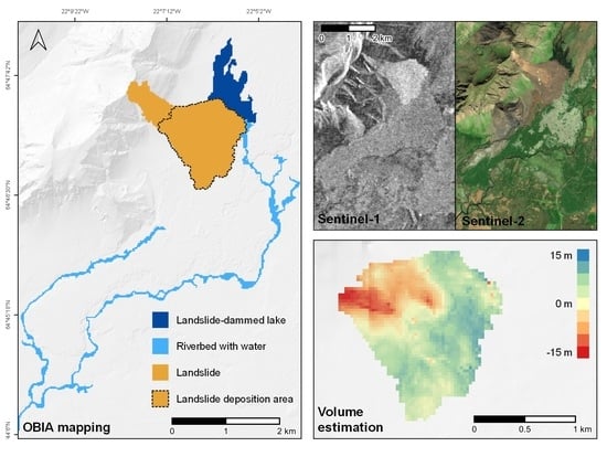
3.1. Geomorphological Features Mapping Using OBIA

The results of the geomorphological features mapping are shown in Figure 6. The pre-event result shows the original Hítará riverbed with water (Figure 6a). The post-event results (Figure 6b for 2018 and Figure 6c for 2019) show the landslide, the landslide-induced changes in the watercourse, and the landslide-dammed lake. The reference map from NLSI [77], which was used for comparison, is shown in Figure 6d. The water flowing out of the dammed lake found a new route through a lava field towards the south and then merged with the Stekka river, resulting in more water flowing in this riverbed than prior to the landslide. However, the upper part of the connection between the lake and the Stekka river is not easily distinguishable in the Sentinel-2 image taken in August 2019, probably due to less water flowing there at the time of the image acquisition one month later in the year 2019 (July 2018 versus August 2019). It seems that the Hítará river partly passes through the landslide and appears as a spring in the river bed downstream, i.e., approximately 2.5 km downstream from the lake and approximately 1 km downstream from the closest part of the landslide deposition. This is confirmed by the manually created reference data from NLSI [77]. The landslide area was estimated to be approximately 2000 ha in 2018 and 2019. Slight differences between the landslide areas likely result from variations in the segmentation. We estimated a lake area of 58 ha in 2018 and 47.1 ha in 2019. The reference values for the lake area are reported to be approximately 47 ha by Helgason et al. [45], but, the lake area from the shapefile provided by NLSI is 39.8 ha [77]. A comparison of our results with these numbers reveals an overestimation of the OBIA result for the year 2018. This could be associated with a high moisture content near the lakeshore and shallow water areas with high sediment load, which introduces uncertainty in the segmentation and classification [17]. The lower value for 2019 is probably due to the warm summer in 2019, which caused the discharge of some rivers to be lower for a few weeks [85].
The maximum width of the landslide deposition is approximately 1.5 km, and the overall runout length of the landslide is approximately 2.3 km. These results are in line with the numbers reported by Helgason et al. [45].

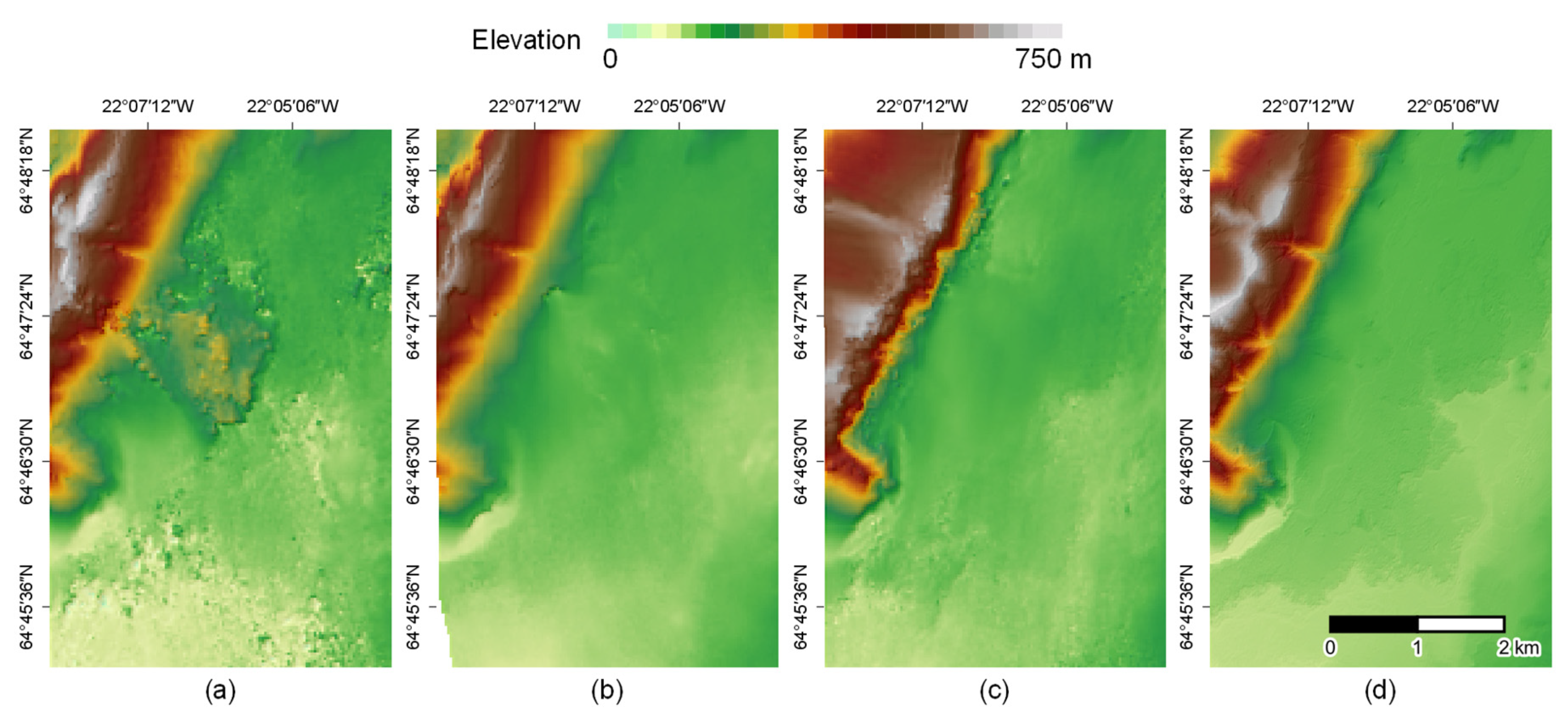
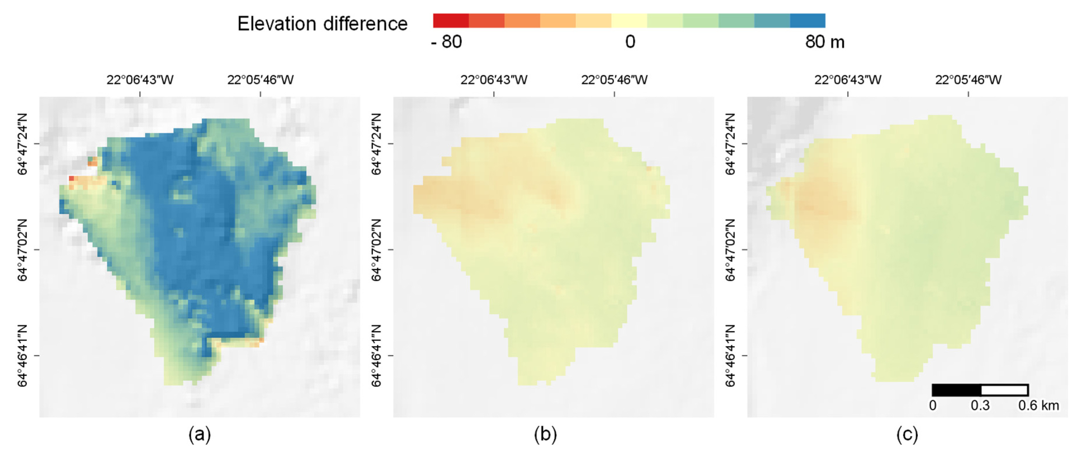
3.2. DEMs from Sentinel-1 and Landslide Volume Estimation

Figure 7 shows the results of the post-event DEMs generated using the Sentinel-1 image pairs from different orbit tracks, and the pre-event ArcticDEM for comparison.
For the volume estimation of the landslide, each of the three generated DEMs was subtracted from the ArcticDEM. Then a spatial subset for the landslide was created using the OBIA delineation of the landslide deposition area for 2018 (Figure 8). The DEM from track 16 shows maximum elevation differences to the ArcticDEM of more than 80 m, whereas the other two DEMs (track number 118 and 155) show lower, more homogenous and realistic elevation differences in the landslide deposition area. However, both DEMs from tracks 118 and 155 partly show negative values upslope, which indicate the removal of material and potential issues in the delineation of the deposition area.
Table 3 shows the landslide deposition volumes. The DEM from track 16 gives a much higher volume than the other two DEMs. The landslide volume estimations using the DEMs from track 118 and 155 are in a similar range.

3.3. DEM Validation

Table 4 shows the measures used for the accuracy assessment of the generated DEMs. The comparison of the statistical measures shows an underestimation of the minimum DEM value for the track 16 DEM, while the other two DEMs show similar minimum statistics as the ArcticDEM. In contrast, the maximum value for the track 16 DEM is the closest compared to the ArcticDEM while the other two DEMs (tracks 118 and 155) show lower values. The mean and standard deviation values for the track 16 DEM are closer to the values of the ArcticDEM.
The RMSE for the track 16 DEM is the lowest of the three DEMs, which indicates less vertical variation between track 16 and the ArcticDEM, but at the same time it has the lowest Moran’s I autocorrelation (0.92), which could be a result of the existence of more outliers compared to the track 118 and 155 DEMs, both of which have a Moran’s I of 0.97. The latter DEMs have better autocorrelation due to more homogenous values.
It is worth mentioning that both quality assessment indicators used (i.e., RMSE and Moran’s I) are global indicators, and they don’t take into account local variations.
From the statistics in Table 4, it is challenging to choose the most suitable DEM for volume estimation. Despite a clear indication of which DEM should give the best results, we see major differences in the measured volumes for the three DEMs (track 16, 118, and 155). According to the available literature [45], approximately 7 million m3 of material was released from the landslide source area, and the volume of the debris in the depositions area is about 10–20 million m3. According to these statistics, the track 16 DEM shows an unrealistic value of 109 million m3, whereas the landslide volumes calculated from the other two DEMs are closer to the estimated reference value.

4. Discussion

During the last two decades, OBIA has been used for many applications [28,29]. This research shows the advantage of integrating backscatter information from Sentinel-1 SAR data and spectral information from Sentinel-2 optical data within an expert knowledge-based classification approach in an OBIA environment to assess landslide-induced geomorphological changes. We used Hítardalur as a case study, where a large landslide blocked the river, and, consequently, a lake formed and the river changed its direction. The OBIA classification results show no significant change in the landslide area in the year after the event, but changes in the area of the landslide-dammed lake were detected. However, this might be partly explained by uncertainties in image segmentation and classification and seasonal variations due to different acquisition dates (July 2018 versus August 2019). Moreover, the spatial resolution of Sentinel-1 and Sentinel-2 images are limiting factors for river classification. Therefore, we first identified the existing riverbeds based on an edge detection layer and then assessed whether water was present in the riverbeds.
The Hítardalur landslide has several interesting characteristics that make it suitable to be considered as a case study for creating DEMs using Sentinel-1 datasets. It is a large landslide with a deposition area spreading over the rather flat valley. Therefore, both ascending and descending Sentinel-1 datasets can be used. The resolution and accuracy of DEMs have a direct influence on subsequent analyses such as the landform classification and hydrological modeling [86]. We applied a straightforward workflow for generating DEM using Sentinel-1 image pairs from three different tracks. Our results are heterogeneous and indicate that the generation of DEMs has several limitations in this situation. InSAR techniques have been extensively used for DEM generation using SAR datasets, but the accuracy of the resulting DEMs depends on several factors related to the data and processing workflows and techniques. For selecting suitable SAR datasets, the orbit indetermination and Bperp range, atmospheric conditions, and temporal decorrelation (due to scene changes between the two passes) need to be considered. To achieve a good vertical accuracy, the SAR image pair requires a large Bperp [76]. The Sentinel-1 mission was mainly designed for the retrieval of surface deformations using differential InSAR (DInSAR) which requires a low Bperp between consecutive SAR images, and DEM generation was not the primary goal of the mission [58]. The recommended Bperp for the DEM generation using the ERS satellite is between 150 and 300 m [57,87], but the ERS satellite is known to have high Bperp, whereas the common Bperp for Sentinel-1 datasets is below 30 m, which is very suitable for interferometry analysis but challenging for DEM generation [88,89]. In this study, we selected datasets in the Bperp range of 130 to 160 m, with a short temporal baseline of 6 days between each image pair. The temporal baseline is important to reduce phase noise. Although radar imagery is known for its all-weather measurement capability, changes in the atmospheric conditions (mainly water vapor) cause a variable path delay which results in atmospheric distortions and is the main error source in repeat-pass SAR interferometry [62]. In Iceland, the atmospheric and weather conditions make it difficult to find Sentinel-1 image pairs with a suitable Bperp and short temporal interval [90]. Therefore, we limited our search to the summer months (June to September), also to avoid snow cover. We also considered the coherency and the height ambiguity in our data selection. We selected three SAR image pairs from different orbit tracks, i.e., track 16 (11 July 2018 and 17 July 2018) and track 118 (5 August 2018 and 11 August 2018) for the ascending flight direction and track 155 (4 July 2019 and 10 July 2019) for the descending flight direction. One of the selected image pairs was in the range of the recommended Bperp, i.e., track number 155 with a Bperp of 159. This image pair also showed the lowest height ambiguity (98) compared to the others. The other two image pairs had a slightly lower Bperp (134 for track 16 and 142 for track 118) than recommended, but when considering the other selection criteria, they seemed to be the best datasets available.
We faced challenges in validating our classification and DEM-generated results. One issue was the availability of reference data. We used the values provided by Helgason et al. [45] as a reference for our classification and landslide volume estimation. Our volume estimations need to be considered with care since there are several uncertainties associated with them, and certain limitations make the comparison difficult. For example, the area used for the calculation of the landslide volume is not entirely clear and most likely differs from the delineation we used. We used the landslide deposition area, which was semi-automatically extracted using OBIA. Therefore, a one to one comparison of our results with other results reported in literature is not possible. Another challenge is directly related to the reliability of using the generated DEMs for volume calculations. We directly used the generated DEM from the InSAR processing workflow for volume estimation without any further post-processing, while the literature suggests that the InSAR-produced DEMs should be further post-processed to be ready for the end-user [42]. However, since we aimed to test the suitability of DEMs for landslide volume estimation created through a straightforward workflow that could be directly transferred to other areas, we did not apply any post-pressing to improve the volume estimation results. In this study, we demonstrated the potential and limitations inherent to the approach and the Sentinel-1 datasets for DEM generation. Thus, we did not apply any vertical correction on the DEMs generated from Sentinel-1 datasets. We did not use any pre-event DEM generated with this workflow. This was mainly to avoid introducing further errors to the volume estimation. However, there are several possibilities to deal with error distribution in the InSAR-generated DEMs, such as the fusion of the final products from the ascending and descending flight directions [32,91] and the horizontal and vertical adjustment of pixels in the post- and pre-event DEMs, to match them better and make the direct comparison more reliable [92]. Further work is needed to fully evaluate such approaches and the potential of using Sentinel-1 data to generate post-landslide event DEMs for volume estimation.

5. Conclusions

The combined use of Sentinel-1 and Sentinel-2 data offers opportunities for assessing landslides and landslide-induced geomorphological changes. Although many applications use EO datasets for landslide mapping [18,93], studies on integrating intensity information derived from Sentinel-1 SAR data with spectral information from Sentinel-2 optical data are still rare. In this study, we presented a semi-automated workflow to map the landslide-induced geomorphological changes in Hítardalur valley, Iceland, by jointly using Sentinel-1 and Sentinel-2 data within an OBIA framework and assessed the potential of post-event DEMs generated from Sentinel-1 image pairs from different orbit tracks for the estimation of the Hítardalur landslide volume.
It is plausible that we will face more frequent and large landslides in the future due to climate change. The high spatial and temporal resolution, free availability, and the integrated and effective use of Sentinel-1 and Sentinel-2 datasets can contribute enormously to analyzing such events and their consequences. However, the quality of post-event DEMs derived from Sentinel-1 data depends on several factors. These include the SAR image pair selection considering the perpendicular baseline, high coherency, and atmospheric conditions, as well as the process for DEM generation, for example, precise coregistration, phase unwrapping, and conversion of the unwrapped phase into elevation values. These are still active research areas [42]. Further research needs to be conducted to systematically assess the accuracy of the DEMs generated using Sentinel-1.

Author Contributions

Conceptualization: Z.D., D.H. and L.A.; Methodology: Z.D., D.H., L.A. and D.T.; Validation: Z.D., D.H., L.A. and J.K.H.; Formal Analysis: Z.D.; Investigation: Z.D., D.H., L.A., J.K.H. and Þ.S.; Data Creation, Z.D., D.H. and L.A.; Writing—Original Draft Preparation: Z.D. and D.H.; Writing—Review and Editing: Z.D., D.H., L.A., D.T., J.K.H. and Þ.S.; Visualization: Z.D., D.H., L.A.; Supervision: D.H.; Project Administration: D.H.; Funding Acquisition: D.H. and D.T. All authors have read and agreed to the published version of the manuscript.

Funding

This research has been supported by the Austrian Science Fund (FWF) through the project MORPH (Mapping, monitoring and modelling the spatio-temporal dynamics of land surface morphology; FWF-P29461-N29) and the Doctoral Collage GIScience (DK W 1237-N23), as well as by the Austrian Academy of Sciences (ÖAW) through the project RiCoLa (Detection and analysis of landslide-induced river course changes and lake formation).

Acknowledgments

The authors would like to thank S. Asgeirsson and M. Olafsson for providing field photographs.

Conflicts of Interest

The authors declare no conflict of interest.

Data Availability

Figure 6d shows the reference map from the National Land Survey of Iceland (NLSI) vector layer, available online at https://www.lmi.is (accessed on 15 May 2020); © NLSI (license: https://www.lmi.is/en/licence-for-national-land-survey-of-iceland-free-data (accessed on 15 May 2020)).

References

  1. Guzzetti, F.; Mondini, A.C.; Cardinali, M.; Fiorucci, F.; Santangelo, M.; Chang, K.-T. Landslide inventory maps: New tools for an old problem. Earth Sci. Rev. 2012, 112, 42–66. [Google Scholar] [CrossRef] [Green Version]
  2. Tacconi Stefanelli, C.; Casagli, N.; Catani, F. Landslide damming hazard susceptibility maps: A new GIS-based procedure for risk management. Landslides 2020, 17, 1635–1648. [Google Scholar] [CrossRef] [Green Version]
  3. Ermini, L.; Casagli, N. Prediction of the behaviour of landslide dams using a geomorphological dimensionless index. Earth Surf. Process Landf. 2003, 28, 31–47. [Google Scholar] [CrossRef]
  4. Sæmundsson, Þ.; Petursson, H.G.; Kneisel, C.; Beylich, A. Monitoring of the Tjarnardalir Landslide, in Central North Iceland. In Proceedings of the First North America Landslide Conference, Vail, CO, USA, 3–8 June 2007; Schaefer, V., Schuster, R., Turner, A., Eds.; AEG Publication: Madison, WI, USA, 2007; Volume 23, pp. 1029–1040. [Google Scholar]
  5. Decaulne, A. Slope processes and related risk appearance within the Icelandic Westfjords during the twentieth century. Nat. Hazards Earth Syst. Sci. 2005, 5, 309–318. [Google Scholar] [CrossRef] [Green Version]
  6. Sæmundsson, Þ.; Petursson, H. Causes and triggering factors for large scale displacements in the Almenningar landslide area, in central North Iceland. In Proceedings of the Geophysical Research Abstracts, Vienna, Austria, 8–13 April 2018; Volume 20. [Google Scholar]
  7. Sæmundsson, Þ.; Sigurðsson, I.; Pétursson, H.; Jónsson, H.; Decaulne, A.; Roberts, M.J.; Jensen, E.H. Bergflóðið sem féll á Morsárjökull 20. mars 2007—Hverjar hafa afleiðingar þess orðið? (The Morsárjökull rock avalanche in the southern part of the Vatnajökull glacier, south Iceland, in Icelandic). Náttúrufræðingurinn 2011, 81, 131–141. [Google Scholar]
  8. Sæmundsson, Þ.; Morino, C.; Helgason, J.K.; Conway, S.J.; Pétursson, H.G. The triggering factors of the Móafellshyrna debris slide in northern Iceland: Intense precipitation, earthquake activity and thawing of mountain permafrost. Sci. Total Environ. 2018, 621, 1163–1175. [Google Scholar] [CrossRef]
  9. Helgason, J.K.; Gylfadóttir, S.S.; Brynjólfsson, S.; Grímsdóttir, H.; Höskuldsson, Á.; Sæmundsson, Þ.; Hjartardóttir, Á.R.; Sigmundsson, F.; Jóhannesson, T. Berghlaupið í Öskju. 21. júlí 2014 (Rockslide in Askja on 21 July 2014, in Icelandic). Náttúrufræðingurinn 2019, 89, 5–21. [Google Scholar]
  10. Gylfadóttir, S.S.; Kim, J.; Helgason, J.K.; Brynjólfsson, S.; Höskuldsson, Á.; Jóhannesson, T.; Harbitz, C.B.; Løvholt, F. The 2014 Lake Askja rockslide-induced tsunami: Optimization of numerical tsunami model using observed data. J. Geophys. Res. Oceans 2017, 122, 4110–4122. [Google Scholar] [CrossRef] [Green Version]
  11. Jóhannesson, T.; Helgason, J.K.; Gylfadóttir, S.S. Comment on “Dynamics of the Askja caldera July 2014 landslide, Iceland, from seismic signal analysis: Precursor, motion and aftermath” by Schöpa et al. (2018). Earth Surf. Dyn. 2020, 8, 173–175. [Google Scholar] [CrossRef]
  12. Scaioni, M.; Longoni, L.; Melillo, V.; Papini, M. Remote Sensing for Landslide Investigations: An Overview of Recent Achievements and Perspectives. Remote Sens. 2014, 6, 9600–9652. [Google Scholar] [CrossRef] [Green Version]
  13. Joyce, K.E.; Belliss, S.E.; Samsonov, S.V.; McNeill, S.J.; Glassey, P.J. A review of the status of satellite remote sensing and image processing techniques for mapping natural hazards and disasters. Prog. Phys. Geogr. Earth Environ. 2009, 33, 183–207. [Google Scholar] [CrossRef] [Green Version]
  14. Casagli, N.; Cigna, F.; Bianchini, S.; Hölbling, D.; Füreder, P.; Righini, G.; Del Conte, S.; Friedl, B.; Schneiderbauer, S.; Iasio, C.; et al. Landslide mapping and monitoring by using radar and optical remote sensing: Examples from the EC-FP7 project SAFER. Remote Sens. Appl. Soc. Environ. 2016, 4, 92–108. [Google Scholar] [CrossRef] [Green Version]
  15. Hervás, J.; Barredo, J.I.; Rosin, P.L.; Pasuto, A.; Mantovani, F.; Silvano, S. Monitoring landslides from optical remotely sensed imagery: The case history of Tessina landslide, Italy. Geomorphology 2003, 54, 63–75. [Google Scholar] [CrossRef]
  16. Fiorucci, F.; Cardinali, M.; Carlà, R.; Rossi, M.; Mondini, A.C.; Santurri, L.; Ardizzone, F.; Guzzetti, F. Seasonal landslide mapping and estimation of landslide mobilization rates using aerial and satellite images. Geomorphology 2011, 129, 59–70. [Google Scholar] [CrossRef]
  17. Hölbling, D.; Abad, L.; Dabiri, Z.; Prasicek, G.; Tsai, T.; Argentin, A.-L. Mapping and Analyzing the Evolution of the Butangbunasi Landslide Using Landsat Time Series with Respect to Heavy Rainfall Events during Typhoons. Appl. Sci. 2020, 10, 630. [Google Scholar] [CrossRef] [Green Version]
  18. Zhong, C.; Liu, Y.; Gao, P.; Chen, W.; Li, H.; Hou, Y.; Nuremanguli, T.; Ma, H. Landslide mapping with remote sensing: Challenges and opportunities. Int. J. Remote Sens. 2020, 41, 1555–1581. [Google Scholar] [CrossRef]
  19. Lee, J.-S.; Pottier, E. Polarimetric Radar Imaging; CRC Press: Boca Raton, FL, USA, 2017; ISBN 9781315219332. [Google Scholar]
  20. Jensen, J.R. Introductory Digital Image Processing: A Remote Sensing Perspective, 4th ed.; Pearson Education, Incorporated: New York City, NY, USA, 2016; ISBN 978-0134058160. [Google Scholar]
  21. Jensen, J.R. Remote Sensing of the Environment: An Earth Resource Perspective, 2nd ed.; Prentice Hall series in Geographic Information Science; Pearson Prentice Hall: Upper Saddle River, NJ, USA, 2009; ISBN 9788131716809. [Google Scholar]
  22. Shirvani, Z. A Holistic Analysis for Landslide Susceptibility Mapping Applying Geographic Object-Based Random Forest: A Comparison between Protected and Non-Protected Forests. Remote Sens. 2020, 12, 434. [Google Scholar] [CrossRef] [Green Version]
  23. Plank, S.; Hölbling, D.; Eisank, C.; Friedl, B.; Martinis, S.; Twele, A. Comparing object-based landslide detection methods based on polarimetric SAR and optical satellite imagery—A case study in Taiwan. In Proceedings of the 7th International Workshop on Science and Applications of SAR Polarimetry and Polarimetric Interferometry, POLinSAR 2015, Frascati, Italy, 26–30 January 2015; pp. 1–5. [Google Scholar]
  24. Hölbling, D.; Friedl, B.; Dittrich, J.; Cigna, F.; Pedersen, G. Combined interpretation of optical and SAR data for landslide mapping. In Advances in Landslide Research, Proceedings of the 3rd Regional Symposium on Landslides the Adriatic-Balkan Region, Ljubljana, Slovenia, 11–13 October 2017; Jemec Auflic, M., Mikos, M., Verbovsek, T., Eds.; Geological Survey of Slovenia: Ljubljana, Slovenia, 2018; pp. 11–13. [Google Scholar]
  25. Plank, S.; Twele, A.; Martinis, S. Landslide Mapping in Vegetated Areas Using Change Detection Based on Optical and Polarimetric SAR Data. Remote Sens. 2016, 8, 307. [Google Scholar] [CrossRef] [Green Version]
  26. Moosavi, V.; Talebi, A.; Shirmohammadi, B. Producing a landslide inventory map using pixel-based and object-oriented approaches optimized by Taguchi method. Geomorphology 2014, 204, 646–656. [Google Scholar] [CrossRef]
  27. Keyport, R.N.; Oommen, T.; Martha, T.R.; Sajinkumar, K.S.; Gierke, J.S. A comparative analysis of pixel- and object-based detection of landslides from very high-resolution images. Int. J. Appl. Earth Obs. Geoinf. 2018, 64, 1–11. [Google Scholar] [CrossRef]
  28. Chen, G.; Weng, Q.; Hay, G.J.; He, Y. Geographic object-based image analysis (GEOBIA): Emerging trends and future opportunities. GISci. Remote Sens. 2018, 55, 159–182. [Google Scholar] [CrossRef]
  29. Blaschke, T.; Hay, G.J.; Kelly, M.; Lang, S.; Hofmann, P.; Addink, E.; Queiroz Feitosa, R.; van der Meer, F.; van der Werff, H.; van Coillie, F.; et al. Geographic Object-Based Image Analysis—Towards a new paradigm. ISPRS J. Photogramm. Remote Sens. 2014, 87, 180–191. [Google Scholar] [CrossRef] [PubMed] [Green Version]
  30. Hölbling, D.; Eisank, C.; Albrecht, F.; Vecchiotti, F.; Friedl, B.; Weinke, E.; Kociu, A. Comparing Manual and Semi-Automated Landslide Mapping Based on Optical Satellite Images from Different Sensors. Geosciences 2017, 7, 37. [Google Scholar] [CrossRef] [Green Version]
  31. Tsutsui, K.; Rokugawa, S.; Nakagawa, H.; Miyazaki, S.; Cheng, C.-T.; Shiraishi, T.; Yang, S.-D. Detection and Volume Estimation of Large-Scale Landslides Based on Elevation-Change Analysis Using DEMs Extracted From High-Resolution Satellite Stereo Imagery. IEEE Trans. Geosci. Remote Sens. 2007, 45, 1681–1696. [Google Scholar] [CrossRef]
  32. Crosetto, M. Calibration and validation of SAR interferometry for DEM generation. ISPRS J. Photogramm. Remote Sens. 2002, 57, 213–227. [Google Scholar] [CrossRef]
  33. Rosen, P.A.; Hensley, S.; Joughin, I.R.; Li, F.K.; Madsen, S.N.; Rodriguez, E.; Goldstein, R.M. Synthetic aperture radar interferometry. Proc. IEEE 2000, 88, 333–382. [Google Scholar] [CrossRef]
  34. Gens, R.; van Genderen, J.L. Review Article SAR interferometry—Issues, techniques, applications. Int. J. Remote Sens. 1996, 17, 1803–1835. [Google Scholar] [CrossRef]
  35. Haghighi, M.H.; Motagh, M. Sentinel-1 InSAR over Germany: Large-scale interferometry, atmospheric effects, and ground deformation mapping. ZFV—Z. Geodasie Geoinf. Landmanag. 2017, 142, 245–256. [Google Scholar]
  36. Yang, L.; Meng, X.; Zhang, X. SRTM DEM and its application advances. Int. J. Remote Sens. 2011, 32, 3875–3896. [Google Scholar] [CrossRef]
  37. Drusch, M.; Del Bello, U.; Carlier, S.; Colin, O.; Fernandez, V.; Gascon, F.; Hoersch, B.; Isola, C.; Laberinti, P.; Martimort, P.; et al. Sentinel-2: ESA’s Optical High-Resolution Mission for GMES Operational Services. Remote Sens. Environ. 2012, 120, 25–36. [Google Scholar] [CrossRef]
  38. Torres, R.; Snoeij, P.; Geudtner, D.; Bibby, D.; Davidson, M.; Attema, E.; Potin, P.; Rommen, B.; Floury, N.; Brown, M.; et al. GMES Sentinel-1 mission. Remote Sens. Environ. 2012, 120, 9–24. [Google Scholar] [CrossRef]
  39. Ottavianello, G. Copernicus Space Component Data Access Portfolio: Data Warehouse 2014–2020; European Space Agency: Frascati, Italy, 2019. [Google Scholar]
  40. De Zan, F.; Monti Guarnieri, A. TOPSAR: Terrain Observation by Progressive Scans. IEEE Trans. Geosci. Remote Sens. 2006, 44, 2352–2360. [Google Scholar] [CrossRef]
  41. Farkas, P.; Hevér, R.; Grenerczy, G. Geodetic integration of Sentinel-1A IW data using PSInSAR in Hungary. In Proceedings of the Geophysical Research Abstracts, Vienna, Austria, 12–17 April 2015; Volume 17. [Google Scholar]
  42. Dai, K.; Li, Z.; Tomás, R.; Liu, G.; Yu, B.; Wang, X.; Cheng, H.; Chen, J.; Stockamp, J. Monitoring activity at the Daguangbao mega-landslide (China) using Sentinel-1 TOPS time series interferometry. Remote Sens. Environ. 2016, 186, 501–513. [Google Scholar] [CrossRef] [Green Version]
  43. Kyriou, A.; Nikolakopoulos, K. Landslide mapping using optical and radar data: A case study from Aminteo, Western Macedonia Greece. Eur. J. Remote Sens. 2019, 1–11. [Google Scholar] [CrossRef] [Green Version]
  44. Barra, A.; Monserrat, O.; Mazzanti, P.; Esposito, C.; Crosetto, M.; Scarascia Mugnozza, G. First insights on the potential of Sentinel-1 for landslides detection. Geomat. Nat. Hazards Risk 2016, 7, 1874–1883. [Google Scholar] [CrossRef] [Green Version]
  45. Helgason, J.K.; Sæmundsson, Þ.; Drouin, V.; Jóhannesson, T. The Hítardalur landslide in West Iceland in July 2018. In Proceedings of the Geophysical Research Abstracts, Vienna, Austria, 7–12 April 2019; Volume 21. [Google Scholar]
  46. Jordan, B.T.; Carley, T.L.; Banik, T.J. Iceland: The Formation and Evolution of a Young, Dynamic, Volcanic Island—A Field Trip Guide. In Iceland: The Formation and Evolution of a Young, Dynamic, Volcanic Island—A Field Trip Guide; Geological Society of America: Boulder, CO, USA, 2019; Volume 54, ISBN 9780813700540. [Google Scholar]
  47. Ragnarsdóttir, K.V. Jarðlagaskipan Fagraskógarfjalls og Vatnshlíðar í Hítardal (Geology of Mt. Fagraskógarfjall and Mt. Vatnshlíðarfjall in Hítardalur Valley, in Icelandic); University of Iceland: Reykjavík, Iceland, 1979. [Google Scholar]
  48. Johannesson, H. Jarlagaskipan og róun rekbelta á Vesturlandi (Stratigraphy and development of spreading centers in Western Iceland, in Icelandic). Náttórufrœingurinn 1980, 50, 13–31. [Google Scholar]
  49. Larkin, H.; Magnall, N.; Thomas, A.; Holley, R.; Mccormack, H. Utilising satellite-based techniques to identify and monitor slope instabilities: The Fagraskógarfjall and Limnes landslides. In Proceedings of the 2020 International Symposium on Slope Stability in Open Pit Mining and Civil Engineering, Australian Centre for Geomechanics, Perth, Australia, 12–14 May 2020; pp. 1455–1466. [Google Scholar]
  50. Iceland Met Office (IMO). A Large Landslide Falls in Hítardalur Valley. Available online: https://en.vedur.is/about-imo/news/a-large-landslide-falls-in-hitardalur-valley (accessed on 11 August 2020).
  51. Pétursson, H.G. Large Landslides Since the Middle of the Last Century. Available online: https://en.vedur.is/media/frettir-myndasafn-2018/Big_landslides_Table_ENG.pdf (accessed on 17 June 2020).
  52. Wegnüller, U.; Werner, C.; Strozzi, T.; Wiesmann, A.; Frey, O.; Santoro, M. Sentinel-1 Support in the GAMMA Software. Procedia Comput. Sci. 2016, 100, 1305–1312. [Google Scholar] [CrossRef] [Green Version]
  53. Lee, J.-S. Refined filtering of image noise using local statistics. Comput. Graph. Image Process. 1981, 15, 380–389. [Google Scholar] [CrossRef]
  54. Yommy, A.S.; Liu, R.; Wu, A.S. SAR Image Despeckling Using Refined Lee Filter. In Proceedings of the 2015 7th International Conference on Intelligent Human-Machine Systems and Cybernetics, Hangzhou, China, 26–27 August 2015; Volume 2, pp. 260–265. [Google Scholar]
  55. Park, J.-W.; Korosov, A.A.; Babiker, M.; Sandven, S.; Won, J.-S. Efficient Thermal Noise Removal for Sentinel-1 TOPSAR Cross-Polarization Channel. IEEE Trans. Geosci. Remote Sens. 2018, 56, 1555–1565. [Google Scholar] [CrossRef]
  56. Filipponi, F. Sentinel-1 GRD Preprocessing Workflow. Proceedings 2019, 18, 11. [Google Scholar] [CrossRef] [Green Version]
  57. Ferretti, A.; Monti Guarnieri, A.; Prati, C.; Rocca, F. InSAR Principles: Guidelines for SAR Interferometry Processing and Interpretation; Fletcher, K., Ed.; ESA Publications: Noordwijk, The Netherlands, 2007; ISBN 92-9092-233-8. [Google Scholar]
  58. Geudtner, D.; Prats, P.; Yague-Martinez, N.; Navas-Traver, I.; Barat, I.; Torres, R.R. Sentinel-1 SAR interferometry performance verification. In Proceedings of the 11th European Conference on Synthetic Aperture Radar, EUSAR, Berlin, Germany, 6–9 June 2016; VDE VERLAG GMBH: Berlin, Germany, 2016; pp. 65–68. [Google Scholar]
  59. Kyriou, A.; Nikolakopoulos, K. Assessing the suitability of Sentinel-1 data for landslide mapping. Eur. J. Remote Sens. 2018, 51, 402–411. [Google Scholar] [CrossRef] [Green Version]
  60. Bürgmann, R.; Rosen, P.A.; Fielding, E.J. Synthetic Aperture Radar Interferometry to Measure Earth’s Surface Topography and Its Deformation. Annu. Rev. Earth Planet. Sci. 2000, 28, 169–209. [Google Scholar] [CrossRef]
  61. Rott, H.; Nagler, T. The contribution of radar interferometry to the assessment of landslide hazards. Adv. Space Res. 2006, 37, 710–719. [Google Scholar] [CrossRef]
  62. Wegmüller, U.; Santoro, M.; Werner, C.; Strozzi, T.; Wiesmann, A.; Lengert, W. DEM generation using ERS–ENVISAT interferometry. J. Appl. Geophys. 2009, 69, 51–58. [Google Scholar] [CrossRef]
  63. Porter, C.; Morin, P.; Howat, I.; Noh, M.-J.; Bates, B.; Peterman, K.; Keesey, S.; Schlenk, M.; Gardiner, J.; Tomko, K.; et al. ArcticDEM. Harvard Dataverse; Polar Geospatial Center, University of Minnesota: Minneapolis, MN, USA, 2018; Volume 1. [Google Scholar]
  64. Schumann, G.J.-P.; Bates, P.D. The Need for a High-Accuracy, Open-Access Global DEM. Front. Earth Sci. 2018, 6, 225. [Google Scholar] [CrossRef]
  65. Lee, J.-S. NOTE Digital Image Smoothing and the Sigma Filter. Comput. Vision Graph. Image Process. 1983, 24, 255–269. [Google Scholar] [CrossRef]
  66. Baatz, M.; Schäpe, A. Multiresolution Segmentation: An optimization approach for high quality multi-scale image segmentation. In Proceedings of the Angewandte Geographische Informationsverarbeitung XII; Strobl, J., Blaschke, T., Griesebner, G., Eds.; Wichmann: Heidelberg, Germany, 2000; pp. 12–23. [Google Scholar]
  67. Eisank, C.; Smith, M.; Hillier, J. Assessment of multiresolution segmentation for delimiting drumlins in digital elevation models. Geomorphology 2014, 214, 452–464. [Google Scholar] [CrossRef] [Green Version]
  68. Yague-Martinez, N.; Prats-Iraola, P.; Rodriguez Gonzalez, F.; Brcic, R.; Shau, R.; Geudtner, D.; Eineder, M.; Bamler, R. Interferometric Processing of Sentinel-1 TOPS Data. IEEE Trans. Geosci. Remote Sens. 2016, 54, 2220–2234. [Google Scholar] [CrossRef] [Green Version]
  69. Lazecký, M.; Hlaváčová, I.; Martinovič, J.; Ruiz-Armenteros, A.M. Accuracy of Sentinel-1 Interferometry Monitoring System based on Topography-free Phase Images. Procedia Comput. Sci. 2018, 138, 310–317. [Google Scholar] [CrossRef]
  70. Goldstein, R.M.; Werner, C.L. Radar interferogram filtering for geophysical applications. Geophys. Res. Lett. 1998, 25, 4035–4038. [Google Scholar] [CrossRef] [Green Version]
  71. Lee, J.-S.; Hoppel, K.W.; Mango, S.A.; Miller, A.R. Intensity and phase statistics of multilook polarimetric and interferometric SAR imagery. IEEE Trans. Geosci. Remote Sens. 1994, 32, 1017–1028. [Google Scholar]
  72. Schmitt, A. Multiscale and Multidirectional Multilooking for SAR Image Enhancement. IEEE Trans. Geosci. Remote Sens. 2016, 54, 5117–5134. [Google Scholar] [CrossRef]
  73. Chen, C.W.; Zebker, H.A. Network approaches to two-dimensional phase unwrapping: Intractability and two new algorithms. J. Opt. Soc. Am. A 2000, 17, 401. [Google Scholar] [CrossRef]
  74. Chen, C.W.; Zebker, H.A. Phase unwrapping for large SAR interferograms: Statistical segmentation and generalized network models. IEEE Trans. Geosci. Remote Sens. 2002, 40, 1709–1719. [Google Scholar] [CrossRef] [Green Version]
  75. Chen, C.W.; Zebker, H.A. Two-dimensional phase unwrapping with use of statistical models for cost functions in nonlinear optimization. J. Opt. Soc. Am. A 2001, 18, 338. [Google Scholar] [CrossRef] [Green Version]
  76. Richards, M.A. A Beginner’s Guide to Interferometric SAR Concepts and Signal Processing [AESS Tutorial IV]. IEEE Aerosp. Electron. Syst. Mag. 2007, 22, 5–29. [Google Scholar] [CrossRef]
  77. National Land Survey of Iceland IS 50V 24/12 2019 Vatnafar Flakar. Available online: https://gatt.lmi.is/geonetwork/srv/eng/catalog.search#/metadata/83E61CBF-8498-4259-A40C-3B628EA34FB7 (accessed on 15 May 2020).
  78. Maune, D.F. Digital Elevation Model Technologies and Applications: The DEM Users Manual, 2nd ed.; American Society for Photogrammetry and Remote Sensing: Bethesda, MD, USA, 2007; ISBN 9781570830822. [Google Scholar]
  79. Höhle, J.; Höhle, M. Accuracy assessment of digital elevation models by means of robust statistical methods. ISPRS J. Photogramm. Remote Sens. 2009, 64, 398–406. [Google Scholar] [CrossRef] [Green Version]
  80. Candela, S.G.; Howat, I.; Noh, M.-J.; Porter, C.C.; Morin, P.J. ArcticDEM Validation and Accuracy Assessment. In Proceedings of the American Geophysical Union, Fall Meeting, New Orleans, LA, USA, 11–15 December 2017. [Google Scholar]
  81. Griffith, D. Spatial Autocorrelation: A Primer; Association of American Geographers: Washington, DC, USA, 1987; ISBN 9780892911974. [Google Scholar]
  82. Moran, P.A.P. The Interpretation of Statistical Maps. J. R. Stat. Soc. Ser. B 1948, 10, 243–251. [Google Scholar] [CrossRef]
  83. Wechsler, S.P. Perceptions of digital elevation model uncertainty by DEM users. URISA J. 2003, 15, 57–64. [Google Scholar]
  84. Wechsler, S.P.; Kroll, C.N. Quantifying DEM Uncertainty and its Effect on Topographic Parameters. Photogramm. Eng. Remote Sens. 2006, 72, 1081–1090. [Google Scholar] [CrossRef] [Green Version]
  85. Iceland Met Office (IMO). The Weather in Iceland in 2019. Available online: https://en.vedur.is/about-imo/news/the-weather-in-iceland-in-2019 (accessed on 15 May 2020).
  86. Kramm, T.; Hoffmeister, D. Evaluation of Digital Elevation Models for Geomorphometric Analyses on Different Scales for Northern Chile. ISPRS Int. Arch. Photogramm. Remote Sens. Spat. Inf. Sci. 2019, XLII-2/W13, 1229–1235. [Google Scholar] [CrossRef] [Green Version]
  87. Braun, A. DEM Generation with Sentinel-1 Workflow and Challenges; European Space Agency: Paris, France, 2020. [Google Scholar]
  88. Berardino, P.; Fornaro, G.; Lanari, R.; Sansosti, E. A new algorithm for surface deformation monitoring based on small baseline differential SAR interferograms. IEEE Trans. Geosci. Remote Sens. 2002, 40, 2375–2383. [Google Scholar] [CrossRef] [Green Version]
  89. Geudtner, D.; Torres, R.; Snoeij, P.; Davidson, M.; Rommen, B. Sentinel-1 System capabilities and applications. In Proceedings of the 2014 IEEE Geoscience and Remote Sensing Symposium, Quebec City, QC, Canada, 13–18 July 2014; pp. 1457–1460. [Google Scholar]
  90. Amitrano, D.; Guida, R.; Dell’Aglio, D.; Di Martino, G.; Di Martire, D.; Iodice, A.; Costantini, M.; Malvarosa, F.; Minati, F. Long-Term Satellite Monitoring of the Slumgullion Landslide Using Space-Borne Synthetic Aperture Radar Sub-Pixel Offset Tracking. Remote Sens. 2019, 11, 369. [Google Scholar] [CrossRef] [Green Version]
  91. Sansosti, E.; Lanari, R.; Fornaro, G.; Franceschetti, G.; Tesauro, M.; Puglisi, G.; Coltelli, M. Digital elevation model generation using ascending and descending ERS-1/ERS-2 tandem data. Int. J. Remote Sens. 1999, 20, 1527–1547. [Google Scholar] [CrossRef]
  92. Tang, C.; Tanyas, H.; van Westen, C.J.; Tang, C.; Fan, X.; Jetten, V.G. Analysing post-earthquake mass movement volume dynamics with multi-source DEMs. Eng. Geol. 2019, 248, 89–101. [Google Scholar] [CrossRef]
  93. Zhao, C.; Lu, Z. Remote Sensing of Landslides—A Review. Remote Sens. 2018, 10, 279. [Google Scholar] [CrossRef] [Green Version]
Figure 1. (a) The study area around the Hítardalur landslide shown on a Sentinel-2 image acquired on 17 July 2018 and (b) its location in western Iceland; background data © ESRI.
Applsci 10 05848 g001
Figure 2. (a) Photograph showing the Hítardalur landslide and the landslide-dammed lake soon after the event occurred, i.e., taken on the afternoon of 7 July 2018 (photograph: © S. Asgeirsson). (b) View from the landslide deposition area towards the landslide source area (photograph: © J. K. Helgason; 7 July 2018). (c) Water from the dammed lake finds a new way (photograph: © J. K. Helgason; 7 July 2018). (d) View from the Fagraskógarfjall mountain towards the Hítardalur valley showing the landslide deposition area and the new watercourse flowing out from the lake into the Stekka river (photograph: © M. Olafsson; 23 November 2018).
Applsci 10 05848 g002
Figure 3. Sentinel-1 and Sentinel-2 datasets used for geomorphological features mapping. The upper row shows the intensity layer for Sentinel-1 vertical-vertical (VV) polarization for the following image acquisition dates: (a) 5 July 2018; (b) 17 July 2018; (c) 5 August 2019. The lower row shows the true color composites of the Sentinel-2 images with the following acquisition dates: (d) 20 June 2018; (e) 17 July 2018; (f) 1 August 2019.
Applsci 10 05848 g003
Figure 4. Examples of the layers extracted from the Sentinel-1 and Sentinel-2 datasets. (a) and (b) show the subtraction layers using pre- and post-event Sentinel-1 VV polarization intensity images for 2018 and 2019, respectively. The Hítardalur landslide and the landslide-dammed lake are distinguishable. (c) and (d) show the edge extraction layers derived from the post-event Sentinel-2 images (Near-infrared (NIR) band (B8)) for 2018 and 2019, respectively.
Applsci 10 05848 g004
Figure 5. The classification framework used for the post-event geomorphological feature mapping for 2018 and 2019.
Applsci 10 05848 g005
Figure 6. Object-based geomorphological feature mapping using Sentinel-1 and Sentinel-2 datasets. (a) shows the riverbed with water before the Hítardalur landslide using the pre-event Sentinel-2 image only; (b) shows the landslide, the landslide deposition area, the landslide-dammed lake, and the (now partly interrupted) riverbeds with water after the landslide event in 2018; (c) shows the landslide, the landslide-dammed lake, and the riverbeds with water in 2019; (d) shows the reference map from National Land Survey of Iceland IS 50V 24 September 2019 Vatnafar Flakar (© NLSI) [77]. The hillshade derived from the ArcticDEM was used as a background layer.
Applsci 10 05848 g006
Figure 7. Illustration of the three post-event DEMs derived from the Sentinel-1 image pairs. (a) for orbit track number 16 (11 July 2018 and 17 July 2018), ascending; (b) orbit track number 118 (5 August 2018 and 11 August 2018), ascending; (c) orbit track number 155 (4 July 2019 and 10 July 219), descending; (d) ArcticDEM. For visualization purposes, each DEM is overlaid with the hillshade derived from it.
Applsci 10 05848 g007
Figure 8. Elevation differences of the three Sentinel-1 DEMs compared to the ArcticDEM for the landslide deposition area used for calculation of the landslide volume. (a) elevation differences of DEM from track 16 (11 July 2018 and 17 July 2018); (b) elevation differences of DEM from track 118 (5 August 2018 and 11 August 2018); (c) elevation differences of DEM from track 155 (4 July 2019 and 10 July 2019). The respective hillshade derived from the Sentinel-1 DEMs was overlaid for each result.
Applsci 10 05848 g008
Table 1. Sentinel-2 datasets used in this research. MSI stands for Multispectral Instrument.
DateSensor, ProductPre-/Post-Event
20 June 2018Sentinel-2 B MSI, Level-1CPre
17 July 2018Sentinel-2 B MSI, Level-1CPost
1 August 2019Sentinel-2 B MSI, Level-1CPost
Table 2. Sentinel-1 data and their characteristics used to generate the digital elevation models (DEMs). The Bperp stands for the spatial perpendicular baseline, which was used as the main criterion for the selection of Sentinel-1 A and B image pairs. The modeled coherency and height ambiguity measurements were derived using the interferometric synthetic aperture radar (SAR) (InSAR) stack overview function implemented in the Sentinel Application Platform (SNAP) toolbox.
Sentinel-1 Image PairsOrbit TrackFlight DirectionTime Baseline (Days)Bperp (m)Modeled CoherencyHeight Ambiguity (m)
11 July 2018 and
17 July 2018
16Ascending61340.88115
5 August 2018 and
11 August 2018
118Ascending61420.87110
4 July 2019 and
10 July 2019
155Descending61590.8698
Table 3. Volume estimation of the landslide based on the Sentinel-1 derived post-event DEMs and the pre-event ArcticDEM.
Sentinel-1 DEM Orbit TrackVolume (Million m3)
11 July 2018 and 17 July 2018 16109
5 August 2018 and 11 August 20181187
4 July 2019 and 10 July 201915512
Table 4. Validation of the Sentinel-1 DEMs with respect to the ArcticDEM. Comparison is based on the area not influenced by the landslide. The Moran’s I statistic is calculated on the difference map.
Acquisition DateOrbit TracksMin Elevation (m)Max
Elevation (m)
Mean Elevation (m)Std. Dev. (m)RMSE (m)Moran’s I
Arctic DEM
- 89743180117--
Post-event DEMs
11 July 2018
and
17 July 2018
1618750176115300.92
5 August 2018
11 August 2018
11878654173100370.97
4 July 2019
and
10 July 2019
15587681192130460.97

