RETRACTED: Reconstructing the Dynamic Processes of the Taimali Landslide in Taiwan Using the Waveform Inversion Method

Abstract

As a landslide occurs, seismic signals generated by the mass sliding on the slope can be recorded by seismometers nearby. Using waveform inversion techniques, we can explore the dynamic processes (e.g., sliding direction, velocity, and runout distance) of a landslide with the inverted force–time function. In this study, the point force history (PFH) inversion method was applied to the Taimali landslide in Taiwan, which was triggered by a heavy rainstorm in 2009. The inverted force–time function for the landslide revealed the complicated dynamic processes. The time series of velocity indicated three different sliding directions during the landslide. Hence, three propagating stages of the Taimali landslide were determined and were consistent with an investigation using remote sensing images and a digital elevation model of the landslide. In addition, the PFH inversion was implemented using high-quality single-station records and maintained good performance compared with the inversion by multistation records.

1. Introduction

Landslides caused by either earthquakes or rainfall have caused the destruction of public facilities, economic loss, and loss of life and property in Taiwan over the past few decades [1,2]. One of the severest slope disasters in Taiwan took place during Typhoon Morakot, which affected Taiwan from 8–10 August 2009. That disaster left nearly 700 persons dead or missing and caused about 3.3 billion USD in economic loss [2,3]. The unexpected heavy rainfall caused thousands of landslides and debris flows in southern Taiwan, including the giant Hsiaolin landslide and the Taimali landslide [2]. In particular, significantly more landslides with larger disturbed areas occurred during Typhoon Morakot in 2009 than during previous typhoon events. These giant landslides, known as large-scale landslides (LSLs), are defined as the landslides with areas of larger than 10⁵ m², volumes of more than 10⁶ m³, or depths greater than 10 m [4]. After Typhoon Morakot, the study of LSLs became one of the most important issues related to slope disasters in Taiwan. The features of LSLs include spontaneity, fast movement, and destruction; hence, landslide processes are a hard-to-observe natural phenomenon [5], and it is difficult to mitigate landslide disasters with traditional study methods.

A few studies have reported that block sliding processes on the slope would generate ground motions that can be recorded by seismic stations [5,6,7,8]. The landslide-generated ground motions contain low-frequency (<1 Hz) and high-frequency (>1 Hz) waves. The high-frequency waves are produced by the unloading and reloading cycle of the sliding materials [7], and the high-frequency waves result from the complex impacts between the sliding debris [8]. In the frequency domain, the landslide-induced seismic ground motions are mainly distributed below 10 Hz, and the energy signature in the spectrogram shows a triangular pattern from accumulation to dissipation due to the high-frequency constituents over time. The triangular signature in the spectrogram is a distinctive property enabling the differentiation of the landslide-induced signals from those generated by earthquakes and other ambient noise. If such ground motion is recorded by seismic stations, the timing of large landslides can be extracted, and the seismic interpretation can be used as precious information to calibrate numerical simulations [9]. Furthermore, waveform inversion techniques allow us to reconstruct sliding processes (e.g., sliding velocity, direction, and runout distance), so they are appropriate methods for research on the dynamic processes of landslides. After nearly a decade of development, different waveform inversion approaches have been proposed, and each has distinguishing features and advantages. Reviewing the achievements of different kinds of waveform inversion methods for large-scale landslides is vital for further application. In this study, a waveform inversion method was applied to the large-scale Taimali landslide.

2. Review of Waveform Inversion Methods for Reconstructing the Dynamic Processes of a Landslide

Waveform inversion methods for reconstructing the dynamic processes of a landslide can be traced back to Kanamori and Given [10,11]. So far, three waveform inversion methods have been widely used to study the dynamic processes of a landslide. The first one is a frequency-domain inversion method (FIM) proposed by Nakano et al. [12]. Lin et al. [13] used FIM with the seismic records of eight broadband seismic stations in Taiwan for the Hsiaolin landslide and obtained a maximum force of about 5 × 10¹⁰ N. Yamada et al. [14] also used FIM with seismic records of six stations for the Akatani landslide in Japan. The variations of frictional coefficients of the Akatani landslide were calculated, and their range was 0.38–0.56.

The second one is the landslide force history (LFH) inversion method proposed by Ekstrom et al. [7]. LFH is based on the assumption that the block mass becomes decoupled from the sliding surface and induces forces on the slope during the movement of the landslide mass. Seismic waves are generated by this time-varying force acting on the sliding surface. The three-component (east, north, and vertical) force is parameterized as a sequence of partially overlapping isosceles triangles to synthesize a landslide force history. Hibert et al. [5], Hibert et al. [15], and Chao et al. [16] applied LFH to the Bingham Canyon Mine in the USA, the Oso landslide in the USA, and several landslides in Taiwan, respectively. The LFH method is executed in the time domain. The relationships between the maximum force and surface wave magnitude, landslide mass, and maximum momentum have been investigated through the inversion results by using the LFH method.

The third method is the point force history (PFH) inversion method proposed by Allstadt [17], which is executed in the time domain and based on the assumption that a landslide can be simplified as a stationary, constant mass block sliding on a slope. Allstadt [17] applied the PFH method to the Mount Meager rockslide–debris flow in British Columbia and figured out that the frictional coefficient of the rockslide–debris flow was about 0.38 ± 0.02. Iverson et al. [18] also used the PFH method for the Oso landslide in the USA and compared the inversion results with the numerical modeling results.

In summary, despite the operating environments (e.g., time and frequency domains), the three common inversion methods can provide information on the dynamic processes of landslide movement, such as force magnitude, sliding velocity, frictional coefficient, and runout distance. Based on the literature studies, it is found that the PFH can be an efficient and practical method as it is less time-consuming and can be performed with fewer data recorded from seismic stations. In this study, the PFH method was applied to a large-scale landslide, the Taimali landslide. The inversion results were used to reconstruct the dynamic processes of the giant landslide.

3. Study Case and Method

3.1. Taimali Landslide

On 9 August 2009, at 17:31 local time (UTC + 8), a large-scale landslide took place in the upstream area of the Taimali River in southeastern Taiwan (120.81° E, 22.55° N) (Figure 1). The main trigger of the landslide was a violent rainstorm brought by Typhoon Morakot, which induced cumulative rainfall exceeding 2000 mm in three days [19]. Despite the numerous landslides of the preceding decades, the Taimali landslide was one of the largest landslides ever recorded in Taiwan. It generated clear and adequate seismic signals for the seismic and waveform inversion analyses.

The Taimali landslide is located on the Eocene Bilusan Formation composed of phyllite and slate with sandstone interbeds [20]. Folds and cleavages are also well developed in this region and hence lead to the fractured geologic condition of the Taimali landslide. According to the Central Geological Survey [21], a region-scale anticlinorium lies to the west of the Taimali landslide and is seven kilometers from the landslide. The source area of the Taimali landslide was on a dip slope and prone to collapse during heavy rainfall.

Pre- and post-event digital elevation models (DEMs) with resolutions of five meters were used to map the disturbed area of the landslide and to calculate the variance in topography (Figure 2). The main source area (Zone 1) was about 9.3 × 10⁵ m², and its total volume was about 7.5 × 10⁷ m³. The maximum depth, roughly at the center of the landslide block, was 220 m. Based on the variance in topography, two deposit areas (Zone 2 and 3) could be recognized. The thickness of the landslide deposit in Zone 2 was thicker than that in Zone 3 (

Table 1. Measurements of the source area and the deposit areas.

Zone	Area (106 m2)	Maximum Thickness (m)	Average Thickness (m)	Volume (106 m3)	Estimated Mass (106 kg)
1	0.93	219.7	80.9	75	20
2	1.24	196.9	96.9	45	12
3	1.22	110.6	67.2	43	12

). This difference indicated that Zone 2 might be the main deposit area for this event. A relatively smaller landslide (3 × 10⁵ m²) occurred and provided some amount of debris to the deposit area (Zone 2 and Zone 3). Because the volume of the smaller source was not considered, the sum of the volume of the two major deposit areas is greater than the volume of the only major source area. Based on the average density of 2700 kg/m³ for phyllite, the mass of the Taimali landslide was estimated at 2 × 10¹¹ kg, and therefore it generated high-energy seismic signals.

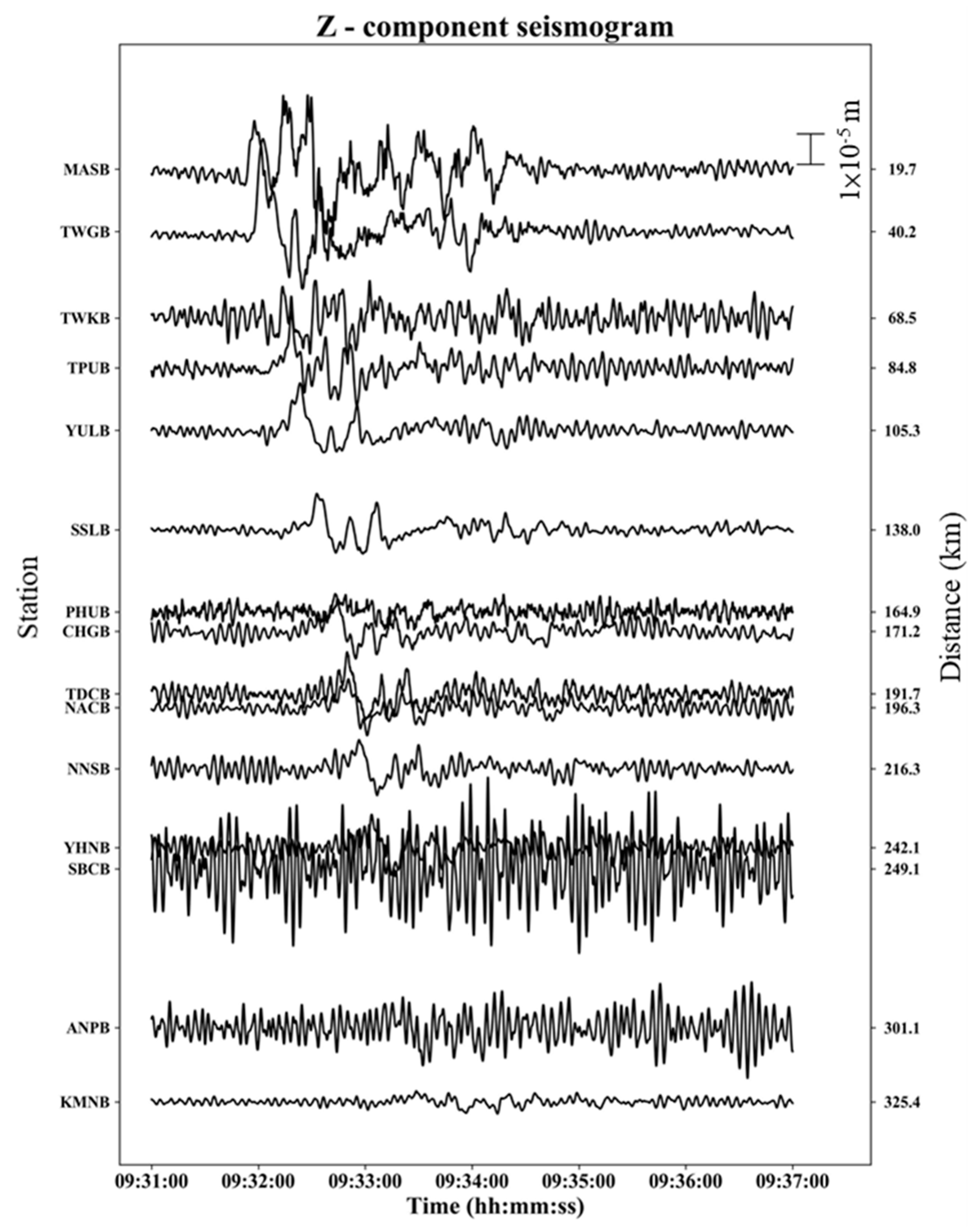
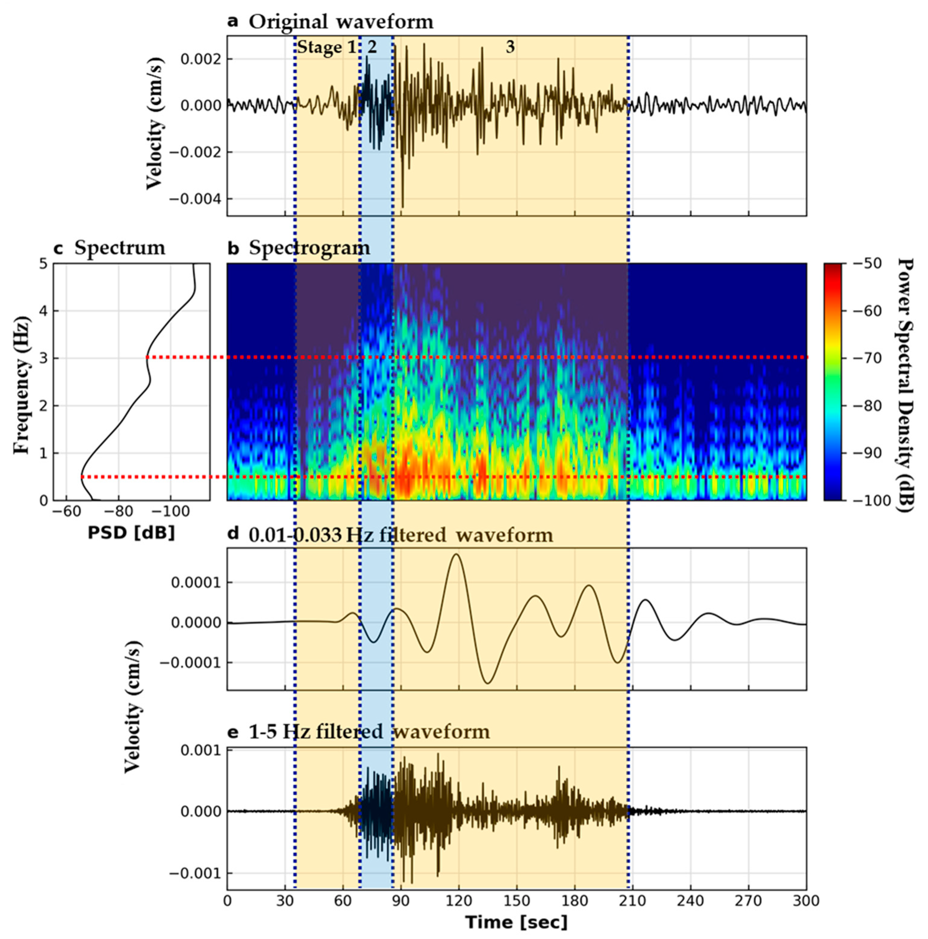
3.2. Seismic Data Processing

In this study, the seismic data recorded by broadband seismic stations were collected from the Broadband Array in Taiwan for Seismology (BATS), which was deployed by Academia Sinica and Taiwan’s Central Weather Bureau (CWB) since 1992 [22]. BATS provides high-precision continuous seismic records to document the ground motions of landslides. All permanent BATS stations are equipped with broadband sensors with a frequency band of 0.00833–8 Hz. All stations are capable of internet connection for immediate retrieval of real-time data. The high-energy seismic signals generated by the Taimali landslide were detected by 15 three-component broadband seismometers (Figure 3), including the nearest station, MASB, at a distance of 19 km, and the farthest station, KMNB, at a distance of 325 km. Even in the Taiwan Strait, the seismic signals caused by the landslide could be detected by the PHUB and KMNB stations on small islands.

The ground motion induced by the Taimali landslide can be observed in the seismic record at the MASB station (Figure 4a). However, it is not easy to determine the initiation time and end time of an event by observing complex time-domain waveforms. Therefore, a time-frequency spectrogram and a spectrum were obtained through the fast Fourier transform (Figure 4b,c). In the seismic record, the event initiated after 30 s and terminated at around the 210th second. From the spectrum, the presence of distinct low-frequency and high-frequency components was apparent. The values f = 3.0 Hz and f = 0.5 Hz were taken as the representative frequency of the signal in the high-frequency and low-frequency ranges, respectively. Several wave packets can be observed in the two filtered waveforms (Figure 4d,e), which indicates the event experienced several stages of movement. Lin et al. [8] proposed an empirical formula to evaluate landslide seismic magnitude (L_m) and reported that the L_m of the Taimali landslide was 4.3.

The seismic data were processed by deconvolving the instrument response, integrating the seismic records from ground velocity to displacement, and resampling seismic data from 20 to 1 Hz. Then the horizontal components of the seismograms of each station were rotated from the north and east directions to the radial and transverse directions. The radial direction refers to the direction from the seismic source to the station, and the transverse direction is perpendicular to the radial direction. The processed signals were filtered by a fourth-order Butterworth band-pass filter with a corner frequency of 0.01–0.033 Hz. Finally, the seismic data were weighted according to the signal-to-noise ratio (SNR). SNR was calculated by dividing the maximum of the absolute amplitude by the mean of the absolute amplitude of the seismic waveform.

3.3. Point Force History Inversion

The point force history (PFH) inversion method was proposed by Allstadt [17]. Even if the landslide material gradually breaks up during the movement, it can still be regarded as a single point under the large terrain scale. Complicated and local dynamic characteristics changes in collapsed materials are not easily reflected in distant seismic records at large spatial scales. Based on a hypothesis that a landslide can be simplified as a block of constant mass m sliding on a slope, the slope parallel force $F_{\parallel }$ from the driving force of gravity opposed by the friction force can be expressed as

$$F_{\parallel }=mg sin \theta -mg {\mu }^{\prime } cos \theta$$

(1)

where g is the gravity acceleration, θ is the slope angle, and μ′ is the dynamic frictional force. If the sliding force is larger than the frictional force, the landslide block will be unstable and start to slide. Based on Newton’s second law, Equation (1) can be modified as

$$F_{\parallel }=ma=mg(sin \theta -{\mu }^{\prime } cos \theta )$$

(2)

According to Newton’s third law, when body A exerts a force on body B, body B simultaneously exerts a force equal in magnitude and opposite in direction on body A. Therefore, as the landslide block receives a force downslope, the sliding surface receives an equal point force Fe in the opposite direction. This force Fe is a time-dependent three-component vector that can be expressed as

Fe (t) = − m a (t)

(3)

The long-period seismic signals generated by landslides are attributed to the single force Fe [10,17,23]. Equation (3) dictates that the direction of the force exerted on the sliding surface will be in the opposite direction to the landslide acceleration. That is, as the landslide accelerates downslope, the direction of the force heads upslope; as the landslide decelerates, the sliding surface receives a force in the downslope direction.

After the instrument responses are removed, the seismograms recorded by seismometers represent the results of the seismic sources that pass through radiation paths. The responses of an impulse force between each source and station are called Green’s functions, and they consider all seismic waves and attenuation on the radiation paths [17,24]. If the velocity structure of the material through which the seismic waves are passing is known, Green’s functions can be calculated. Due to the long-period band-pass filter (30–100 s) used in this study, the seismic waveforms radiated by the landslide had wavelengths of tens to hundreds of kilometers and had low sensitivity to small-scale heterogeneities in the velocity structure and regional topography. Hence, a generalized one-dimension velocity model is sufficient to calculate Green’s functions. In this study, the Taiwan one-dimension velocity model proposed by Chen and Shing [25] was used. At the top 2 km of the velocity structure, the velocity of the P wave reaches 4.64 km/s with a velocity gradient of 0.37 km/s per km, and the velocity of the S wave is 2.64 km/s. The velocity structure was derived from P and S wave travel time and was confirmed that it can indicate the thickness of recent sediment on the Taiwan island.

The Computer Program in Seismology (CPS) software was used to calculate the Green’s functions between each station and the landslide location. For the single-force mechanism of the landslide processes suggested by Kanamori and Given [7,8], five Green’s functions are required [24]. The five Green’s functions are listed as follows:

(1)

ZVF: vertical component for a downward vertical force,

(2)

RVF: radial component for a downward vertical force,

(3)

ZHF: vertical component for a horizontal force in the radial direction,

(4)

RHF: radial component for a horizontal force in the radial direction, and

(5)

THF: tangential component for a horizontal force in the transverse direction.

From the waveform perspective, the first four components correspond to the velocity system of P wave and S wave, while THF corresponds to the SH system. Herrmann [22] described the displacement seismograms for any point force time series by

u_z = (f_N cos ϕ + f_E sin ϕ) ZHF + f_Z ZVF

(4)

u_r = (f_N cos ϕ + f_E sin ϕ) RHF + f_Z RVF

(5)

u_t= (f_N sin ϕ-f_E cos ϕ) THF

(6)

where u_z, u_r, and u_t are the synthetic ground displacement in the vertical, radial, and transverse directions, and ϕ is the source to station azimuth measured clockwise from the north. The single force F = (f_N, f_E, f_Z) is in the north, east, and vertical direction, respectively. The displacement seismograms are defined as positive in the following directions: up, away from the source, and right angle clockwise in the vertical, radial, and transverse components, respectively.

The displacement seismogram d_i (t) at each component out of the i station is the result of the force–time function f_j (t) in the j direction convoluted (*) with the Green’s functions G_ij (t), which can be expressed as

d_i (t) = G_ij (t) * f_j (t)

(7)

If the displacement seismogram and Green’s functions are available, the landslide force–time function can be extracted by the waveform inversion. To execute the inversion, Equation (7) should be written as a multiplication matrix rather than a convolution. A convolution is defined as the integral of the product of two functions after one is reversed and shifted. To convolve a Green’s function with a force–time series through matrix multiplication, the Green’s functions were shifted by one sample in each successive row to generate a convolution matrix. An example of the convolution through matrix multiplication between a four-sample Green’s function g and a four-sample force–time function f to obtain a seven-sample long seismogram d can be written as

$$\left[\begin{array}{l}d1\\ d2\\ d3\\ d4\\ d5\\ d6\\ d7\end{array}\right]=\left[\begin{array}{llll}g1& 0& 0& 0\\ g2& g1& 0& 0\\ g3& g2& g1& 0\\ g4& g3& g2& g1\\ 0& g4& g3& g2\\ 0& 0& g4& g3\\ 0& 0& 0& g4\end{array}\right]\times \left[\begin{array}{l}f1\\ f2\\ f3\\ f4\end{array}\right]$$

(8)

Equation (8) illustrates a component of the seismogram of a station, showing the convolution of the force–time function and the Green’s function. To better characterize the relationship among the seismograms, Green’s functions, and the force–time function, the convolution matrix of the Green’s functions may incorporate the equations considering the azimuth relationship between the source and the station. The detailed convolution of the forward equation of the station can be written as

$$\left[\begin{array}{c}dz\\ dr\\ dt\end{array}\right]=\left[\begin{array}{ccc}\ast \mathrm{ZVF}& \ast \mathrm{ZVF}cos\varphi & \ast \mathrm{ZHF}sin\varphi \\ \ast \mathrm{RVF}& \ast \mathrm{RVF}cos\varphi & \ast \mathrm{RHF}sin\varphi \\ 0& \ast \mathrm{THF}sin\varphi & \ast -\mathrm{THF}cos\varphi \end{array}\right]\times \left[\begin{array}{c}fz\\ fn\\ fe\end{array}\right]$$

(9)

where dz, dr, and dt are the column vectors that contain the seismograms for each station at the vertical (z), the radial (r), and the transverse (t) components, respectively. The 3 × 3 matrix (G matrix) consists of the five Green’s functions and the azimuth calculation. Each element of the G matrix is a Green’s function convolution matrix for each station.

Since large-scale landslides often occur during typhoons, the seismic records can be affected by high-level ambient noise. Thus, different weighting coefficients were given to the seismograms according to their SNR values (

Table 2. The weighting coefficients with corresponding signal-to-noise ratio (SNR) values for the inversion.

SNR Value	Weighting Coefficient
>8.5	1
7.5–8.5	0.8
6.5–7.5	0.6
5.5–6.5	0.4
<5.5	0

).

Once the weighting coefficients are determined, the complete forward equation is established and the inversion procedure can be conducted. A least-square sense is applied to solve the landslide force–time function f(t) by

f = (G_w^T G_w)⁻¹G_w^T d_w

(10)

where G_w is the weighted Green’s function, d_w is the weighted seismograms, and superscript T means the transpose. With Equation (10), it is easy to obtain a landslide force–time function in MATLAB on a computer.

4. Results and Discussion

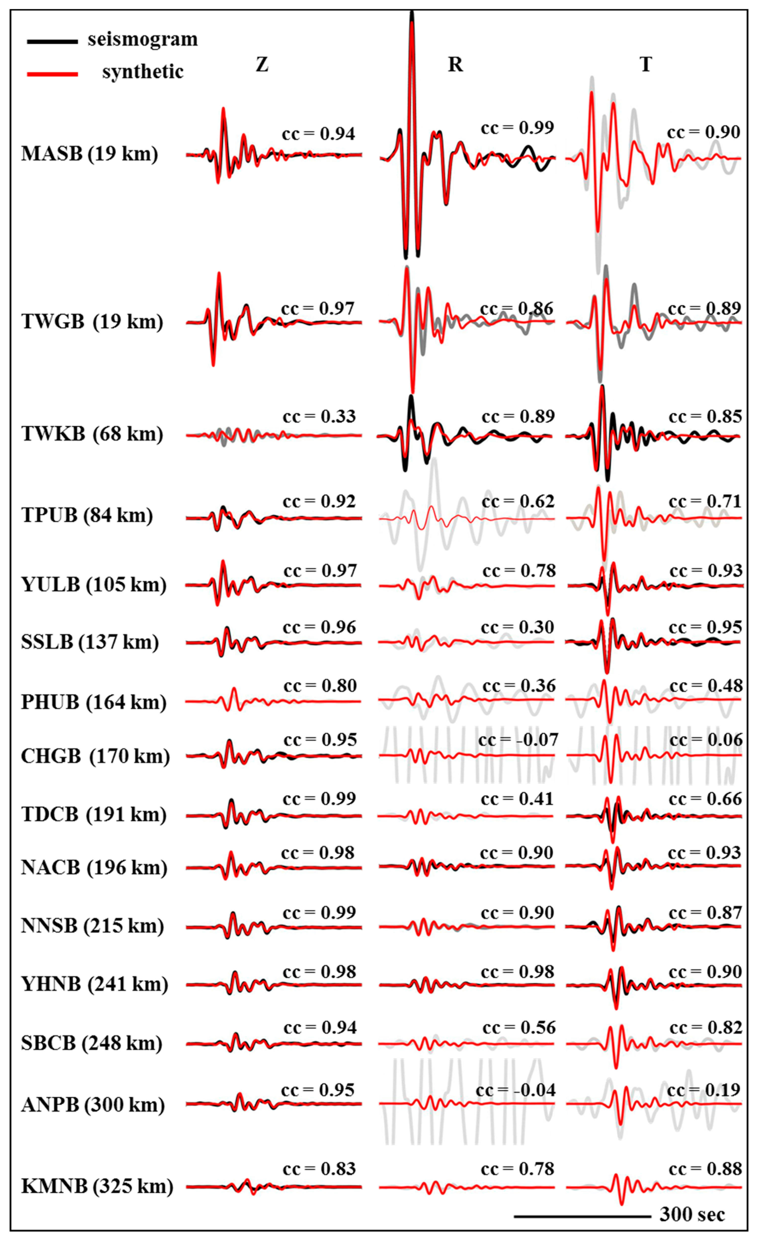
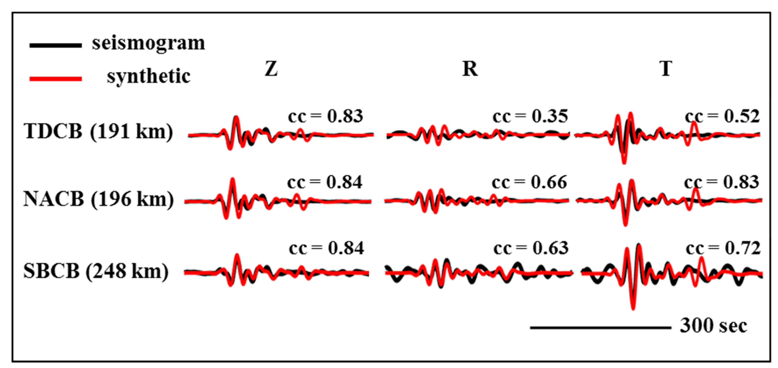
4.1. Results of PFH Inversion

The inversion results showed that the force induced by the Taimali landslide was initiated at about 09:31:34 and terminated at 09:34:28 (Figure 5). Among the three components of force, the largest force existed in the E–W direction, reaching 3.7 × 10¹⁰ N. The maximum force in the N–S direction and the maximum vertical forces were 1.6 × 10¹⁰ and 1.2 × 10¹⁰ N, respectively.

After the force–time function was obtained, the inverted force was applied to get the synthetic waveforms of each seismic station (Figure 6). Most synthetic waveforms were consistent with the station records: 47% of the synthetic waveforms had correlation coefficients (cc) values higher than 0.9, and 70% of the synthetic waveforms had cc values higher than 0.7. They both indicated that the inversion results were robust. The ANPB and CHGB stations both had strong ambient noise, which led to the low SNR and cc values. In addition, the poor results of the KMNB and PHUB stations might be attributable to the velocity model used in this study. Despite the poor results caused by the strong ambient noise and the influence of the velocity model, the high cc values suggested that the inversion had good performance and the results were highly reliable.

Based on the analysis of satellite imagery and the results of waveform inversion, the Taimali landslide slid toward the northeast at the beginning, which implied that the force would first head toward the southwest. However, the first pulse of force from 09:31:21 to 09:31:34 was toward the northeast. Thus, the first pulse of force was considered a precursory signal caused by Gibbs effects [7]. The landslide propagation began at 09:31:34, at which time the force headed toward the southwest. The force after the 250th second was considered fluctuations of ambient noise, not the propagation of the Taimali landslide. The 174-s duration of the landslide was consistent with the waveform observation (Figure 6); therefore, the force–time function indicated that the Taimali landslide initiated at 09:31:34 and terminated at 09:34:28.

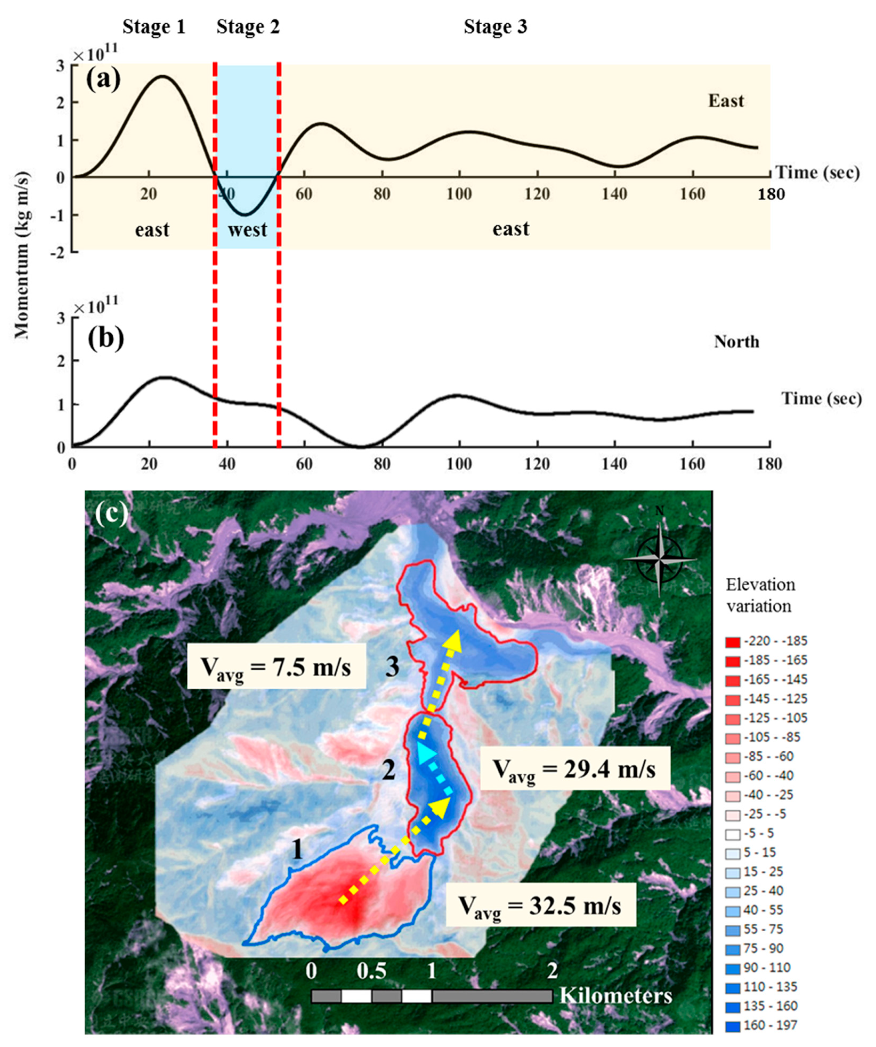
4.2. Dynamic Processes Determined by PFH Inversion

PFH inversion is based on the assumption that a landslide is a block having a constant mass m. With the constant landslide mass, the landslide momentum (m × v) can be calculated by integrating the force–time function. As the Taimali landslide first slid toward the northeast, the E–component momentum increased and reached the maximum at the 24th second (Figure 7a). After that, both the E- and N-component momentums decreased, and the E-component momentum reached zero; subsequently, the landslide turned to the west at the 37th second (Figure 7b). The time interval between the 1st and the 37th seconds (09:31:34–09:32:11) can be considered the first stage of the landslide propagation (Figure 7c).

The landslide slid toward the west for only a short time, i.e., 17 s, and turned to the east again. The time interval between the 37th and 54th seconds (09:32:11–09:32:28) can be considered the second stage of the landslide propagation (Figure 7c). After the 54th second (09:32:28), the landslide continued toward the east until it stopped. Therefore, the time interval between the 54th and 174th seconds (09:32:28–09:34:28) can be considered the third stage of the landslide propagation. The variations of velocity in the E- and N-components did not decrease to zero at the end of landslide propagation. Yamada et al. [14] noted that long-period noise might accumulate with linear trends as the force is integrated in the time domain. Meanwhile, the slight fluctuations in the momentums in the third stage were possibly caused by the small landslides around the Taimali landslide. During the third stage, some small landslides might have generated weak seismic signals that affected the inversion results. Besides, the trajectories of the landslide movement could be measured from the post-event satellite images and DEM. The starting point was defined at the deepest point of the landslide source area. There were two obvious topographic turning points on the route of the landslide movement. The turning points could be considered the starting points of the second and third stages. In addition, the centroid of the deposit area in the river channel could be considered the termination point of the landslide. Eventually, the runout distances of each stage and average velocities could be calculated (

Table 3. Three dynamic process stages of the Taimali landslide.

Stage	Duration (s)	Runout Distance (m)	Average Velocity (m/s)
1	37	1200	32.5
2	17	500	29.4
3	120	900	7.5

).

Chao et al. [16] performed a waveform inversion using the LFH method for the Taimali landslide. To ensure the equilibrium of forces, the LFH method makes strict assumptions about the force changes during the landslide (unloading/reloading cycles). As a result, the block trajectory deduced by the LFH inversion may not completely correspond to the real terrain, but can only show the overall direction of movement. The PFH method does not confine the force changes during a landslide within certain limits, so a more detailed force–time function can be obtained, which can be used to reflect the correlation between the landslide propagation and the actual terrain. Pan et al. [26] and Huang [27] used a 3D discrete element method to simulate the dynamic processes of the Taimali landslide. The studies both displayed that the landslide moved toward the northeast, which coincides with the results from the PFH inversion method. Besides, Huang [27] reported that the landslide turned to the west at the 40th second, and the movement velocity exceeded 20 m/s. Although the two numerical simulations did not present the force history of the landslide, the simulated movement direction and velocity were both consistent with the results of the PFH inversion method.

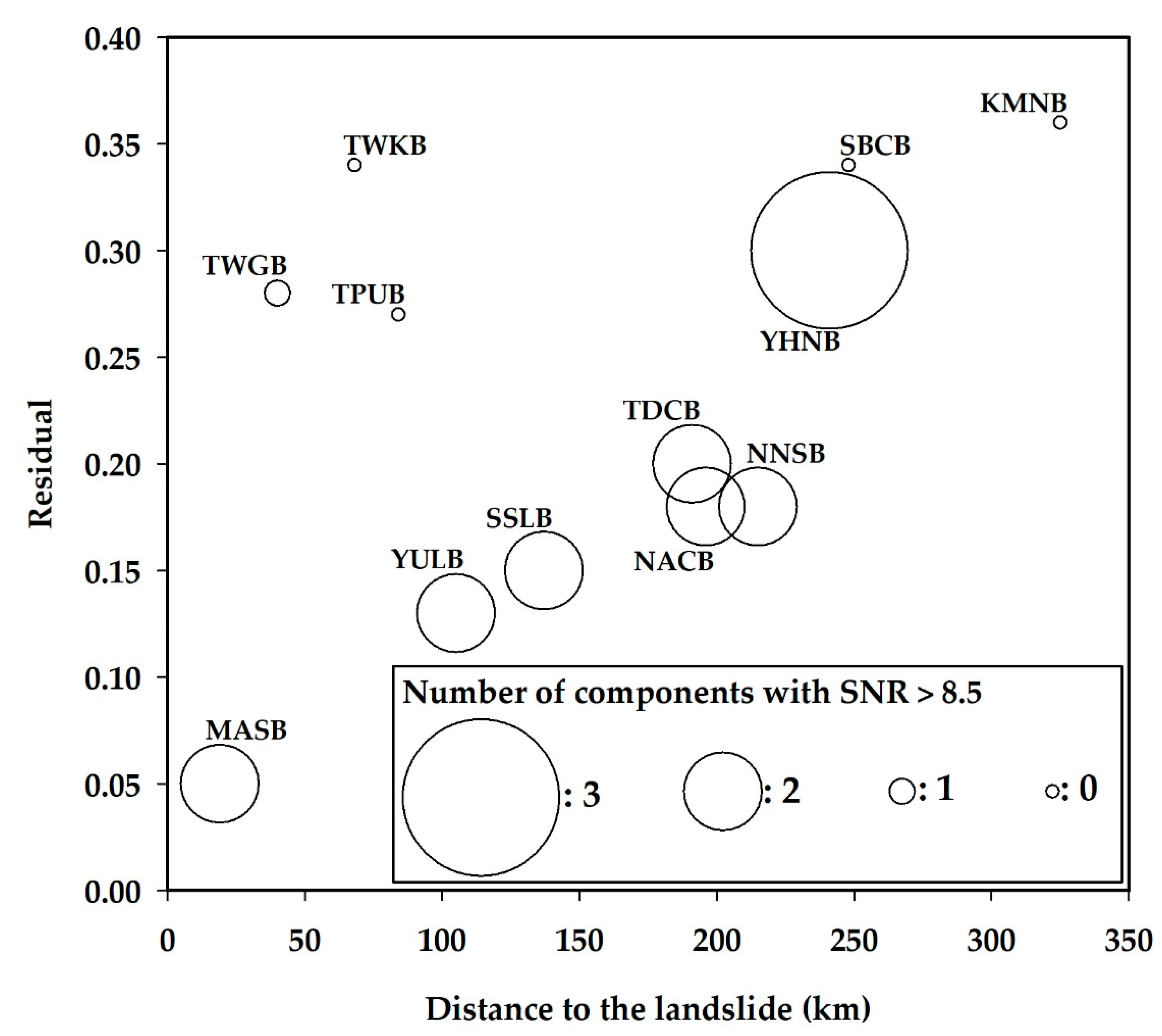
4.3. The Requirement for the Single-Station Inversion

In general, most waveform inversion methods are limited by the quality of the seismic data and the station coverage. The results of waveform inversion will be more robust if seismic records having high SNR values are used and station coverage is complete. It was particularly noteworthy that PFH inversion could be executed with high-quality seismic records from a single station. Accordingly, single-station waveform inversions were performed on each of the 15 station records. The residual of the M_LQ value between the multistation inversion and the single-station inversion was calculated to testify to the quality of the single-station inversion (

Table 4. The residuals between all-station inversion and single-station version.

Station	Distance (km)	R-SNR	T-SNR	Z-SNR	Residual
MASB	19	9.2	6.2	11.3	0.05
TWGB	40	7.3	6.5	9.5	0.28 *
TWKB	68	7	8.2	7.2	0.34 *
TPUB	84	3.9 #	7.3	7.4	0.27 *
YULB	105	6.8	10.5	10.4	0.13
SSLB	137	4.0 #	9	9.2	0.15
TDCB	191	3.3 #	9.9	10	0.20
NACB	196	7.6	11	10.4	0.18
NNSB	215	6.2	8.9	10.6	0.18
YHNB	241	7.7	10.2	10.3	0.30 *
SBCB	248	3.9 #	5.8	8.3	0.34 *
KMNB	325	6.7	7	6.7	0.36 *

^# SNR values less than 4. * residual values larger than 0.2.

). The M_LQ value was defined as the value of the landslide mass multiplied by the runout distance [17]. The results revealed that half of the single-station inversions had residuals below 0.2 and had fine consistency with the multistation inversion. It appeared that the seismic records having higher SNR values led to lower residuals and were more suitable for use in single-station inversion. The M_LQ value of the TWKB single-station inversion was overestimated and led to a high residual, which might have been caused by the environmental conditions of the seismometer or geological factors. The seismic amplitudes recorded by the TWKB station were abnormally high and unsuitable for single-station waveform inversion. Although the YHNB station had a high SNR value, the M_LQ value of the YHNB single-station inversion was underestimated, possibly due to its distance from the seismic source and to waveform attenuation. The rest of the high residuals of M_LQ occurred at the stations having low SNR values. In addition, the single-station inverted force can be applied to synthesize waveforms for other stations to acquire high correlation coefficients, which enhances the reliability of the single-station inversion (Figure 8).

The residuals between 15-station inversion and single-station inversion reveal that the errors caused by single-station inversion increase with station distance to the landslide (Figure 9). Once the residuals are considered as the errors, the MASB single-station inversion would cause an error of 5%, and result in a slight decrease of 0.1–0.15 in the correlation coefficients between the synthetic and observed waveforms. As the error caused by the single-station inversion is larger than 20% (e.g., YHNB, KMNB, etc.), the correlation coefficient between the synthetic and observed waveforms would decrease significantly to lower than 0.3. The noise level at each station is another factor to influence the waveform inversion. In Figure 9, we can observe that when the number of components with SNR > 8.5 is less than two, the errors of single-station inversion are larger than 20%. Moreover, the azimuthal coverage of the seismic network is not very dense; the azimuth gap is large especially in the east, which will influence the selection of seismic records. Therefore, we deduce that the quality of the seismic data and the station coverage are the main factors in determining the results of waveform inversion. In summary, we suggest that stations having SNR values higher than 8.5 and located within 200 km of a landslide are appropriate for use in single-station waveform inversion and may have residuals of M_LQ values below 0.2. The single-station PFH inversion provides a chance to analyze small-scale landslides. Small-scale landslides generate weak seismic signals and may not be detected by many seismic stations, making it difficult to constrain the results of the multistation waveform inversion. The dynamic processes of a landslide can still be extracted by executing single-station PFH inversion with high-SNR seismograms.

5. Conclusions

Waveform inversion techniques provide information for the study of the dynamic processes of a landslide. In this study, the Taimali landslide of 2009 was chosen for the implementation of waveform inversion using the PFH method. According to the pre- and post-event DEMs, the source area of the Taimali landslide had an area of 9.3 × 10⁵ m² and a volume of 7.5 × 10⁷ m³. PFH inversion presented the complicated force–time functions and two impact timings during the propagation of the landslide. Thus, the 174-s total of the dynamic processes can be divided into three stages for the different sliding directions: northeast for the first stage, northwest for the second stage, and northeast for the third stage. The average sliding velocities of the three stages were 32.5, 29.4, and 7.5 m/s, respectively. The inversion results indicated that the PFH inversion method could extract the dynamic processes of the landslide, even if the directions of landslide movement varied during propagation. The study also proved that the single-station waveform inversion was feasible by using the PFH inversion method with high-quality seismic data.

References

1. Huang, S.W.; Jean, J.S.; Hu, J.C. Huge rock eruption caused by the 1999 Chi-Chi earthquake in Taiwan. Geophys. Res. Lett. 2003, 30, 1858. [Google Scholar] [CrossRef]
2. Yu, F.C.; Chen, L.K. Discussion on slope disasters triggered by Typhoon Morakot. J. Civil Hydraul. Eng. 2010, 37, 32–40. (In Chinese) [Google Scholar]
3. Council of Agriculture. Typhoon Morakot: An overview of agriculture loss. In Agriculture Policies and Circumstances; Council of Agriculture, Executive Yuan: Taipei, Taiwan, 2009; p. 207. (In Chinese) [Google Scholar]
4. Chigira, M. The Potential Area of Large-Scale Landslides; Scientific & Technical Publishing Co., Ltd.: Taipei, Taiwan, 2011. (In Chinese) [Google Scholar]
5. Hibert, C.; Ekström, G.; Stark, C.P. Dynamics of the Bingham Canyon Mine landslides from seismic signal analysis. Geophys. Res. Lett. 2014, 41, 4535–4541. [Google Scholar] [CrossRef]
6. Brodsky, E.E.; Gordeev, E.; Kanamori, H. Landslide basal friction as measured by seismic waves. Geophys. Res. Lett. 2003, 30, 2236. [Google Scholar] [CrossRef]
7. Ekström, G.; Stark, C.P. Simple scaling of catastrophic landslide dynamics. Science 2013, 339, 1416–1419. [Google Scholar] [CrossRef] [PubMed]
8. Lin, C.H.; Jan, J.C.; Pu, H.C.; Tu, Y.; Chen, C.C.; Wu, Y.M. Landslide seismic magnitude. Earth Planet. Sci Lett. 2015, 429, 122–127. [Google Scholar] [CrossRef]
9. Fan, X.; Scaringi, G.; Dai, L.; Li, W.; Dong, X.; Zhu, X.; Pei, X.; Dai, K.; Havenith, H. Failure mechanism and kinematics of the deadly June 24th 2017 Xinmo landslide, Maoxian, Sichuan, China. Landslides 2017, 14, 2129–2146. [Google Scholar] [CrossRef]
10. Kanamori, H.; Given, J.W. Analysis of long-period seismic waves excited by the May 18, 1980, eruption of Mount St. Helens—A terrestrial monopole? J. Geophys. Res. Solid Earth 1982, 87, 5422–5432. [Google Scholar] [CrossRef]
11. Kanamori, H.; Given, J.W.; Lay, T. Analysis of seismic body waves excited by the Mount St. Helens eruption of May 18, 1980. J. Geophys. Res. Solid Earth 1984, 89, 1856–1866. [Google Scholar] [CrossRef]
12. Nakano, M.; Kumagai, H.; Inoue, H. Waveform inversion in the frequency domain for the simultaneous determination of earthquake source mechanism and moment function. Geophys. J. Int. 2018, 173, 1000–1011. [Google Scholar] [CrossRef]
13. Lin, C.H.; Kumagai, H.; Ando, M.; Shin, T.C. Detection of landslides and submarine slumps using broadband seismic networks. Geophys. Res. Lett. 2010, 37, L22309. [Google Scholar] [CrossRef]
14. Yamada, M.; Kumagai, H.; Matsushi, Y.; Matsuzawa, T. Dynamic landslide processes revealed by broadband seismic records. Geophys. Res. Lett. 2013, 40, 2998–3002. [Google Scholar] [CrossRef]
15. Hibert, C.; Stark, C.P.; Ekström, G. Dynamics of the Oso-Steelhead landslide from broadband seismic analysis. Nat. Hazards Earth Syst. Sci. 2015, 15, 1265–1273. [Google Scholar] [CrossRef]
16. Chao, W.A.; Zhao, L.; Chen, S.C.; Wu, Y.M.; Chen, C.H.; Huang, H.H. Seismology-based early identification of dam-formation landquake events. Sci. Rep. 2016, 6, 19259. [Google Scholar] [CrossRef] [PubMed]
17. Allstadt, K. Extracting source characteristics and dynamics of the August 2010 Mount Meager landslide from broadband seismograms. J. Geophys. Res. Earth Surf. 2013, 118, 1472–1490. [Google Scholar] [CrossRef]
18. Iverson, R.M.; George, D.L.; Allstadt, K.; Reid, M.E.; Collins, B.D.; Vallance, J.W.; Schilling, S.P.; Godt, J.W.; Cannon, C.M.; Magirl, C.S.; et al. Landslide mobility and hazards: Implications of the 2014 Oso disaster. Earth Planet. Sci. Lett. 2015, 412, 197–208. [Google Scholar] [CrossRef]
19. Kuo, H.L. A Study of Landslide-Triggering Rainfall Conditions by Analyzing the Ground Motion Signals Induced by Large-Scale Landslides. Master’s Thesis, National Cheng Kung University, Tainan, Taiwan, 2016; 139p. (In Chinese). [Google Scholar]
20. Wang, Y.C.; Chen, W.F. Study on Damages Analysis and Improvement Programs of Flood Control Structures Caused by Compound Disasters after Typhoon Morokot—Taimali River as an Example. In Chinese Soil and Water Conservation Society Conference and Academic Seminar Abstracts; Chinese Soil and Water Conservation Society: Taipei, Taiwan, 2012; 16p. [Google Scholar]
21. Ho, C.S. An introduction to The Geology of Taiwan Explanatory Text of The Geologic Map of Taiwan; Central Geological Survey: Taipei, Taiwan, 1994. (In Chinese)
22. IES. Broadband Array in Taiwan for Seismology; Other/Seismic Network; Institute of Earth Sciences, Academia Sinica: Taipei, Taiwan, 1996. [Google Scholar] [CrossRef]
23. Eissler, H.K.; Kanamori, H. A single-force model for the 1975 Kalapana, Hawaii, earthquake. J. Geophys. Res. Solid Earth 1987, 92, 4827–4836. [Google Scholar] [CrossRef]
24. Herrmann, R.B. Computer Programs in Seismology: An Overview of Synthetic Seismogram Computation; Saint-Louis University: St. Louis, MO, USA, 2002. [Google Scholar]
25. Chen, Y.L.; Shin, T.C. Study on the earthquake location of 3-D velocity structure in the Taiwan area. Meteorol. Bull. 1998, 42, 135–169. [Google Scholar]
26. Pan, Y.W.; Su, H.K.; Liao, J.J.; Huang, M.W. Reconstruction of rainfall-induced landslide dam by numerical simulation-the Barrier Lake in Taimali River as an example. In Rock Mechanics for Global Issues, Proceedings of the ISRM International Symposium-8th Asian Rock Mechanics Symposium, Sapporo, Japan, 14–16 October 2014; International Society for Rock Mechanics and Rock Engineering: Lisbon, Portugal, 2014. [Google Scholar]
27. Huang, C.M. Combination of Three-Dimensional Discrete Element Method and Geological Model to Simulate the Migration of Taimali Landslide, Xinmo Landslide and Shezailiao Landslide-Prone Slope. Master’s Thesis, National Cheng Kung University, Tainan, Taiwan, 2019. (In Chinese). [Google Scholar]
Figure 1. The location of the study area. (a) The location of the Taimali landslide and the distribution of 15 seismic stations adopted in the waveform inversion. (b) The post-event satellite image of the Taimali landslide. The blue line denotes the boundary of the source area.
Applsci 10 05872 g001
Figure 2. The map of the source area and the deposit areas of the Taimali landslide. The source area is marked by the blue line. The deposit areas are marked by red lines.
Applsci 10 05872 g002
Figure 3. Original displacement seismographs of the Taimali landslide.
Applsci 10 05872 g003
Figure 4. Vertical seismic signal of the Taimali landslide recorded at the MASB station. (a) Original waveform, (b) spectrogram, (c) spectrum, (d) 0.01–0.033 Hz filtered waveform, and (e) 1–5 Hz filtered waveform. The signal recording begins at local time 2009–08–09 16:31:00 and the sampling rate is 20 Hz.
Applsci 10 05872 g004
Figure 5. The force–time function of the Taimali landslide by point force history (PFH) method. The time series began at 09:31 and ended at 09:36 UTC. The green zone represents the duration of the landslide propagation.
Applsci 10 05872 g005
Figure 6. Three components of the synthetic waveforms and the seismograms of each station. Z denots vertical direction, R denotes radial direction, and T denotes tangential direction. Correlation coefficients are represented by “cc”. Light-colored seismograms represent that the lower weighted coefficients were adopted to conduct the PFH inversion.
Applsci 10 05872 g006
Figure 7. Dynamic run-out direction of the Taimali landslide. (a) The momentum changes in the eastern direction. Notice that the start time was 09:31:34, which is the 34th second in Figure 3. (b) The momentum changes in the north direction. (c) The three landslide propagation stages and the average velocity for each stage.
Applsci 10 05872 g007
Figure 8. The synthetic waveforms of the TDCB, NACB, and SBCB stations by the MASB single-station inverted force (red curves) and observed records (black curves).
Applsci 10 05872 g008
Figure 9. The correlation between distance to the landslide and residual of single-station inversion.
Applsci 10 05872 g009