Robust Path Tracking Control for Autonomous Vehicle Based on a Novel Fault Tolerant Adaptive Model Predictive Control Algorithm


Abstract
:1. Introduction
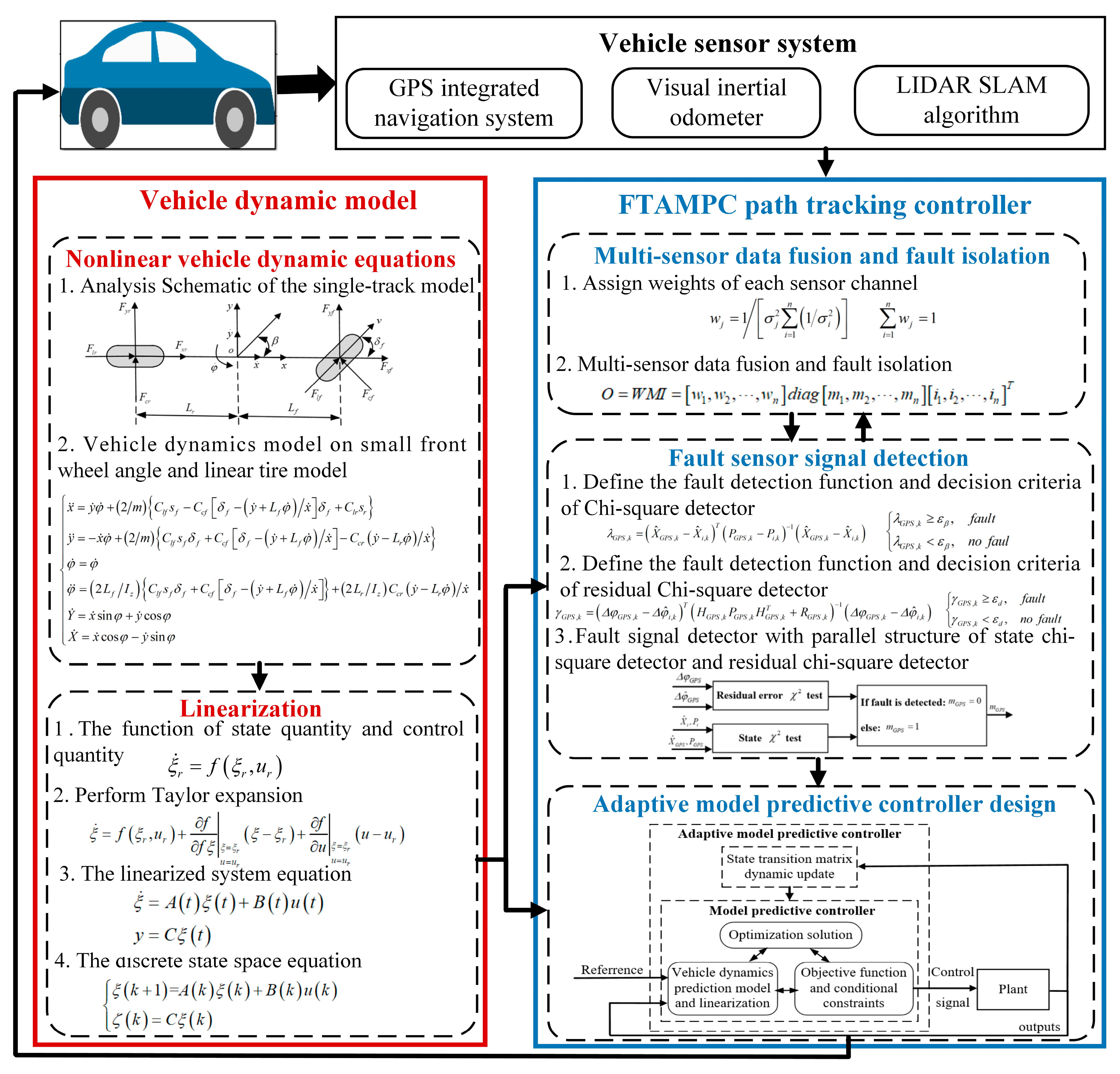
2. Methodology
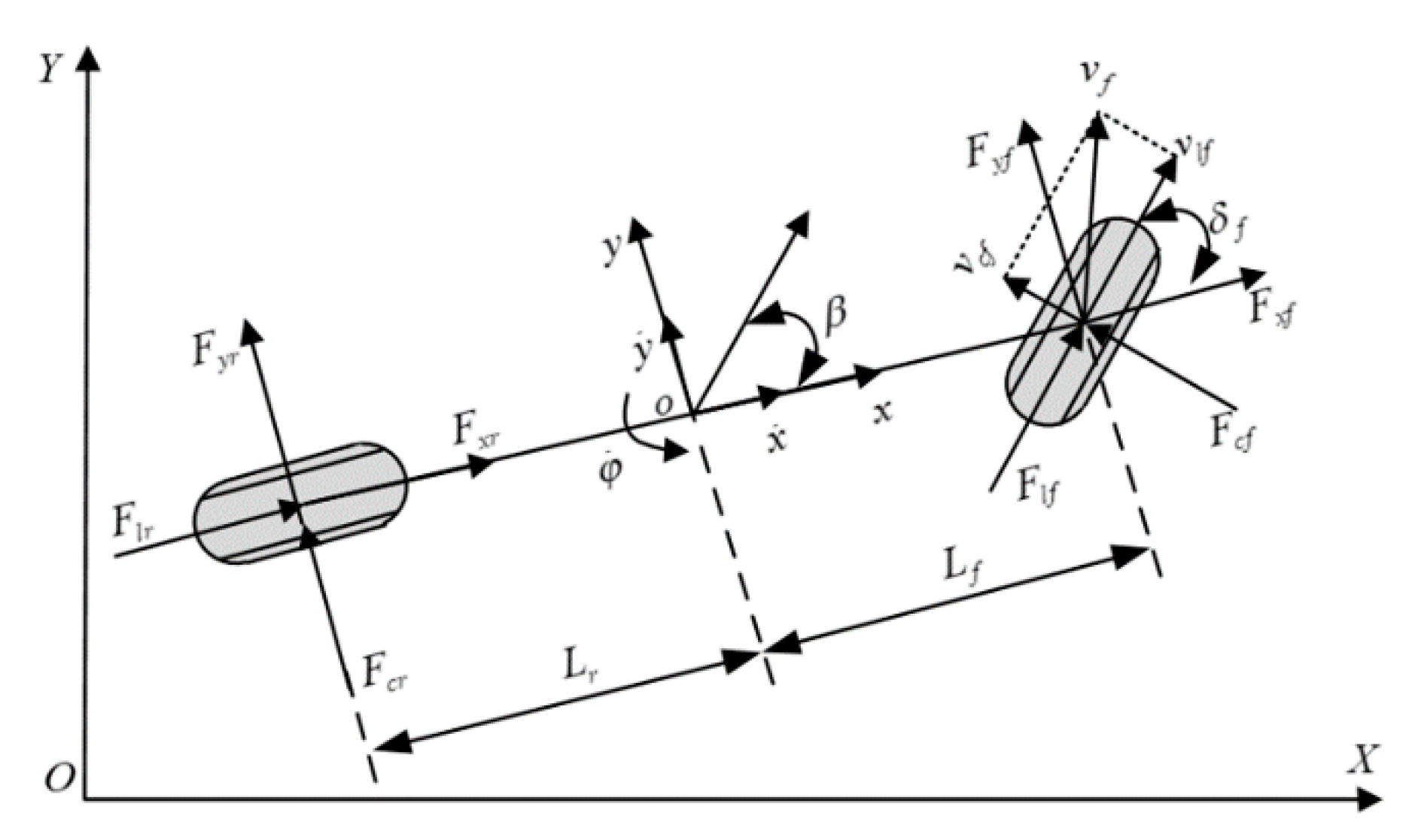
2.1. Modeling and Problem Formulation
2.2. Linearization of Vehicle Dynamics Model
2.3. Construct the Constraints
2.4. Dynamic Constraint of Tire Cornering
2.5. Lateral Acceleration Constraints
2.6. Construct the Objective Function
2.7. Adaptive Model Predictive Controller for Vehicle Lateral Motion Control
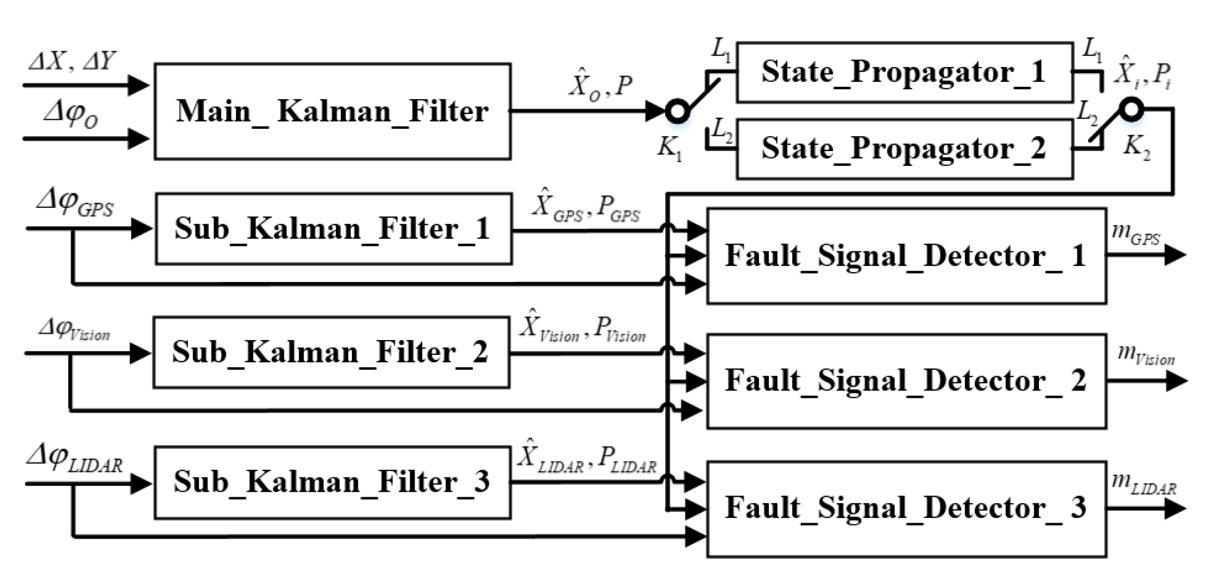
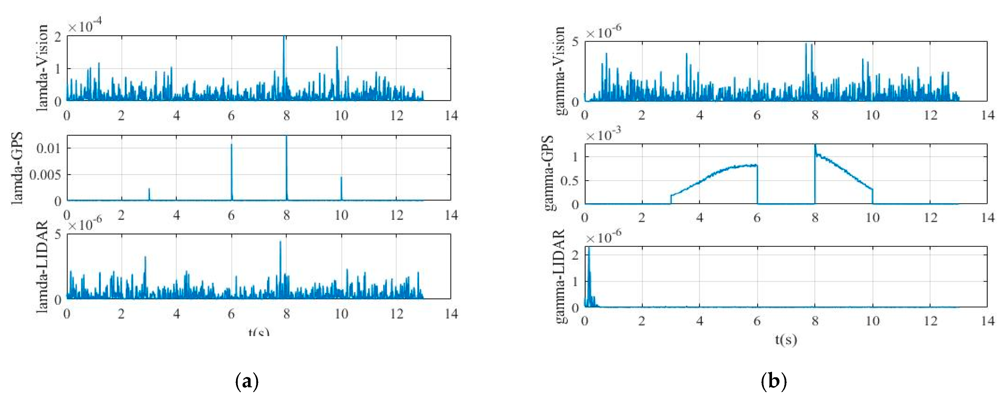
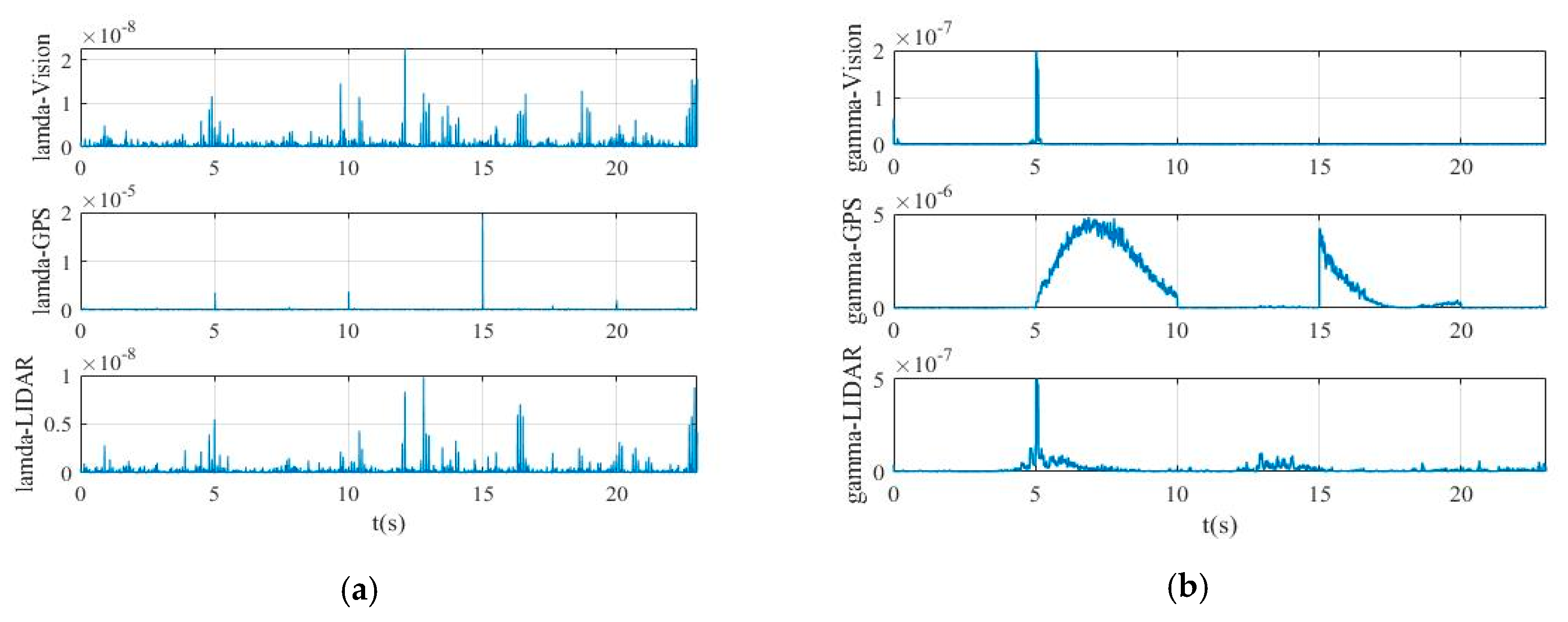
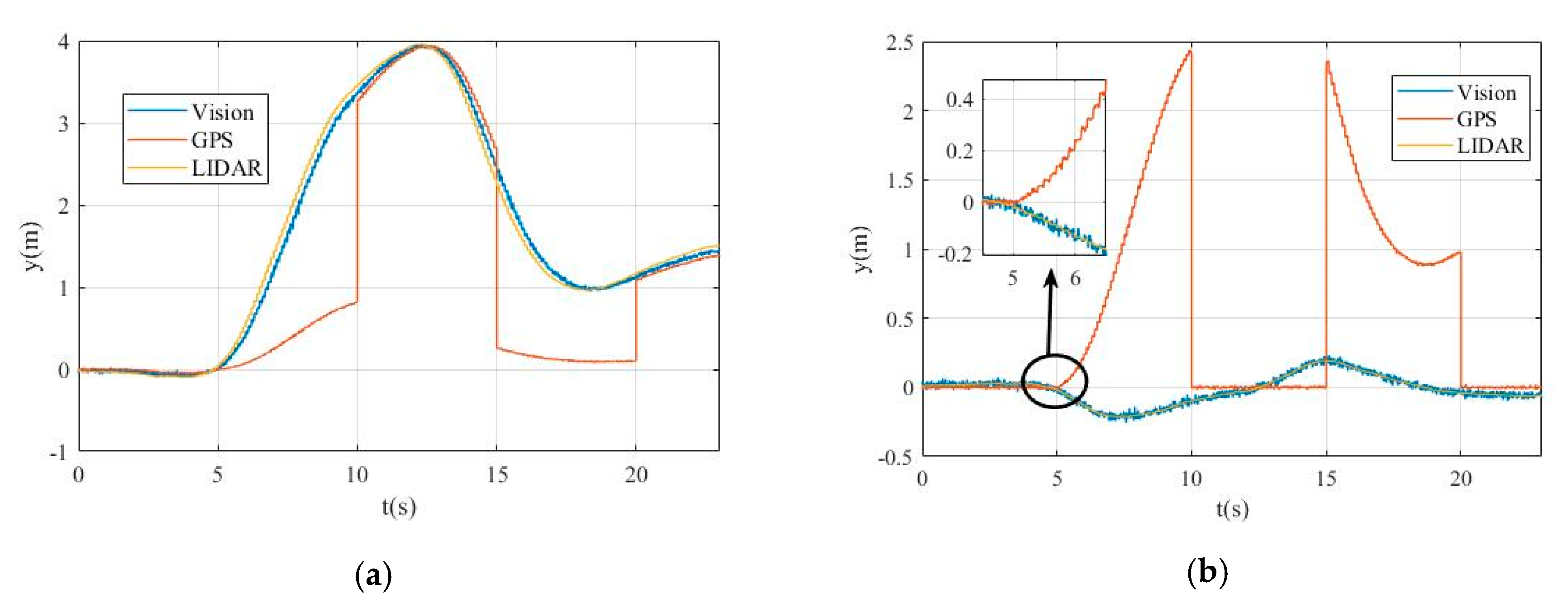
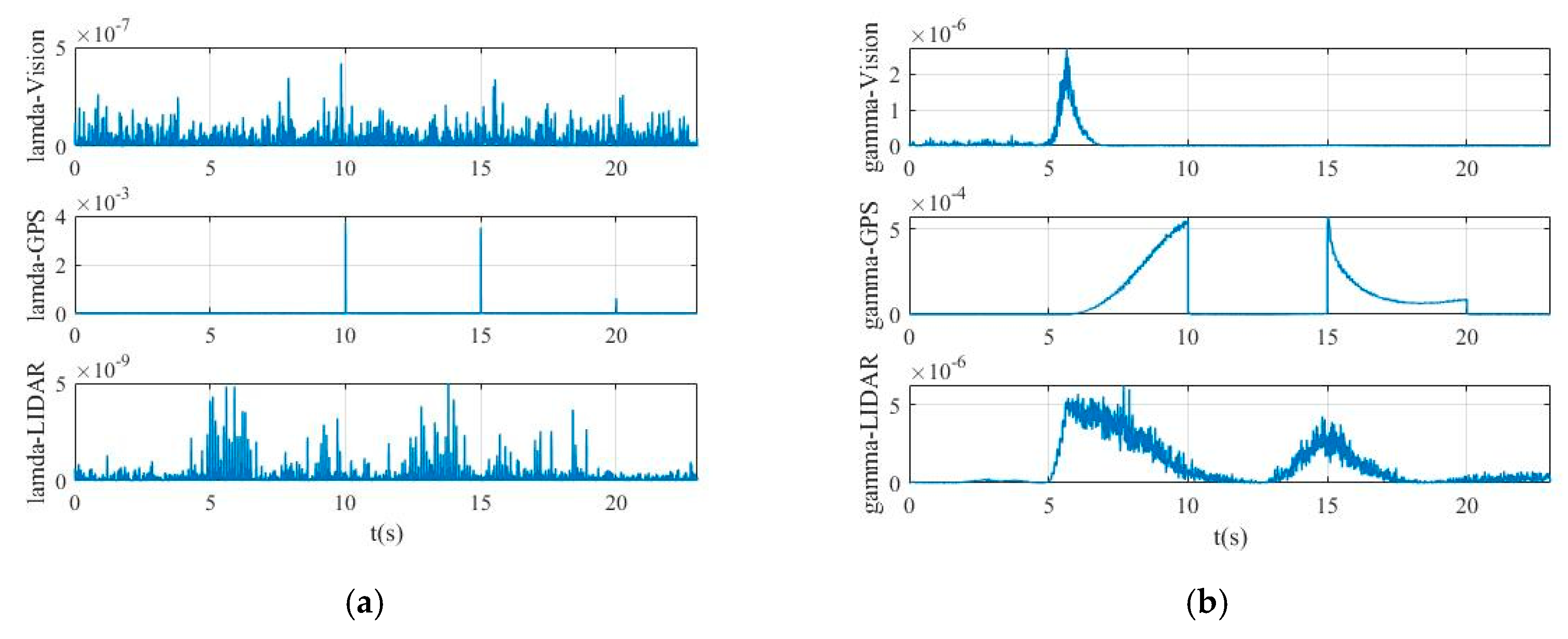
2.8. Merging Multi-Sensor Data and Isolating Fault Signals
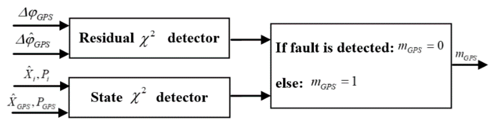
2.9. Fault Signal Detector Design
3. Results
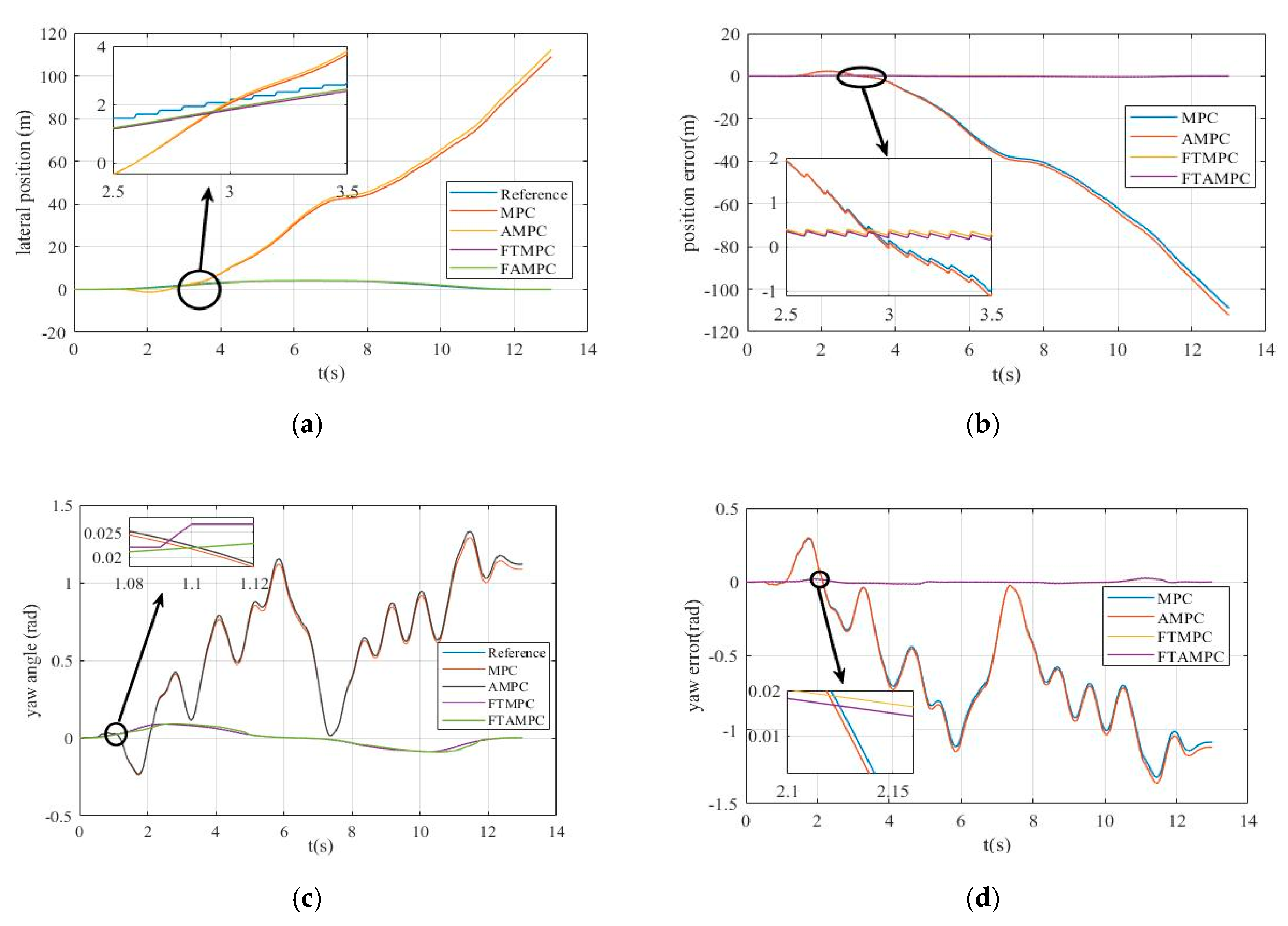
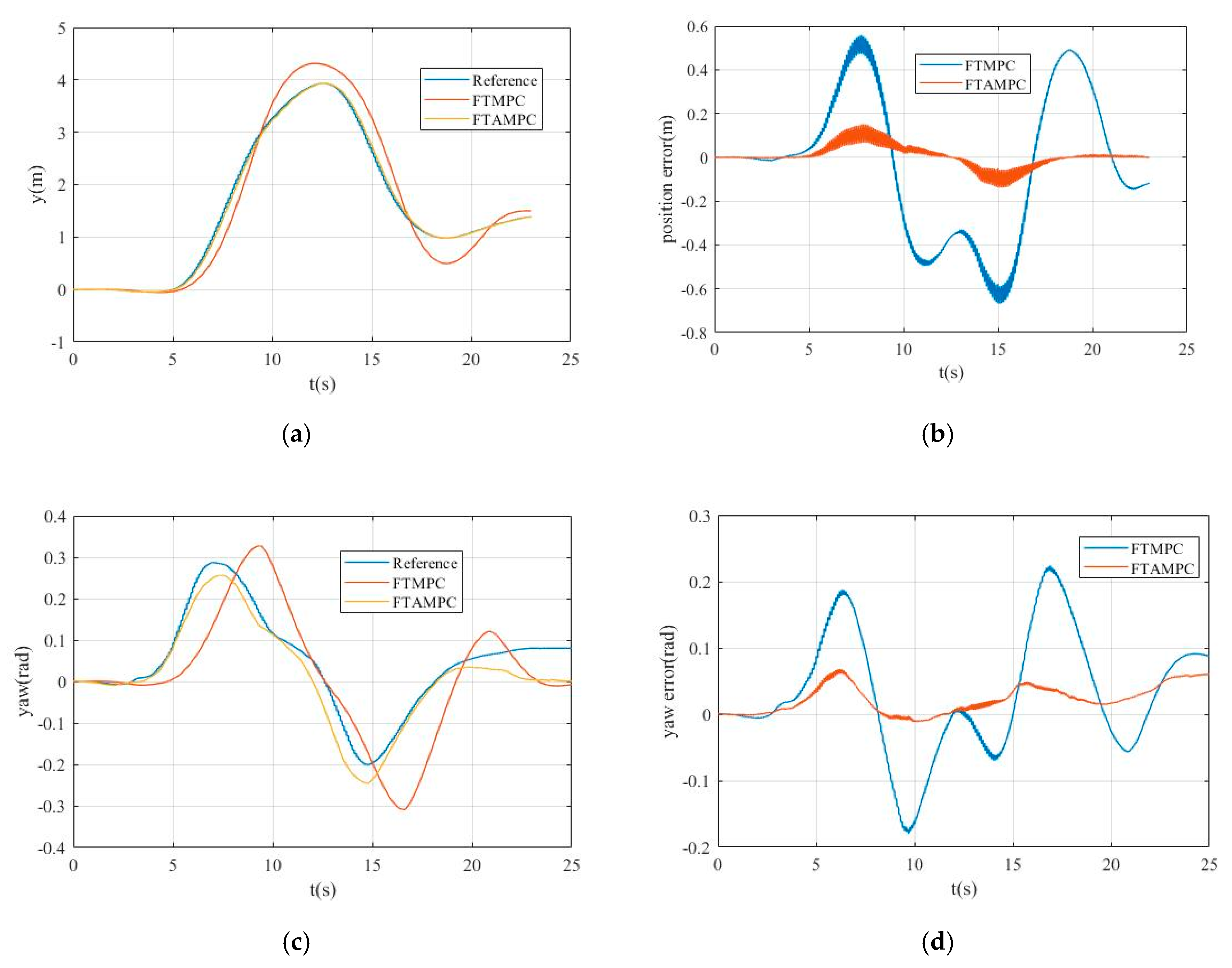
3.1. Simulation Verification
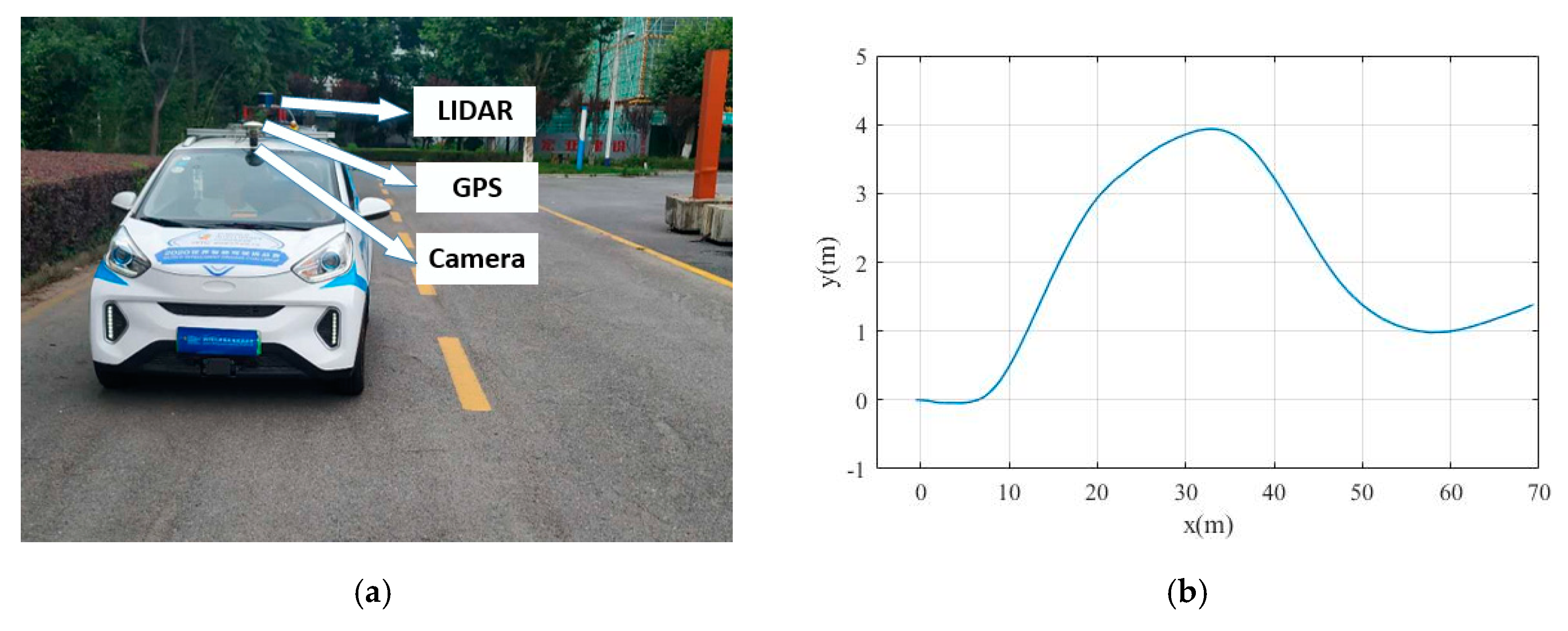
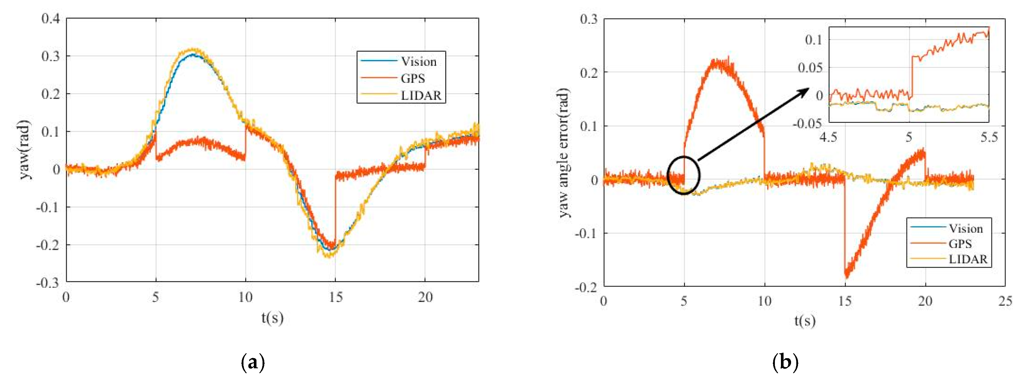
3.2. Experimental Verification
4. Conclusions
Author Contributions
Funding
Conflicts of Interest
References
- Kim, M.-H.; Lee, S.; Ha, K.-N.; Lee, K.-C. Implementation of a fuzzy-inference-based, low-speed, close-range collision-warning system for urban areas. Proc. Inst. Mech. Eng. Part D J. Automob. Eng. 2012, 227, 234–245. [Google Scholar] [CrossRef]
- Cui, Q.; Ding, R.; Zhou, B.; Wu, X. Path-tracking of an autonomous vehicle via model predictive control and nonlinear filtering. Proc. Inst. Mech. Eng. Part D J. Automob. Eng. 2017, 232, 1237–1252. [Google Scholar] [CrossRef]
- Wang, R.; Jing, H.; Hu, C.; Yan, F.; Chen, N. Robust H∞ path following control for autonomous ground vehicles with delay and data dropout. IEEE Trans. Intell. Transp. Syst. 2016, 17, 2042–2050. [Google Scholar] [CrossRef]
- Xia, Y.; Pu, F.; Li, S.; Gao, Y. Lateral path tracking control of autonomous land vehicle based on ADRC and differential flatness. IEEE Trans. Ind. Electron. 2016, 63, 3091–3099. [Google Scholar] [CrossRef]
- Xu, S.; Peng, H. Design, analysis, and experiments of preview path tracking control for autonomous vehicles. IEEE Trans. Intell. Transp. Syst. 2019, 21, 48–58. [Google Scholar] [CrossRef]
- Checkoway, S.; Mccoy, D.; Anderson, D. Comprehensive experimental analyses of automotive attack surfaces. In Proceedings of the 21st Usenix Security Symposium, Bellevue, WA, USA, 6–7 August 2012; USENIX Association: Berkeley, CA, USA, 2012. [Google Scholar]
- Realpe, M.; Vintimilla, B.X.; Vlacic, L. Sensor fault detection and diagnosis for autonomous vehicles. MATEC Web Conf. 2015, 30, 4003. [Google Scholar] [CrossRef] [Green Version]
- Nicolas, P.; Denis, G.; Dominique, G. Intelligent vehicle embedded sensors fault detection and identification using analytical redundancy and non-linear transformations. J. Control Sci. Eng. 2017, 2017, 1763934. [Google Scholar]
- Darms, M.; Rybski, P.; Urmson, C. Classification and tracking of dynamic objects with multiple sensors for autonomous driving in urban environments. In Proceedings of the 2008 IEEE Intelligent Vehicles Symposium, Eindhoven, The Netherlands, 4–6 June 2008; pp. 1197–1202. [Google Scholar] [CrossRef] [Green Version]
- Yang, S.; Liu, Z.; Li, J.; Wang, S. Anomaly detection for internet of vehicles: A trust management scheme with affinity propagation. Mob. Inf. Syst. 2016, 2016, 1–10. [Google Scholar] [CrossRef] [Green Version]
- Lin, R.; Khalastchi, E.; Kaminka, G.A. Detecting anomalies in unmanned vehicles using the Mahalanobis distance. In Proceedings of the 2010 IEEE International Conference on Robotics and Automation, Anchorage, AK, USA, 3–8 May 2010; pp. 3038–3044. [Google Scholar] [CrossRef]
- Khalastchi, E.; Kaminka, G.A.; Kalech, M. Anomaly detection in unmanned vehicles. In Proceedings of the International Conference on Autonomous Agents & Multiagent Systems—Volume 1, Taipei, Taiwan, 2–6 May 2011. [Google Scholar]
- Park, J.; Ivanov, R.; Weimer, J.; Pajic, M.; Lee, I. Sensor attack detection in the presence of transient faults. In Proceedings of the ACM/IEEE Sixth International Conference on Cyber-Physical Systems—ICCPS ’15, Seattle, WA, USA, 14–16 April 2015; Association for Computing Machinery (ACM): New York, NY, USA, 2015. [Google Scholar]
- Foo, G.H.B.; Zhang, X.; Vilathgamuwa, D.M. A sensor fault detection and isolation method in interior permanent-magnet synchronous motor drives based on an extended Kalman filter. IEEE Trans. Ind. Electron. 2013, 60, 3485–3495. [Google Scholar] [CrossRef]
- Wei, X.; Verhaegen, M.; Van Engelen, T. Sensor fault detection and isolation for wind turbines based on subspace identification and Kalman filter techniques. Int. J. Adapt. Control. Signal Process. 2009, 24. [Google Scholar] [CrossRef]
- Schmidhuber, J. Deep learning in neural networks: An overview. Neural Netw. 2015, 61, 85–117. [Google Scholar] [CrossRef] [PubMed] [Green Version]
- Malhotra, P.; Vig, L.; Shroff, G. Long short term memory networks for anomaly detection in time series. In Proceedings of the 23rd European Symposium on Artificial Neural Networks, Computational Intelligence and Machine Learning, ESANN 2015, Bruges, Belgium, 22–24 April 2015. [Google Scholar]
- Christiansen, P.; Nielsen, L.N.; Steen, K.A.; Jørgensen, R.N.; Karstoft, H. Deep anomaly: Combining background subtraction and deep learning for detecting obstacles and anomalies in an agricultural field. Sensors 2016, 16, 1904. [Google Scholar] [CrossRef] [PubMed] [Green Version]
- Min-Joo, K.; Je-Won, K.; Tieqiao, T. Intrusion detection system using deep neural network for in-vehicle network security. PLoS ONE 2016, 11, e0155781. [Google Scholar]
- Bezemskij, A.; Loukas, G.; Gan, D.; Anthony, R.J. Detecting cyber-physical threats in an autonomous robotic vehicle using bayesian networks. In Proceedings of the 2017 IEEE International Conference on Internet of Things (iThings) and IEEE Green Computing and Communications (GreenCom) and IEEE Cyber, Physical and Social Computing (CPSCom) and IEEE Smart Data (SmartData), Exeter, UK, 21–23 June 2017; pp. 98–103. [Google Scholar] [CrossRef]
- Muter, M.; Asaj, N. Entropy-based anomaly detection for in-vehicle networks. In Proceedings of the 2011 IEEE Intelligent Vehicles Symposium (IV), Baden-Baden, Germany, 5–9 June 2011; pp. 1110–1115. [Google Scholar] [CrossRef]
- Dai, Y.; Yu, S.; Yan, Y.; Yu, X. An EKF-based fast tube MPC scheme for moving target tracking of a redundant underwater vehicle-manipulator system. IEEE/ASME Trans. Mechatron. 2019, 24, 2803–2814. [Google Scholar] [CrossRef]
- Li, Y.; Sun, D.; Zhao, M.; Chen, J.; Liu, Z.; Cheng, S.L.; Chen, T. MPC-based switched driving model for human vehicle co-piloting considering human factors. Transp. Res. Part C Emerg. Technol. 2020, 115, 102612. [Google Scholar] [CrossRef]
- Zhou, G.; Wang, Y.; Du, H. A generalized method for three-dimensional dynamic analysis of a full-vehicle model. Proc. Inst. Mech. Eng. Part D J. Automob. Eng. 2020, 2020. [Google Scholar] [CrossRef]
- Kuhne, F.; Lages, W.F. Model Predictive Control of a Mobile Robot Using Linearization. Available online: http://www.ece.ufrgs.br/~fetter/mechrob04_553.pdf (accessed on 21 June 2020).
- Da, R. Failure detection of dynamical systems with the state chi-square test. J. Guid. Control Dyn. 1994, 17, 271–277. [Google Scholar] [CrossRef]

| Hardware | Property |
|---|---|
| Laser LIDAR: HESAI Pandar 40 | Lines: 40; Range: 200 m; Angular resolution: 0.1°; Updating: 20 Hz; Accuracy: ±2 cm |
| Radar: Delphi ESR | Range: 100 m; Viewing field: ±10 deg; Updating: 20 Hz; Accuracy: ±5 cm, ±0.12 m/s, ±0.5° |
| Navigation system: NovAtel SPAN-CPT | Accuracy: ±1 cm, ±0.02 m/s, ±0.05° (Pitch/Roll), 0.1° (Azimuth); Updating: 10 Hz |
| Camera: SY8031 | Resolution: 3264 × 2448; FPS: 15;Viewing field: 65° (vertical), 50° (horizontal) |
| Image processer: NVIDIA JTX 2 | CPU: ARM Cortex-A57 (Quad-core, 2 GHz); GPU: Pascal TM (256 core, 1300 MHz); RAM: LPDDR4 (8 G, 1866 MHz, 58.3 GB/s) |
| Controller: ARK-3520P | CPU: Intel Core i5-6440EQ (Quad-core, 2.8 GHz); RAM: LPDDR4 (32 G, 2133 MHz, 100 GB/s) |
© 2020 by the authors. Licensee MDPI, Basel, Switzerland. This article is an open access article distributed under the terms and conditions of the Creative Commons Attribution (CC BY) license (http://creativecommons.org/licenses/by/4.0/).
Share and Cite
Geng, K.; Liu, S. Robust Path Tracking Control for Autonomous Vehicle Based on a Novel Fault Tolerant Adaptive Model Predictive Control Algorithm. Appl. Sci. 2020, 10, 6249. https://doi.org/10.3390/app10186249
Geng K, Liu S. Robust Path Tracking Control for Autonomous Vehicle Based on a Novel Fault Tolerant Adaptive Model Predictive Control Algorithm. Applied Sciences. 2020; 10(18):6249. https://doi.org/10.3390/app10186249
Chicago/Turabian StyleGeng, Keke, and Shuaipeng Liu. 2020. "Robust Path Tracking Control for Autonomous Vehicle Based on a Novel Fault Tolerant Adaptive Model Predictive Control Algorithm" Applied Sciences 10, no. 18: 6249. https://doi.org/10.3390/app10186249