Article

Infrared Image Adaptive Enhancement Guided by Energy of Gradient Transformation and Multiscale Image Fusion

1
Key Laboratory of Optical Engineering, Institute of Optics and Electronics, Chinese Academy of Sciences, No.1, Optoelectronic Avenue, Wenxing Town, Shuangliu District, Chengdu 610209, China
2
University of Chinese Academy of Sciences, Beijing 100039, China
3
Systems Engineering Research Institute, Beijing 100036, China
*
Author to whom correspondence should be addressed.
Appl. Sci. 2020, 10(18), 6262; https://doi.org/10.3390/app10186262
Submission received: 21 July 2020 / Revised: 24 August 2020 / Accepted: 26 August 2020 / Published: 9 September 2020
(This article belongs to the Special Issue Infrared Imaging and NDT)

Abstract

:
The detail enhancement and dynamic range compression of infrared (IR) images is an important issue and a necessary practical application in the domain of IR image processing. This paper provides a novel approach to displaying high dynamic range infrared images on common display equipment with appropriate contrast and clear detail information. The steps are chiefly as follows. First, in order to protect the weak global details in different regions of the image, we adjust the original normalized image into multiple brightness levels by adaptive Gamma transformation. Second, each brightness image is decomposed into a base layer and several detail layers by the multiscale guided filter. Details in each image are enhanced separately. Third, to obtain the image with global details of the input image, enhanced images in each brightness are fused together. Last, we filter out the outliers and adjust the dynamic range before outputting the image. Compared with other conventional or cutting-edge methods, the experimental results demonstrate that the proposed approach is effective and robust in dynamic range compression and detail information enhancement of IR image.

1. Introduction

The infrared sensor can capture the thermal radiation emitted by the objects, which is less impacted by the dark condition. It is widely applied in detection, scene surveillance, reconnaissance, and navigation, etc. due to its ability to operate 24 h a day. However, IR images do have many obvious shortcomings, including low contrast, weak details, and blurred resolution, when compared with visible images, which may trigger much inconvenience when people observe the images. Consequently, infrared sensors in high dynamic range (>8 bit) are always applied in practical application to capture more details in these years. If displaying the HDR images on normal facilities (8 bit) directly, some information in the original image could not be represented. The procedure to achieve high-quality visualization of HDR infrared image must take the following problems into consideration. First and foremost, the dynamic range of the output should be mapped to be acceptable for the display device. Meanwhile, in order to take advantage of the HDR sensor and guarantee convenience for the following work, weak details should be enhanced. Last but not least, the output should be as visually pleasing as possible.
The core idea of many conventional approaches is adjusting the distribution of the gray level. Those methods usually include linear stretching and curve stretching (logarithmic, gamma, and sigmoid) methods based on histogram equalization [1] (HE) and gradient domain methods.
Linear stretching can compress the dynamic range to be acceptable for the display equipment, while it leads to detail losing. Curve stretching like Gamma transformations can increase the image contrast, while the fitting parameters change when the images are different. For each image, manual selection of parameters with experience is required.
HE enlarges the contrast of the image by redistributing the image pixel values so that the number of pixels in each gray level is approximately equal. Researchers have made plenty of efforts based on HE [2,3,4,5,6,7,8], including global HE-based approaches and local HE-based approaches. The global HE-based approaches like Plateau HE [3,4] and its improved ones [2,7] can make the gray levels distribute more reasonably, but the ability to preserve the details is insufficient. The local HE-based approaches like the partially overlapped sub-block histogram equalization (POSHE) [8] and contrast-limited adaptive histogram equalization (CLAHE) [5] can generate more details, but they are intended to induce artifacts, over-enhancement, and blocking effects. In short, most of the existing HE-based methods cannot avoid the contradiction between the maintaining of local details and the global consistency of the entire image, because they only take the histogram information into consideration.
The main idea of gradient domain [9,10] methods is attenuating the large gradient while expanding the small gradient to produce the modified gradient field, and then reconstruct the result image by solving a Poisson equation. Generally, gradient domain operators are capable of achieving appropriate dynamic range compression and avoiding artifacts like halo and gradient reversal. However, they may be limited in enhancing the local details effectively, and cautious selection of parameters is necessary, which limits the practical application of these methods.
Recently, multiscale decomposition methods are critical and prevalent in the domain of HDR image display. These methods introduce filters to decompose the image into several components followed by processing each component separately, then compose the processed components to yield the result image. F.Durand et al. [11] introduced a method to display HDR images. In their method, the image is decomposed into the base layer and the detail layer by the bilateral filter. Then, they attenuate the contrast of base layer, while the contrast of the detail layer is kept, thereby the details are preserved. Nowadays, an increasing number of researchers have adopted the use of a Guided Filter [12,13] to process the image for its simplicity and efficiency without the gradient reversal artifacts. B. Gu et al. [14] presented an edge-preserving filter with locally adaptive property, which is particularly effective in preserving or enhancing local details. Besides, researchers also applied hat-top transform [15,16] or wavelet transform [17] to decompose the image, then process the layers individually followed by composing them. Although multiscale decomposition methods have strength on details enhancing, they sometimes trigger halo artifacts in strong edges.
Currently, based on the human visual system (HVS), Retinex theory [18,19], researchers have presented various methods [20,21,22,23,24,25,26]. The critical challenge of those algorithms is the contradiction between calculation speed and the processing effect. On the one hand, better results can be obtained by constructing more complex models; on the other hand, the intricate structure of the model increases the calculation complexity, which limits the widespread application of the algorithm. Meanwhile, HVS-based approaches are more appropriate for the visual images with sufficient details rather than the infrared images lack of details in general.
In conclusion, the inadequacies of the existing methods mainly include (1) the contradiction between the maintaining of local details and the global consistency of the entire image, (2) too many parameters need to be selected manually with experience, and (3) poor robustness for dim images lack of details.
Nowadays, infrared and visible light images fusion [27,28] and the fusion of multi-exposure images [29,30] are both research hotspots in image processing. The visible light sensor mainly captures the reflected light so that the visible light image has abundant background information. In contrast, the infrared sensor can capture the thermal radiation emitted by the object, and it is less impacted by the dark condition or the dim weather. Therefore, the fusion of infrared and visible light images can guarantee more complex and detailed scene information. Similarly, each of multi-exposure images has its own unique details. If these details are well fused into one image, a high-quality image with multiple details can be produced.
This paper presents a novel approach based on adaptive transform and image fusion to overcome the problems above and display HDR infrared images on LDR display equipment with appropriate contrast and clear and abundant detail information. Inspired by the idea of image fusion, we transform the original image into multiple brightness by gamma transformation followed by multiscaled guided filter enhancement to keep and enhance the details in the entire image. In order to simplify the selection of parameters, we adapt the energy of the gradient (EOG) to guide the transformation, and the entropy is utilized to guide the multiscaled guided filter enhancement. The experimental results can prove that our method can achieve acceptable results with the fixed parameters. For typical HDR infrared images of various scenes, the effect of our method is robust.
The rest of this paper can be chiefly described as follows. Section 2 describes the fundamental theory and specific steps of our proposed method. In Section 3, our experiment comparison of the methods are described in detail. In Section 4, the conclusion of the paper is presented. Finally, the acknowledgment is made in Section 5.

2. Proposed Theory

The proposed framework is shown in Figure 1. First, in order to keep the weak global details in different areas, we adopt an adaptive Gamma transformation to adjust the original normalized image into multiple brightness levels. Second, the multiscale guided filter is utilized to decompose the images in different brightness individually into a base layer and detail layers. Details in each image are enhanced separately. Third, to obtain the image with global details of the original image, we fuse the enhanced images in each brightness together. Last, we filter out the bad pixels and adjust the dynamic range before outputting the image.

2.1. EOG Guided Gray Distribution Adjustment

Generally, the dynamic range of the HDR IR image (14 bit, 16 bit or more) far exceeds the dynamic range of the typical display range. Linear mapping is widely used due to its simplicity, but it is not suitable for most of the IR images whose gray levels are unevenly distributed. Different gamma correction parameters have different stretching effects on the image. A smaller gamma value can brighten the entire image and increase the contrast in darker areas; a larger gamma value can darken the entire image and increase the contrast in brighter areas. In order to keep the weak global details in different areas, we adjust the original normalized image into multiple brightness levels. However, manual selection of parameters with experience is required for each image in general, which generates inconvenience in the application.

2.1.1. Energy of Gradient

EOG is a well-established method for evaluating the clarity of the infrared image, due to its simplicity and accuracy. Energy of Gradient (EOG) is chosen as the evaluation criteria for the richness of image details. Let f ( x , y ) be the value of the pixel ( x , y ) . The EOG can be calculated as follows,
E O G ( i m ) = x y ( f x 2 + f y 2 )
where i m is an image, and
f x = f ( x + 1 , y ) f ( x , y )
f y = f ( x , y + 1 ) f ( x , y )

2.1.2. EOG Guided Gray Distribution Adjustment

Let S i = { S b r i g h t , S m o r d e r a t e , S d a r k } be set candidates of γ , and use the EOG function to evaluate and select the optimal value of γ for image in each interval. Thus, the original image is adjusted to several images with rich details of multiple brightness levels.
Denote the original normalized image as I i n p u t . Let S 1 (bright), S 2 (moderate), and S 3 (dim) be the three intervals:
γ i = arg max γ S i E O G ( I i n p u t γ ) i = 1 , 2 , 3 ,
where E O G ( i m a g e ) is the energy of the gradient of the image.
Through calculating, the value of γ which can produce the image with the maximum EOG in each brightness intervals is picked out adaptively. Moreover, the details in different areas of the image can be kept separately.

2.2. Multiscale Guided Filter Enhancement

2.2.1. Multiscale Guided Filter Decomposition

He et al. [12] presented the guided image filter (GF), which not only benefits in edge-preserving but also be computationally efficient. Consequently, it is widely applied in the domain of image processing currently. We adopt the guided filter to decompose the image, in which the guide is identical to the filtering input I. The local linear model between the guide image I and the filter output Q is the critical assumption of the guided filter. Q is a linear transformation of I in a window ω k centered at the pixel k.
Q i = a k I i + b k i ω k
where
a k = σ k 2 σ k 2 + ε
b k = I k ¯ a k μ k
Here, | ω | is the number of pixels of ω k , μ k is the mean of I in ω k , σ k 2 is the variance of I in the ω k , and I k ¯ is the mean value of I in ω k .
When the area has rich details, the σ k 2 is relatively large, a k approaches 1, and b k tends to 0; the guided filter can keep the details in the local area. When the area has rich details, the σ k 2 is relatively small, a k approaches 0, and b k tends to p k ¯ ; the guided filter behaves as a weighted mean filter. ε is a parameter depended on the image information, which determines whether it is an edge should be preserved.
Therefore, the guided filter behaves as an edge-preserving smoothing operator. For simplicity, we refer to it as Q = G F ( I ) . Q can be regarded as the base layer of the input image I, which contains the low-frequency information of the input image I, reflects the intensity change of the image on a large scale, while ( I Q ) can be regarded as the detail layer, which contains the high-frequency information of input image I, reflecting the details of the image on a small scale.
As introduced above, we can obtain a smoothed base layer and a detail layer by the guided filter. In order to obtain more complete details, we could utilize the guided filter iteratively to obtain the multiscale smoothed images. Meanwhile, the multiscale detail images can be generated. The specific procedure can be described as follows.
B 1 = G F ( I ) D 1 = I B 1 B k = G F ( B k 1 ) k = 2 , 3 , D k = B k 1 B k k = 2 , 3 ,
The B i is the ith base layer while the D i is the ith detail layer. Then, we can decompose the original image as follows.
I = B n + D 1 + D 2 + + D n
Specifically, in our study and experiment, as is shown in the Figure 1, we decompose the image into three layers: one base layer and two detail layers. Therefore, the multiscale decomposition progress can be described as
I = B 2 + D 1 + D 2

2.2.2. Adaptive Multiscale Guided Filter Composition

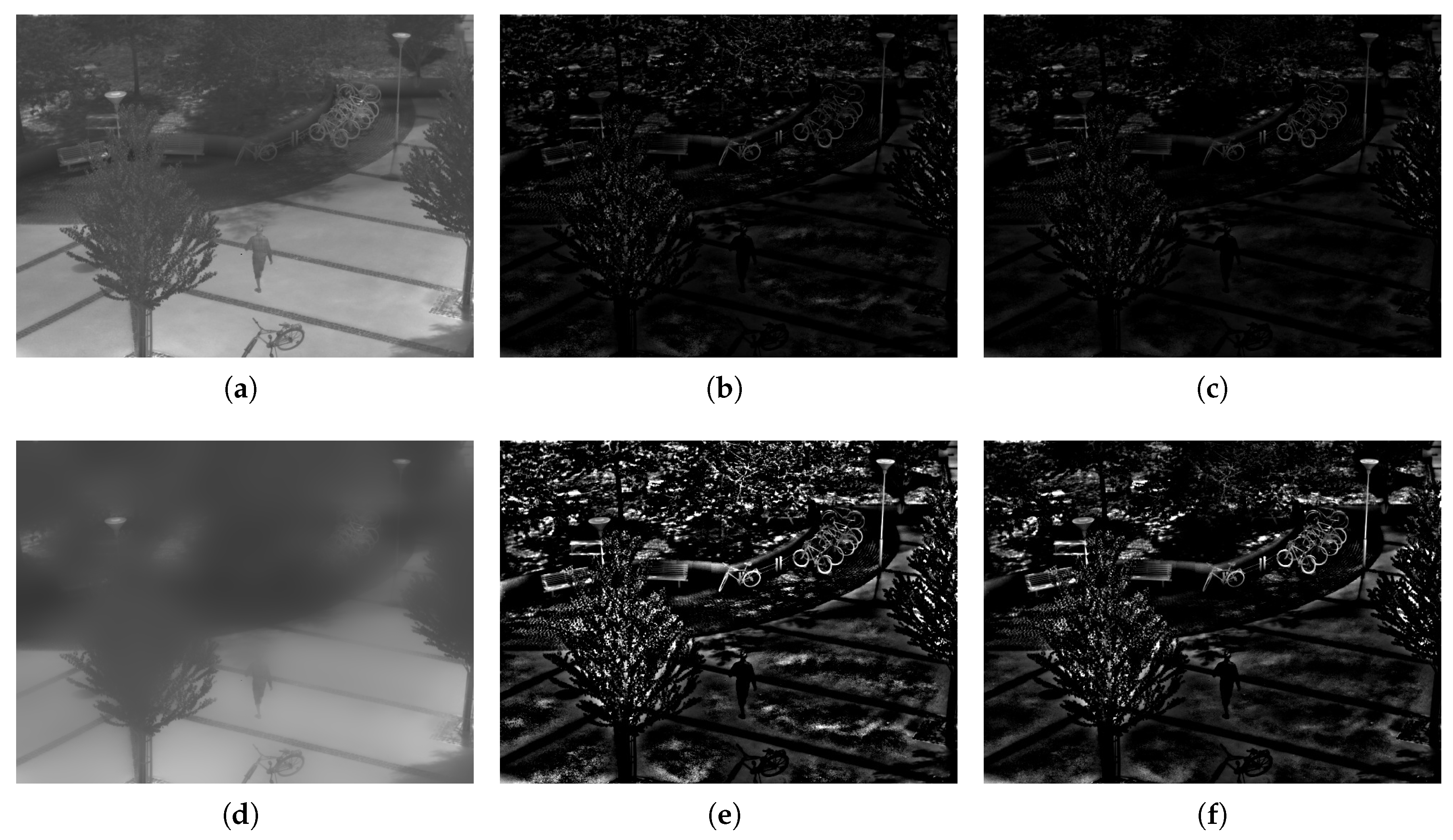
Each image can be decomposed into several layers; the details in the infrared image are typically weak. As is shown in Figure 2, the input image is one of the EOG guided transformed images, there are rich details captured by the HDR infrared sensors in the detail layers, but they are too weak to be observed.
The composition of the base layer and detail layers can be described as follows.
I e n h a n c e d = B n + α 1 D 1 + α 2 D 2 + + α n D n
The layers are linearly accumulated together, the value of each coefficient α i gives expression to the importance of the ith detail layer, the more the information in the layer, larger the α i . In order to adaptively choose the value of α i , we adopt entropy to evaluate the richness of information in each layer:
E n t r o p y ( i m ) = i = 0 1 p i log p i
where p i is the probability of gray level i in the image.
α i = C · E n t r o p y ( D i ) k = 1 n E n t r o p y ( D k ) + z i = 1 , 2 , , n
C is a fixed coefficient and z is a very small number added to prevent the denominator from being 0.
In Figure 2 the effect of the step is shown; the weak details are enhanced. The weak details in detail layers (b,c) become much clearer in (e,f). What needs to be explained is that the figures of detail layers are stretched 10 times for better visibility; the details in fact are much weaker.
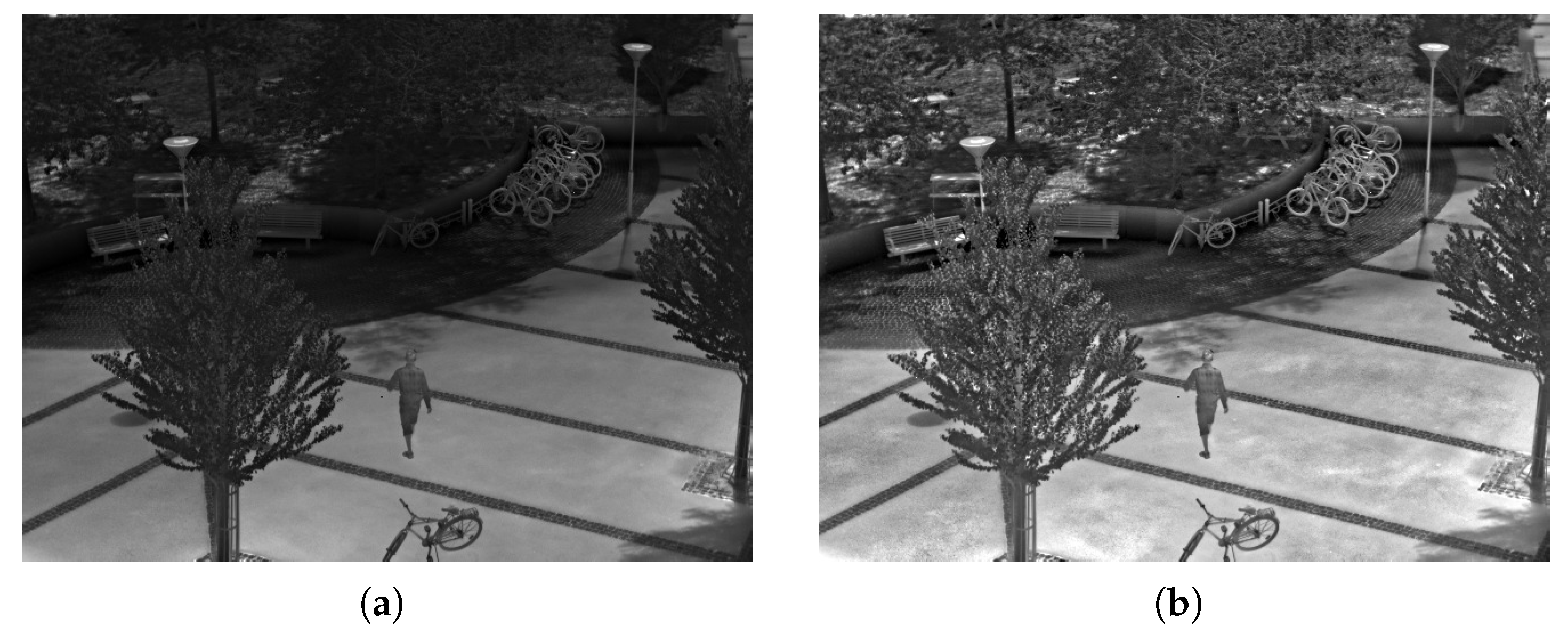
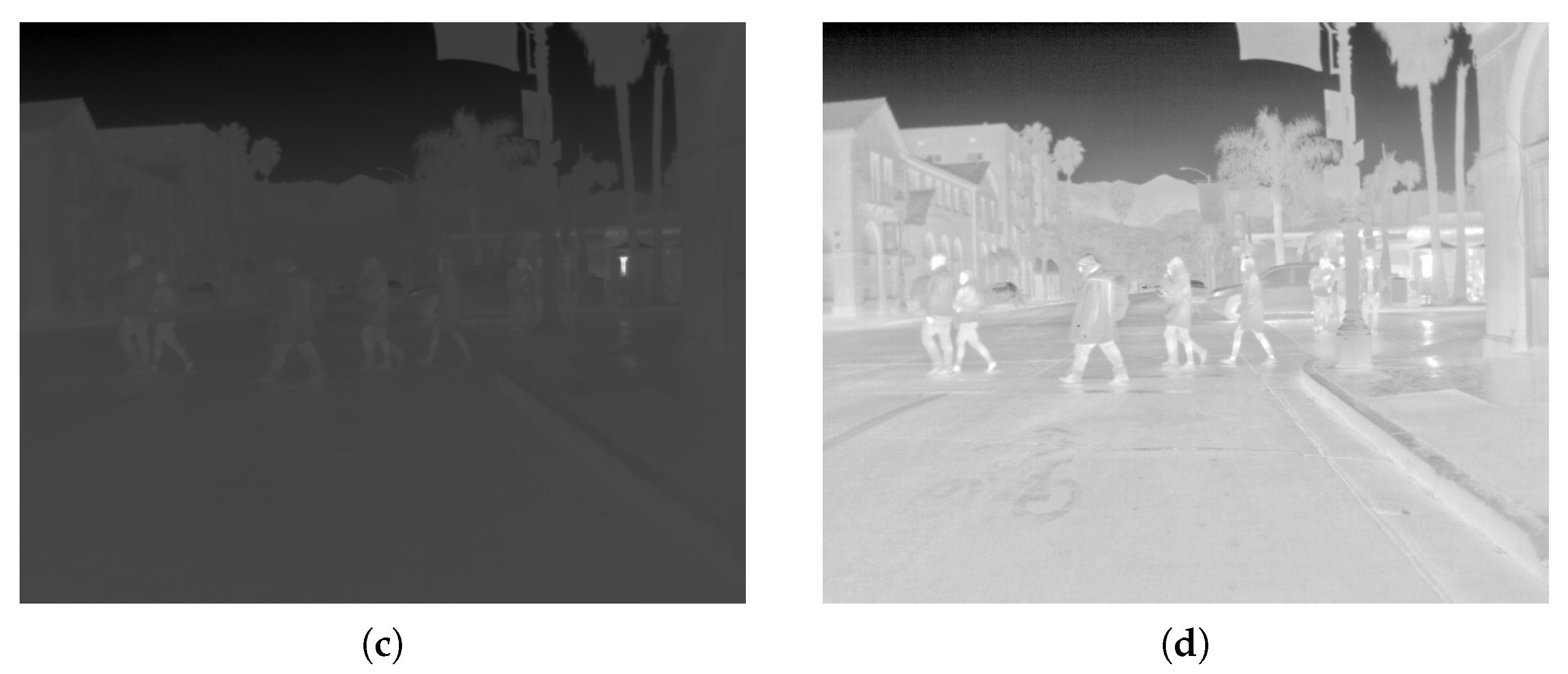
The effect of the proposed multiscale guided filter enhancement in this section can also be obviously reflected in Figure 3. There are two groups of images: panels (a,c) are results of the proposed method without the multiscale guided filter enhancement, in which the information is ambiguous, while panels (b,d) are the results of proposed method, which is much more visually comfortable.

2.3. Image Fusion

Inspired by the research hotspots including infrared and visible light images fusion and the fusion of multi-exposure images, which aim at fusing details in different images of a same scene to obtain an image with rich information, we fuse the images generated by previous steps. We adopt a method [29] with clear mathematical principles and high computational efficiency.
Through the steps above, a set of enhanced images in different brightness from the original image can be generated. We regard those images as multi-exposed images. In order to maintain local details well, we block the image in the fusion. Let { i k n } = { i k n | 1 < k < K } be a set of column vectors of N 2 dimensions expanded from the blocks at the identical location of the source images that contains K images in multi-brightness. k means the block is from the kth image of the set, n means the nth location. The elements of the vector are value of each pixel in the image block. N is the side length of the image block. n corresponds to the position of the patch in the entire image. In order to express, analyze, and process the feature of a block, the vector i k n can be decomposed into three components, including signal strength p k n . Signal structure s k n and mean intensity μ i k n . The definitions of the components are chiefly as follows.
i k n = i k n μ i k n · i k n μ i k n i k n μ i k n + μ i k n = p k n · s k n + μ i k n
μ i k n is a vector, in which all the elements equal to the mean value of i k n .
p k n = i k n μ i k n
s k n = i k n μ i k n i k n μ i k n
Obviously, the contrast of an image block can be directly reflected by the signal strength component p k n = i k n μ i k n . Generally speaking, the higher the contrast, the clearer the block or image. While the excessive contrast may trigger an unrealistic scene. Considering the input images (blocks) are undistorted, we could assume that the block has the largest contrast corresponds to the optimal visibility. Therefore, we choose the highest signal strength of all source image blocks as the signal strength of the fused image block:
p n ^ = max 1 < k < K p k n
Determine the structure of the set of image blocks as a series of unit length vectors s k n = i k n μ i k n i k n μ i k n ( 1 k K ) , and each one points to a direction in the vector space. The structure of the fused image block should represent the structures of the series of image blocks. Specifically, the relationship between the structure of fused block and the input blocks is defined in a simple but effective way:
s n ¯ = k = 1 K p k n ρ · s k n k = 1 K p k n ρ
s n ^ = s n ¯ s n ¯
The definition of mean intensity of each block is
μ n ^ = k = 1 K L ( μ k , μ i k n ) · μ i k n k = 1 K L ( μ k , μ i k n )
where L ( μ k , μ i k n ) is a weighting function which is controlled by the mean value of the kth whole image μ k and the mean value of the current block μ i k n in the kth image. L ( · ) should be relatively large when the block i k n is in a well-exposed region, and vice versa. To specify it, we adopted a two-dimensional Gaussian function:
L ( μ k , μ i k n ) = e x p [ ( μ k 0.5 ) 2 2 σ g + ( μ i k n 0.5 ) 2 2 σ l ]
When signal strength p n ^ , signal structure s n ^ , and mean intensity μ n ^ are computed, the new vector i n ^ , which means the vector of the fused image block, can be defined and the block can be reconstructed:
i n ^ = p n ^ · s n ^ + μ n ^
The blocks from the source sequence are obtained by a moving window with a fixed stride D. The pixels in the overlapping blocks are averaged to produce the final output of this step.

2.4. Outliers Filtering

Generally, there are still some outliers in the image, which are usually the brightest or darkest. Specifically, the maximum or minimum value in the image may be the outliers of the image, which affect the result of dynamic range adjustment. To cope with the problem, we have adopted a simple and effective method.
For instance, to avoid manual selection of the parameters with experience, we assume that there are two outliers in each row or in each patch with fixed size a. Take an image in size of a × b as the example. First, take every pixel value in the whole image in descending order. Then, pick out the a t h value as the minimum value f m i n and the a t h last value as the maximum value f m a x . Finally, adjust the image according to the effective values.
I o u t p u t = 255 I ^ f m i n f m a x f m i n

3. Experiment Results

3.1. Experimental Settings

In order to measure the effect and the efficiency of the proposed method.Multiple 16 bits infrared images selected from typical scenes in databases FLIR Thermal Starter Dataset Version 1.3 [31] and LTIR Dataset Version 1.0 [32] were utilized for testing. The information of the images including image size and dynamic range is listed in Table 1. Meanwhile, four well-established methods (HE [1], CLAHE [5], MSR [23], and Reinhard [24]) and two novel approaches (AHPBC [6] and LEP [14]) were introduced for comparison. In those methods, we select the parameters as the authors advised or with experience.
In Section 2.1.2 (Equation (4)), the three brightness intervals (bright S 1 , moderate S 2 , and dark S 3 ) are set as follows, S 1 = [ 0.1 , 0.7 ] , S 2 = ( 0.7 , 1.5 ] , and S 3 = ( 1.5 , 8 ] .
In Section 2.2.1 (Equation (6)), we set the value of ε be related to the variance of the entire image, because the effect of ε is determining whether it is an edge should be preserved. In our experiment, ε = σ i 3 , where σ i is the variance of the entire image.
In Section 2.2.2 (Equation (11)), the values of α k determine the enhancement of the details. Throughout our experiment, we obtain two detail layers, and in Equation (13), C = 7 and z = 0.0001 .
In Section 2.3 (Equation (18)), ρ determines the contribution of each block to the fused block’s structure. Obviously, the contribution increases along with the strength of the block. Theoretically, ρ > 0 is feasible. We set ρ = 4 in our experiment. In Equation (21), σ g and σ l control the spread of the profile along μ k and l k . We set σ g = 0.2 and σ l = 0.5 , a smaller value of σ g relative to σ l is important to generate results with good visual impression. Additionally, we set the size of blocks and the moving window stride: N = 11 and D = 2 , as the author advised.
Throughout the paper, parameters mentioned above are adopted for typical infrared images with different characteristics. Results have demonstrated that the proposed method is capable of effectively enhancing IR image.

3.2. Visual Comparisons

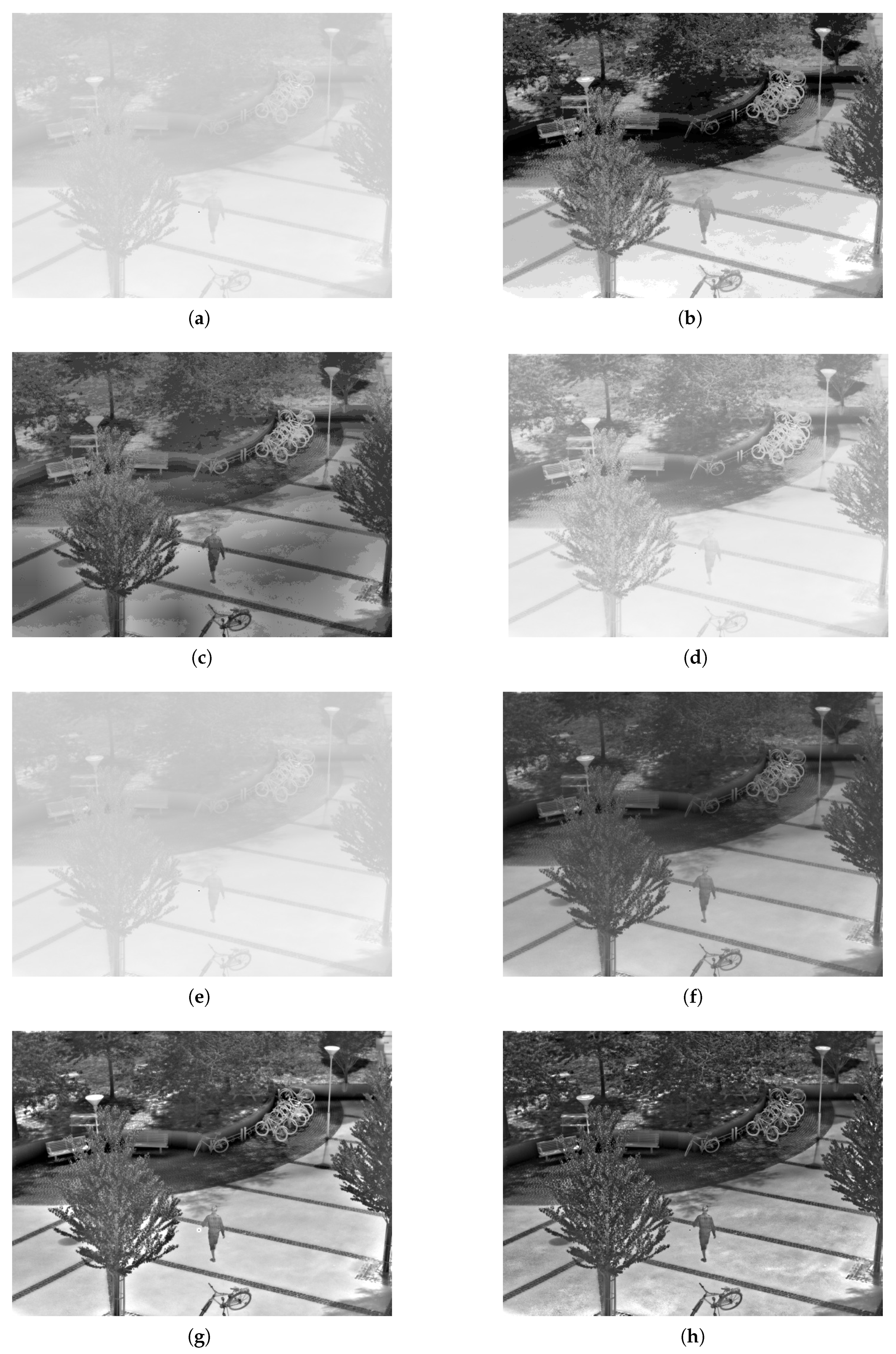
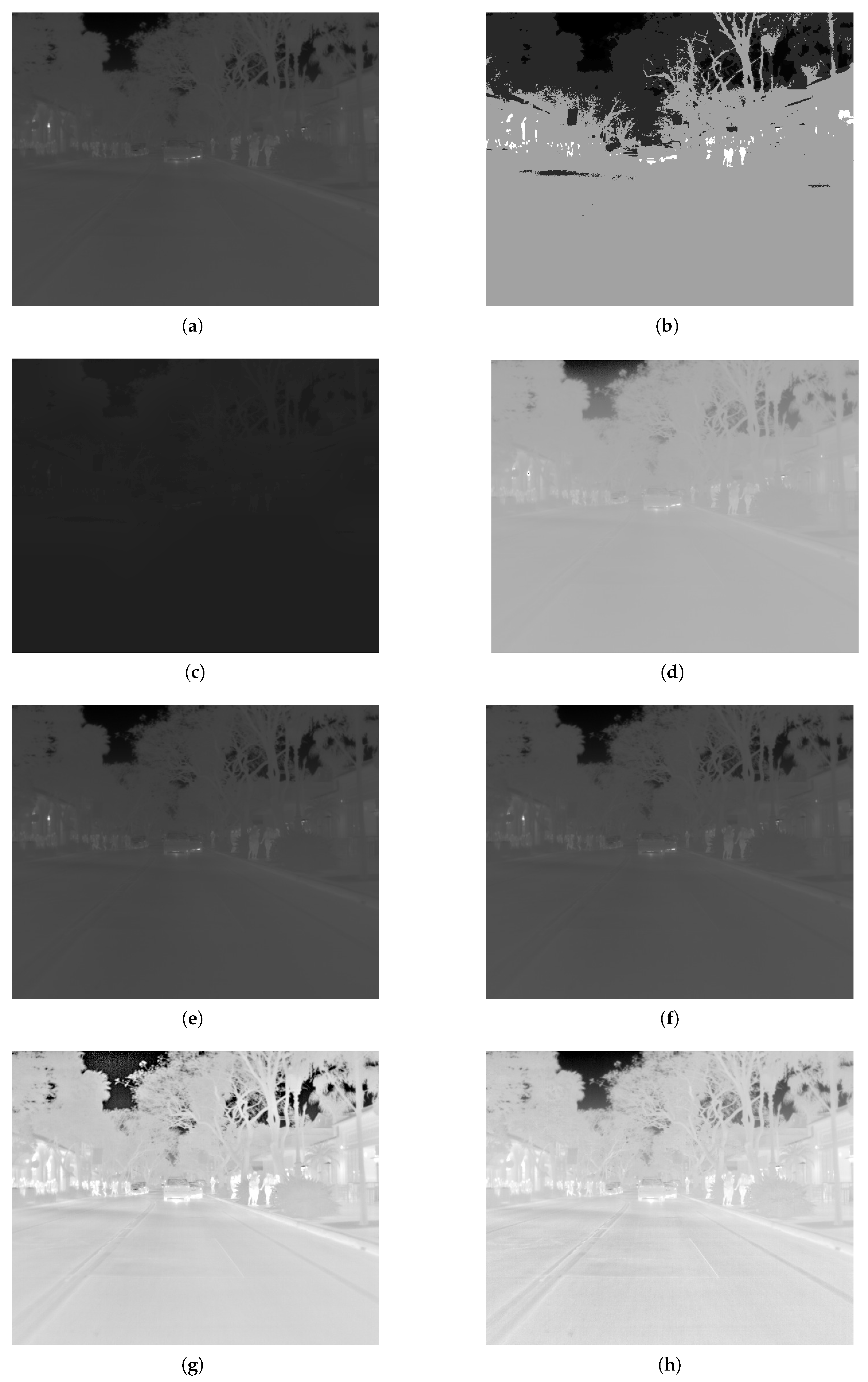
To compare the effects of the methods intuitively, the enhanced results of the algorithms are given in Figure 4, Figure 5, Figure 6, Figure 7, Figure 8, Figure 9 and Figure 10. We discuss the results in detail in Section 4.

3.3. Quantitative Comparison

Generally, good display performance means high clarity and even gray level distribution. In order to do the quantitative comparison, the Tenengrad [33], Entropy, Naturalness Image Quality Evaluator (NIQE) [34], and Perception-based Image Quality Evaluator (PIQE) [35] are introduced. They are widely used in evaluating the quality of an image.
The Tenengrad is written as
G x = 1 0 1 2 0 2 1 0 1
G y = 1 2 1 0 0 0 1 2 1
S ( x , y ) = G x I ( x , y ) + G x I ( x , y )
T e n e n g r a d = 1 n x y S ( x , y )
where I ( i , j ) denotes the gray value of the pixel ( x , y ) , * denotes convolution, and n is the number of pixels in image.
The Tenengrad is utilized to reflect the clarity of the whole image. Theoretically, the larger the Tenengrad value is, the higher the contrast, and the better the visibility of the details of the image. The calculation Tenengrad results are listed in Table 2.
The even distribution of the pixel values of the image is another goal of image enhancement. And the entropy of an image is a common approach to reflect the pixel value’s distribution. Specifically and theoretically, the larger the entropy value is, the more evenly the gray levels distributed. The entropy of an 8 bit image is written as
E n t r o p y ( i m ) = i = 0 255 p i log p i
where p i is the probability of gray level i in the image. The calculation Entropy results are listed in Table 3.
NIQE measures the distance between the NSS-based features calculated from image to the features obtained from an image database used to train the model. The features are modeled as multidimensional Gaussian distributions. We calculate it by the Matlab function n i q e ( ) , which returns a non-negative scalar. Theoretically, the lower value of NIQE is, the better the perceptual quality of the image. The results are listed in Table 4.
PIQE calculates the no-reference quality score for an image through block-wise distortion estimation. We calculate it by the Matlab function p i q e ( ) , which returns a non-negative scalar in the range [0, 100]. The PIQE score is inversely correlated to the perceptual quality of an image. A low PIQE value indicates high perceptual quality and high PIQE value indicates low perceptual quality. The results are listed in Table 5.

3.4. Running Time Comparison

In order to do an efficiency comparison, the above-listed algorithms are tested, using MATLAB R2018b on a personal computer (Intel core i5-8250U; CPU:1.60 GHz; Memory: 8 GB). The size of the tested images are listed in Table 1. The calculation time results are listed in Table 6.

4. Discussion

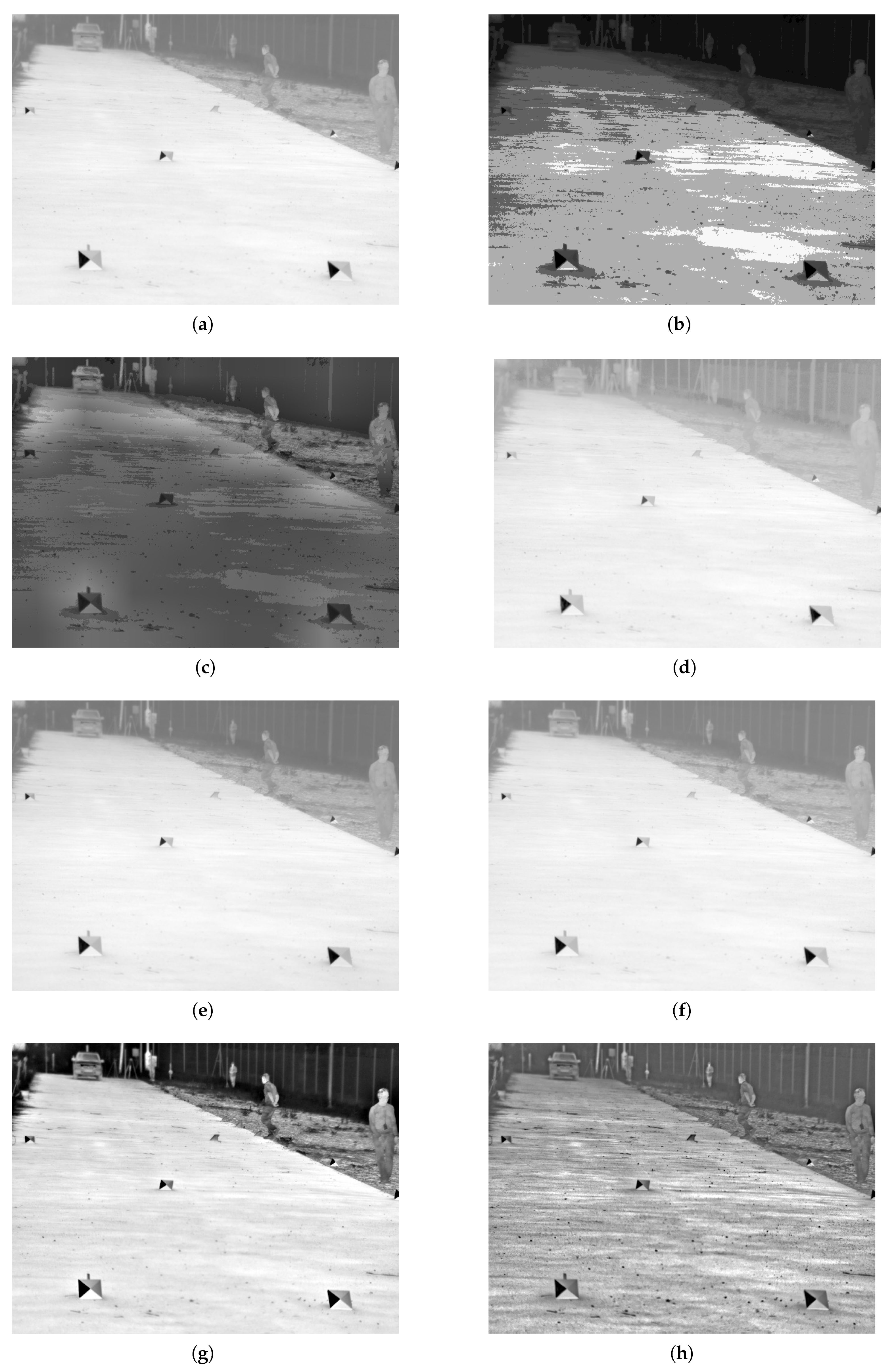
Image group Figure 4 is an example of infrared images of rich scene information including human, bicycles, benches, ground, and so on. HE and CLAHE enhanced the contrast, while a large amount of local details lost. The AHPBC and MSR can enhance the details to some extent, while the dynamic range of the result image is so small that the visibility is poor. The result of Reinhard is visually comfortable but the some texture information is still ambiguous. LEP can enhance the image well in general, but generates a halo. Compared with other six approaches, our method meets the best performance.
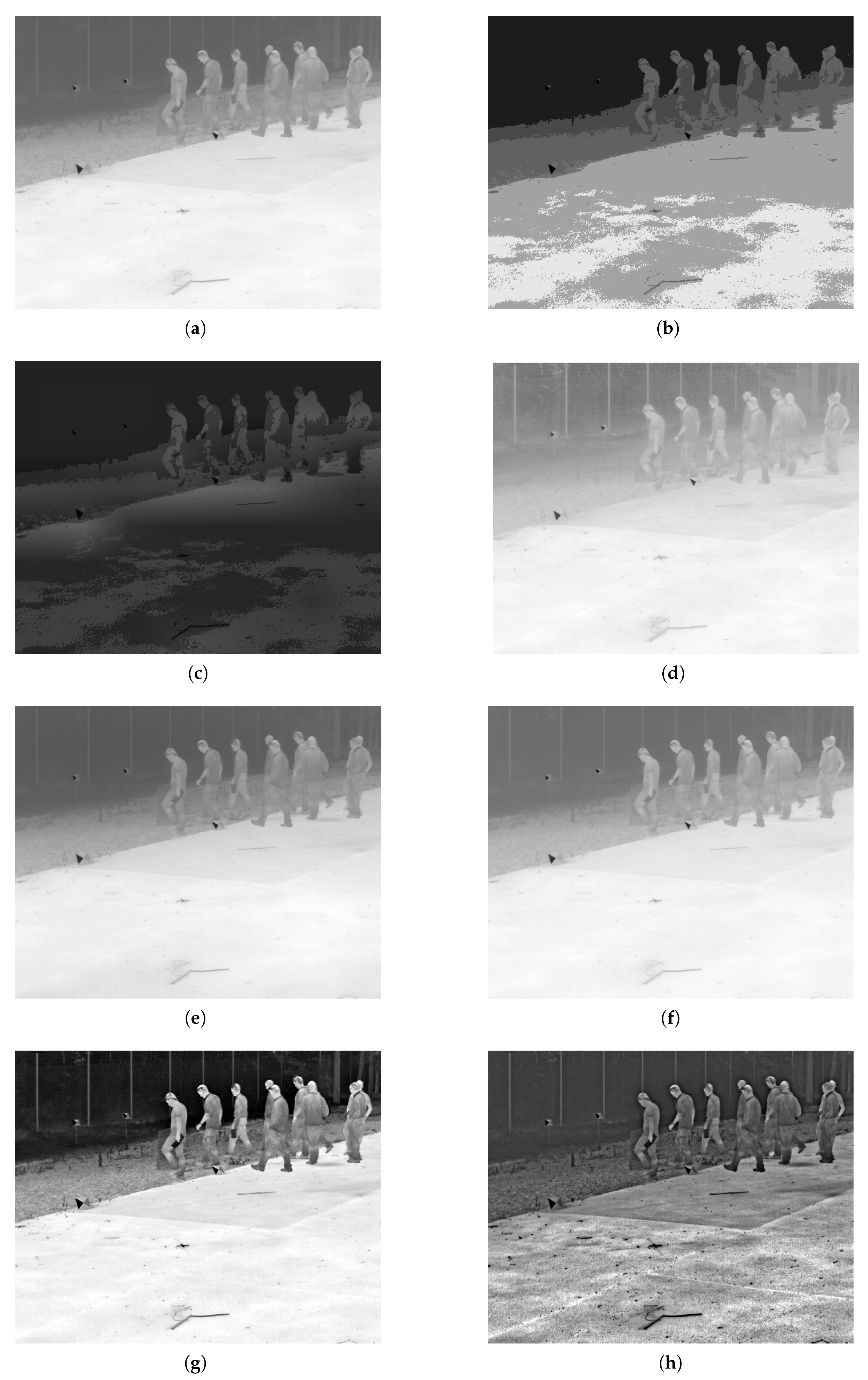
Image group Figure 5 and Figure 6 are examples of low contrast image, which contains many details about the texture. The dynamic range of the original IR image is so narrow that HE and CLAHE fail in the enhancement of the details, while some regions in their results are over-enhanced, and some noises are generated. AHPBC, MSR, and Reinhard can preserve the global contrast but has a relatively weak compatibility in the enhancement of the local details. LEP can successfully enhance the edge of the humans in the image, but some tiny details like the texture of the road are still dim. Our method yields the best enhancement results, producing global detail enhancement without noise generation.
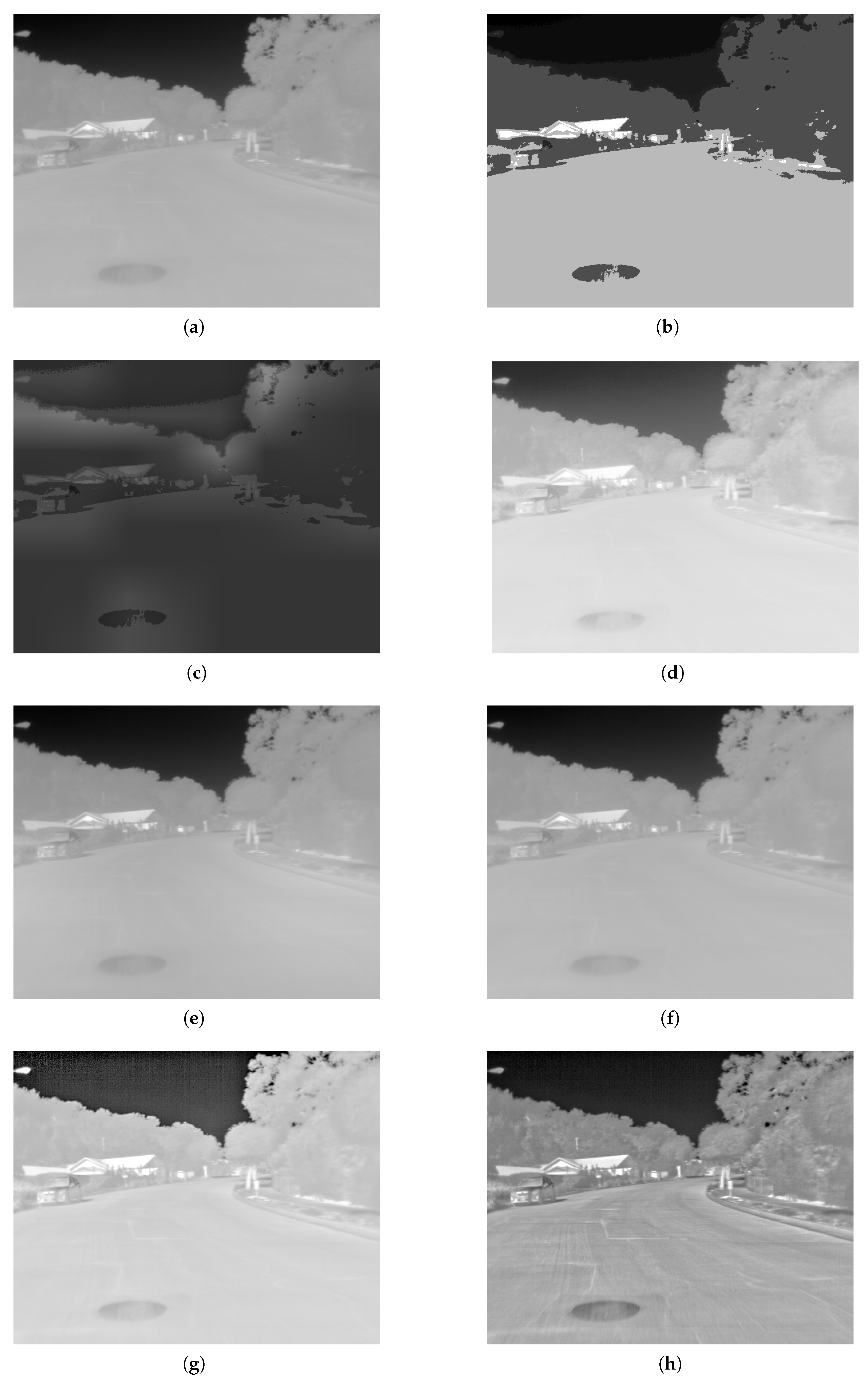
Image group Figure 7 and Figure 8 are examples of foggy images. Details like outlines of trees and human are unobservable in the results of HE and CLAHE, and the backgrounds are distorted. Compared with the original linear mapped image, the results of AHPBC and Reinhard are still blurred, even though there might be a great change in brightness. MSR can increase the contrast to some extent, but the effect on local detail enhancement is relatively weak. The noise in the result of LEP is obvious. It can be indicated by the comparison of the results in Figure 7 and Figure 8 that the proposed method creates the most visually comfortable results, which reveal the details most fully.
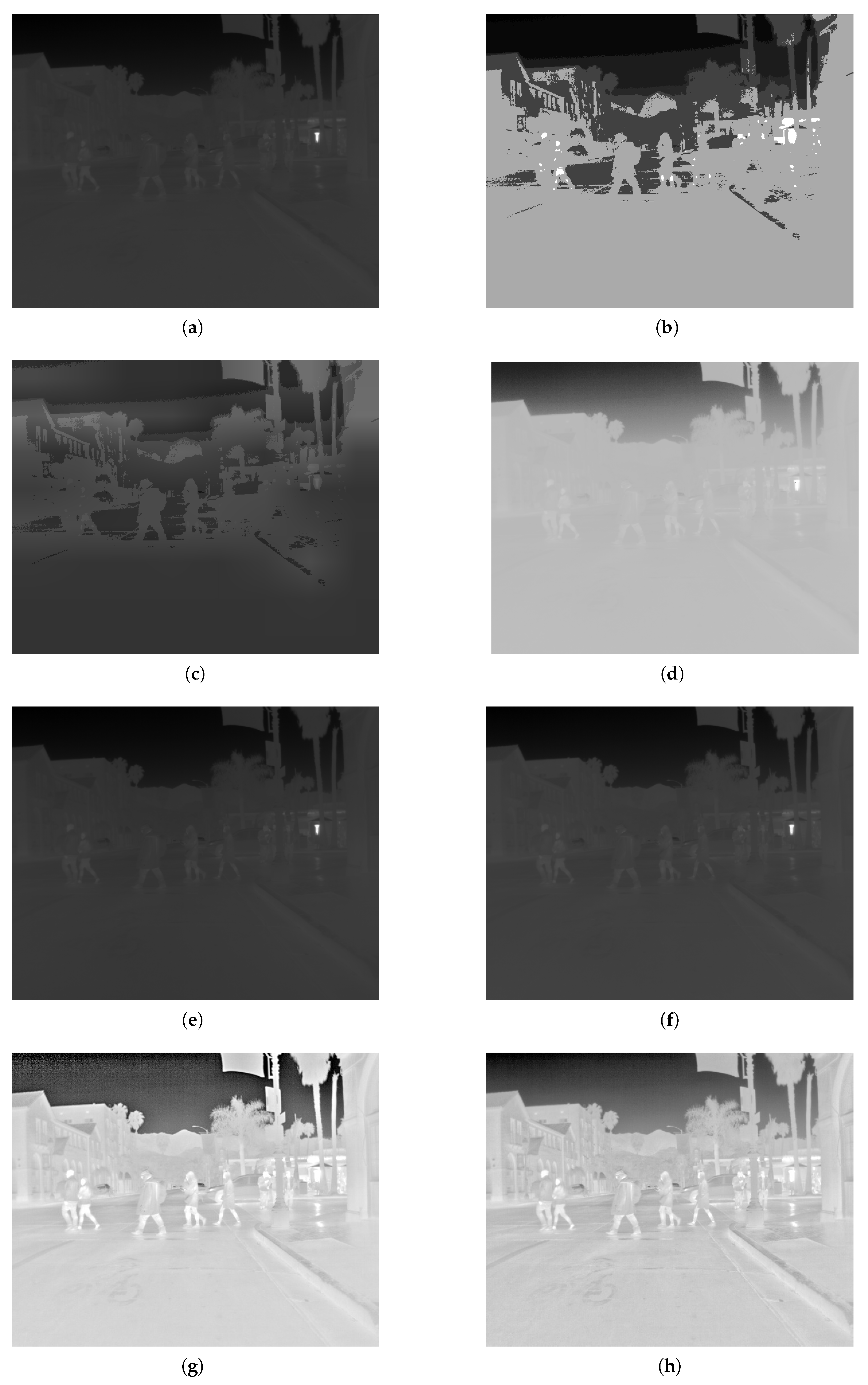
Image group Figure 9 and Figure 10 are examples of image with blurred details. Due to low contrast and weak details in the original image, HE and CLAHE not only fail to reproduce the details, but also generate noises. Objects such as trees, buildings, and pedestrians in AHPBC’s results are blurred. The results of MSR and Reinhard are too dark to observe the information. Relatively, the results of LEP and the proposed method are visually pleasing; comparing with the results of LEP, noise in the proposed results is weaker.
The results of the Tenengrad for the test images are shown in the Table 2. In theory, the higher value of Tenengrad, the clearer the entire image. In accordance with the result of visual comparisons, the proposed method and LEP achieve higher Tenengrads.
As being reported in Table 3, comparing about the entropy, the proposed method and LEP have the robust result, and our method obtains the slightly better value than LEP does. Practically, there are more details in the results of our proposed method.
As being reported in Table 4, comparing about the NIQE, lower value of NIQE reflect better perceptual quality of image. the overall difference of AHPBC, MSR, Reinhard, LEP, and our proposed method is not obvious.
As being reported in Table 5, lower value of NIQE reflect better perceptual quality of image. In general, the proposed method and LEP achieve better results, but the average result of our proposed method is the best.
As being reported in Table 6, as our approach introduce multiscale analysis and image fusion, the calculation time of the proposed algorithm is much more than the conventional and famous methods HE, CLAHE, MSR, and Reinhard. Our method runs relatively slower than LEP, but more quickly than AHPBC. How to accelerate our algorithm is one of the key points of our future work. Hardware acceleration is one of our choices. After optimization, our method is very likely to process image on real-time application.
All in all, performance of the proposed algorithm is verified by experiments with images with various characteristics. The above analysis of the results shows that the proposed method has strength in detail enhancement of the HDR infrared image. The dynamic range compression and detail enhancement results are visually comfortable without excessively obvious noise.

5. Conclusions

In this paper, a novel high dynamic range infrared image enhancement method is introduced. This method is capable of compressing the dynamic range, adjusting the gray levels, and enhancing the details effectively. The proposed approach is mainly based on adaptive Gamma correction, multiscale guided filter, and image fusion. First, in order to keep the weak global details in different area, we adopt an EOG-guided Gamma transformation, which is adaptive to adjust the original normalized image into multiple brightness levels. Second, the multiscale guided filter is utilized iteratively to decompose each brightness image into a base layer and several detail layers. Details in each image are enhanced separately and composed adaptively. Third, to obtain the image with global details of the input image, enhanced image in each brightness is fused together. Last, we filter out the bad pixels and adjust the dynamic range before outputting the image. Tested on HDR IR images of different scenes with sundry details and background, the experiment result indicates that the proposed method can compress the dynamic range while higher the contrast, enhance the details effectively, and generate a visually pleasing result. It should be pointed out that in the step of guided transformation, the EOG function is just chosen to guarantee the simplicity and correctness of the algorithm. That is to say, the function could be changed according to the case with flexibility in the future work. Meanwhile, the method of the enhancement of the decomposed layers could also be extended, which also provides new point for the research.

Author Contributions

F.C. proposed the original idea, performed the experiment and wrote the original manuscript; J.Z. contributed to the direction, content, and revised the manuscript and funding acquisition; project administration J.C.; T.X. revised the manuscript; G.L. contributed to the content; and X.P. contributed to the content, revised the manuscript and project administration. All authors have read and agreed to the published version of the manuscript.

Funding

We are grateful to the financial support of the National High Technology Research and Development Program of China (863 Program), grant number G158207.

Conflicts of Interest

The authors declare no conflict of interest.

References

  1. Sanchez-Reillo, R.; Tamer, S.; Lu, G.; Duta, N.; Keck, M. Histogram Equalization; Springer: New York, NY, USA, 2009. [Google Scholar]
  2. Song, Y.F.; Shao, X.P.; Xu, J. New enhancement algorithm for infrared image based on double plateaus histogram. Infrared Laser Eng. 2008, 2, 308–311. [Google Scholar]
  3. Vickers, V.E. Plateau equalization algorithm for real-time display of high-quality infrared imagery. Opt. Eng. 1996, 35, 1921. [Google Scholar] [CrossRef]
  4. Wang, B.J. A real-time contrast enhancement algorithm for infrared images based on plateau histogram. Acta Photonica Sin. 2006, 48, 77–82. [Google Scholar] [CrossRef]
  5. Zuiderveld, K. Contrast Limited Adaptive Histogram Equalization. In Graphics Gems; Academic Press Professional, Inc.: San Diego, CA, USA, 1994; pp. 474–485. [Google Scholar]
  6. Wan, M.; Gu, G.; Qian, W.; Ren, K.; Chen, Q.; Maldague, X. Infrared Image Enhancement Using Adaptive Histogram Partition and Brightness Correction. Remote Sens. 2018, 10, 682. [Google Scholar] [CrossRef] [Green Version]
  7. Liang, K.; Yong, M.; Yue, X.; Bo, Z.; Rui, W. A new adaptive contrast enhancement algorithm for infrared images based on double plateaus histogram equalization. Infrared Phys. Technol. 2012, 55, 309–315. [Google Scholar] [CrossRef]
  8. Kim, J.Y.; Kim, L.S.; Hwang, S.H. An advanced contrast enhancement using partially overlapped sub-block histogram equalization. IEEE Trans. Circuits Syst. Video Technol. 2001, 11, 475–484. [Google Scholar]
  9. Fattal, R.; Lischinski, D.; Werman, M. Gradient Domain High Dynamic Range Compression. ACM Trans. Graph. 2002, 21. [Google Scholar] [CrossRef] [Green Version]
  10. Zhang, F.; Xie, W.; Ma, G.; Qin, Q. High dynamic range compression and detail enhancement of infrared images in the gradient domain. Infrared Phys. Technol. 2014, 67, 441–454. [Google Scholar] [CrossRef]
  11. Durand, F.; Dorsey, J. Fast bilateral filtering for the display of high-dynamic-range images. ACM Trans. Graph. 2002, 21, 257–266. [Google Scholar] [CrossRef] [Green Version]
  12. He, K.; Sun, J.; Tang, X. Guided Image Filtering. IEEE Trans. Pattern Anal. Mach. Intell. 2013, 35, 1397–1409. [Google Scholar] [CrossRef]
  13. Li, S.; Kang, X.; Hu, J. Image Fusion With Guided Filtering. IEEE Trans. Image Process. 2013, 22, 2864–2875. [Google Scholar] [PubMed]
  14. Gu, B.; Li, W.; Zhu, M.; Wang, M. Local Edge-Preserving Multiscale Decomposition for High Dynamic Range Image Tone Mapping. IEEE Trans. Image Process. 2013, 22, 70–79. [Google Scholar]
  15. Bai, X.; Zhou, F.; Xue, B. Image enhancement using multi scale image features extracted by top-hat transform. Opt. Laser Technol. 2011, 44, 328–336. [Google Scholar] [CrossRef]
  16. Bai, X.; Zhou, F.; Xue, B. Infrared image enhancement through contrast enhancement by using multiscale new top-hat transform. Infrared Phys. Technol. 2011, 54, 61–69. [Google Scholar] [CrossRef]
  17. Zhan, B.; Wu, Y. Infrared Image Enhancement Based on Wavelet Transformation and Retinex. In Proceedings of the 2010 Second International Conference on Intelligent Human-machine Systems & Cybernetics, Nanjing, China, 26–28 August 2010. [Google Scholar]
  18. Mccann, J.J. Lightness and retinex theory. J. Opt. Soc. Am. 1970, 61, 1–11. [Google Scholar]
  19. Land, E.H. The Retinex Theory of Color Vision. Sci. Am. 1977, 237, 108–129. [Google Scholar] [CrossRef] [PubMed]
  20. Rahman, Z.U.; Jobson, D.J.; Woodell, G.A. Retinex processing for automatic image enhancement. J. Electron. Imaging 2004, 13, 100–110. [Google Scholar]
  21. Pu, Y.F.; Zhang, N.; Wang, Z.N.; Wang, J.; Yi, Z.; Wang, Y.; Zhou, J.L. Fractional-Order Retinex for Adaptive Contrast Enhancement of Under-Exposed Traffic Images. IEEE Intell. Transp. Syst. Mag. 2019. [Google Scholar] [CrossRef]
  22. Jobson, D.; Rahman, Z. Properties and performance of a center/surround retinex. IEEE Trans. Image Process. 1997, 6, 451–462. [Google Scholar] [CrossRef]
  23. Rahman, Z.; Jobson, D.J.; Woodell, G.A. Multi-scale retinex for color image enhancement. In Proceedings of the 3rd IEEE International Conference on Image Processing, Lausanne, Switzerland, 19 September 2002. [Google Scholar]
  24. Reinhard, E.; Stark, M.; Shirley, P.; Ferwerda, J. Photographic tone reproduction for digital images. ACM Trans. Graph. 2002, 21, 267–276. [Google Scholar] [CrossRef] [Green Version]
  25. Reinhard, E.; Pouli, T.; Kunkel, T.; Long, B.; Ballestad, A.; Damberg, G. Calibrated image appearance reproduction. ACM Trans. Graph. 2012, 31, 1–11. [Google Scholar] [CrossRef]
  26. Abebe, M.A.; Pouli, T.; Larabi, M.C.; Reinhard, E. Perceptual Lightness Modeling for High Dynamic Range Imaging. ACM Trans. Appl. Percept. 2017, 15, 1. [Google Scholar] [CrossRef]
  27. Ma, J.; Zhou, Z.; Wang, B.; Zong, H. Infrared and visible image fusion based on visual saliency map and weighted least square optimization. Infrared Phys. Technol. 2017, 82, 8–17. [Google Scholar] [CrossRef]
  28. Saeedi, J.; Faez, K. Infrared and visible image fusion using fuzzy logic and population-based optimization. Appl. Soft Comput. 2012, 12, 1041–1054. [Google Scholar] [CrossRef]
  29. Ma, K.; Zhou, W. Multi-exposure image fusion: A patch-wise approach. In Proceedings of the 2015 IEEE International Conference on Image Processing, Quebec City, QC, Canada, 27–30 September 2015. [Google Scholar]
  30. Ma, K.; Li, H.; Yong, H.; Wang, Z.; Meng, D.; Zhang, L. Robust Multi-Exposure Image Fusion: A Structural Patch Decomposition Approach. IEEE Trans. Image Process. 2017, 26, 2519–2532. [Google Scholar] [CrossRef] [PubMed]
  31. FLIR Thermal Starter Dataset Version 1.3. Available online: https://www.flir.com/oem/adas/adas-dataset-form/ (accessed on 16 August 2019).
  32. Berg, A.; Ahlberg, J.; Felsberg, M. A Thermal Object Tracking Benchmark. In Proceedings of the 2015 12th IEEE International Conference on Advanced Video and Signal Based Surveillance (AVSS), Karlsruhe, Germany, 25–28 August 2015. [Google Scholar]
  33. Tenenbaum, J.M. Accommodation in Computer Vision; Computer Science Department, Stanford University: Stanford, CA, USA, 1971. [Google Scholar]
  34. Mittal, A.; Soundararajan, R.; Bovik, A.C. Making a “completely blind” image quality analyzer. IEEE Signal Process. Lett. 2012, 20, 209–212. [Google Scholar] [CrossRef]
  35. Venkatanath, N.; Praneeth, D.; Bh, M.C.; Channappayya, S.S.; Medasani, S.S. Blind image quality evaluation using perception based features. In Proceedings of the 2015 Twenty First National Conference on Communications (NCC), Mumbai, India, 27 February–1 March 2015; pp. 1–6. [Google Scholar]
Figure 1. The proposed framework.
Applsci 10 06262 g001
Figure 2. (a) Input Image. (b) Detail Layer 1. (c) Detail Layer 2. (d) Base Layer. (e) Enhanced Detail Layer 1. (f) Enhanced Detail Layer 1.
Applsci 10 06262 g002
Figure 3. (a) Result 1 without multiscale guided filter enhancement. (b) Result 1 with multiscale guided filter enhancement. (c) Result 2 without multiscale guided filter enhancement. (d) Result 2 with multiscale guided filter enhancement.
Applsci 10 06262 g003aApplsci 10 06262 g003b
Figure 4. Comparison results 1 (Image of Complex Scene). (a) Linear Mapping. (b) histogram equalization (HE). (c) contrast-limited adaptive histogram equalization (CLAHE). (d) AHPBC. (e) MSR. (f) Reinhard. (g) LEP. (h) Proposed result.
Applsci 10 06262 g004
Figure 5. Comparison Results 2 (Low Contrast Image). (a) Linear Mapping. (b) HE. (c) CLAHE. (d) AHPBC. (e) MSR. (f) Reinhard. (g) LEP. (h) Proposed result.
Applsci 10 06262 g005
Figure 6. Comparison Results 3 (Low Contrast Image). (a) Linear Mapping. (b) HE. (c) CLAHE. (d) AHPBC. (e) MSR. (f) Reinhard. (g) LEP. (h) Proposed result.
Applsci 10 06262 g006
Figure 7. Comparison Results 4 (Foggy Image). (a) Linear Mapping. (b) HE. (c) CLAHE. (d) AHPBC. (e) MSR. (f) Reinhard. (g) LEP. (h) Proposed result.
Applsci 10 06262 g007
Figure 8. Comparison Results 5 (Foggy Image). (a) Linear Mapping. (b) HE. (c) CLAHE. (d) AHPBC. (e) MSR. (f) Reinhard. (g) LEP. (h) Proposed result.
Applsci 10 06262 g008
Figure 9. Comparison Results 6 (Image with Blurred Details). (a) Linear Mapping. (b) HE. (c) CLAHE. (d) AHPBC. (e) MSR. (f) Reinhard. (g) LEP. (h) Proposed result.
Applsci 10 06262 g009
Figure 10. Comparison Results 7 (Image with Blurred Details). (a) Linear Mapping. (b) HE. (c) CLAHE. (d) AHPBC. (e) MSR. (f) Reinhard. (g) LEP. (h) Proposed result.
Applsci 10 06262 g010
Table 1. Basic information of the test images.
ImageSizeMin (Gray Value)Max (Gray Value)% of the Total Gray Levels
IM1480*64001696125.880
IM2480*6409893163399.835
IM3512*640141135753.302
IM4512*640568381883.822
IM5512*640643386533.387
IM6512*6405984113228.145
IM7512*6406010100006.088
Table 2. The Tenengrad’s value of the images.
ImageLinear MappingHECLAHEAHPBCMSRReinhardLEPProposed
IM14.256218.808715.712310.59954.213711.109121.538522.3971
IM24.940312.38007.44904.77704.84714.760111.129918.1054
IM34.44598.93824.28564.73904.18214.244811.085518.5358
IM43.11444.41152.08743.62313.13463.12055.99777.8913
IM54.61915.14333.96764.64684.40704.60409.531414.9446
IM61.42277.88632.96392.75261.41581.60088.47476.7918
IM72.07788.79892.91212.91682.07382.24118.93276.8261
Table 3. The entropy of the images.
ImageLinear MappingHECLAHEAHPBCMSRReinhardLEPProposed
IM15.57353.45537.02385.35115.45627.32067.61187.5752
IM25.76552.55426.50895.68056.03525.65256.76367.1654
IM36.37332.23745.16766.19616.69406.22907.05877.4246
IM45.92891.77275.14015.71686.43125.90525.85556.6476
IM57.50172.88095.86237.49277.45407.51187.46147.8229
IM64.51741.57715.29514.37804.72774.67656.18916.3499
IM74.55041.18254.58594.55564.72234.64505.80295.8444
Table 4. The Naturalness Image Quality Evaluator (NIQE) values of the images.
ImageLinear MappingHECLAHEAHPBCMSRReinhardLEPProposed
IM12.40307.60344.75572.31482.37132.16732.56252.8865
IM23.16178.77445.80553.33523.21843.20783.48164.0588
IM33.335911.53567.49723.86023.33823.29563.97614.3825
IM47.514011.93667.51404.28404.85514.72134.21824.8106
IM53.571915.06187.28633.49613.69313.62393.63693.4917
IM64.958113.32837.42484.90654.88224.55613.93354.0222
IM73.977311.74037.96853.71863.97943.87343.58093.5237
Table 5. The Perception-based Image Quality Evaluator (PIQE) values of the images.
ImageLinear MappingHECLAHEAHPBCMSRReinhardLEPProposed
IM133.701765.397059.933533.4366533.335421.288522.890124.9244
IM230.808676.730374.356732.435032.817234.547220.324122.4031
IM316.043182.788379.374616.584219.205118.481013.866930.9339
IM474.825881.647174.825835.722437.266339.046136.491516.0016
IM552.984882.522080.267152.787654.407549.002449.437743.2992
IM665.928481.132177.741262.935664.938758.832520.687016.2914
IM758.005279.802274.038756.852352.665454.869716.859016.2839
Table 6. Running time of the test images. Unit: second.
ImageHECLAHEAHPBCMSRReinhardLEPProposed
IM10.11400.199927.77910.92250.02570.84822.5096
IM20.11950.143926.82930.17700.02841.09432.4500
IM30.11110.145530.87190.10700.21981.15432.6872
IM40.11580.138730.64250.10400.02021.13252.7946
IM50.12530.142240.46240.09900.02071.03142.6288
IM60.11120.143428.53090.09810.02081.28402.5608
IM70.14630.186927.44650.99370.02032.12502.7588