Abstract
The locomotive ability of a water strider that generates an ellipse-like spatial stroke trajectory when moving is proved to improve its moving efficiency and is seldom imitated by water strider robots. A hydrodynamic analysis can predict the performance of the robots, but research in this area is not enough. A buoyancy-supported water strider robot with the ability of producing an ellipse-like spatial stroke trajectory was designed and analyzed in this study. A semiempirical hydrodynamic model suitable for the buoyancy-supported robot was proposed to study the hydrodynamic characteristics, based on the Newton’s second law of motion. The speed, power and efficiency of the robot were analyzed on the basis of the model which confirmed that the robot performing an ellipse-like spatial stroke trajectory was conducive to its moving efficiency. The experimental results verified that the stroke mechanism produced an ellipse-like spatial trajectory in a practical application and that the robot had good mobility. The proposed hydrodynamic model was validated by comparing the theoretical speed of the robot to the experimental results.
1. Introduction
With the development of robot technology and biology, bionic robot technology has achieved considerable progress and many kinds of bionic robots have appeared over the past several decades [1,2,3,4,5]. A water strider is a small aquatic insect which can stand, glide, and leap on the surface of water. It is mainly comprised of a torso, four supporting legs, and two stroke legs. The legs of the water strider have a hairy hydrophobic structure which can let itself stand and move on the water surface with water tension. The supporting leg receives an upward supporting force on the water surface and the stroke leg is subjected to a forward drag force and an upward lift force [6,7]. The water strider has many advantages such as highly efficient locomotion, a good stability, quiet movement, and little disturbance to the water surface [8,9]. Owing to the unique advantage the water strider has of walking on the water surface and the potential applications of bionic robots inspired by water striders in many areas such as water quality monitoring, aquatic search, and rescue [10], tremendous efforts have been devoted to the development of water strider robots in recent years [9,10,11,12,13,14,15,16,17,18,19,20].
Considering that it is relative easy to implement, most of the water strider robots developed imitate the slide movement of the water strider. The first type of water strider robots were designed based on the water surface tension support [9,10,13,14,15,16]. The studies on these robots primarily focused on the selection of the proper hydrophobic materials for the stroke legs and supporting legs to imitate the hydrophobic properties of the water strider. However, due to the low water surface tension, the load capacity of such bionic robots is generally very limited, which in turn greatly restricts their application. Therefore, water strider robots with a much stronger load capacity (e.g., buoyancy-supported water strider robots) have also begun to be considered [17,18,19,20]. This type of the robots uses floats as the support legs and paddles as the stroke legs, which improve the load capacity and practicability of these robots. This article adopts the latter scheme to develop the water strider robot.
The current studies on water strider robots mainly concentrate on structural design and movement analysis. However, the robotic counterpart that can generate an ellipse-like spatial stroke trajectory, just as the real water strider does, when moving on the water surface is very limited. The ellipse-like spatial stroke trajectory produced by the water strider via adjusting its joints when rowing with its stroke legs [10,21] facilitates a larger stroke length for the stroke leg and effectively helps to improve the working efficiency. Yan et al. [10] designed a special actuating leg using a cam-link mechanism which could generate an ellipse-like spatial trajectory similar to that of a real water strider. Due to the limited water surface tension between the supporting legs and the water surface, the load capacity and propulsion provided by the cam-link mechanism were very limited. Song and Sitti [9] superimposed two 1D actuators to create an elliptical path of the actuating leg. The actuating leg was driven by the piezoelectric actuators which is difficult to accurately control and the propulsion generated was small. At present, there is no buoyancy-supported water strider robot capable of an ellipse-like spatial stroke trajectory.
The hydrodynamics are important to ascertain the propulsion, resistance, and evaluate the efficiency of the robots. It is also helpful to confirm the speed of the robots. For the hydrodynamic studies on the water strider robots based on the water surface tension support, Suhr et al. [14] determined the supporting force of a water strider robot by accumulating the surface tension force and buoyancy of the supporting legs. Song and Sitti [9] analyzed the force of the water strider robot more completely and calculated the moving speed of the robot based on the work conducted by Bush et al. [22]. Since the water strider robot to be developed in this paper is a buoyancy-supported robot similar to a ship or an autonomous underwater vehicle (AUV), the above methods to calculate the hydrodynamics of the robots are not suitable for our study. For hydrodynamic studies on the buoyancy-supported water strider robots are few. Some studies on the hydrodynamics of similar water surface robots were based on a formula which calculates the drag force of the external flow past an object [23,24]. They used this formula to calculate the propulsion of the robots by considering the dimensionless coefficient in the formula as a constant. Since the contact situation between the stroke leg of the water strider robot with the water varies greatly over time and the dimensionless force coefficient is variable, this method cannot directly apply to the propulsion calculation of the water strider robot.
In our previous research, which is a shorter conference version of this paper, a buoyancy-supported water strider robot was developed that could imitate the water strider to form an ellipse-like spatial stroke trajectory [25]. Its stroke mechanism is a linear guide and rotation coupled mechanism and does not generate vertical force which is conducive to the motion stability of the robot. However, the hydrodynamic characteristic of the robot has not been introduced and the effectiveness of the ellipse-like spatial stroke trajectory on the robot motion has not been analyzed. In this paper, a semiempirical hydrodynamic mode for the buoyancy-supported water strider robot is established by Newton’s second law of motion. The hydrodynamic mode used the differential method to enable the formula, calculating the drag force of the external flow past an object, to calculate the propulsion of the paddle which rotates over time. The coefficient in the hydrodynamic mode was measured by a quasi-static approach and fitted with a quadratic polynomial function to get a continuous relationship with the rotational angle of the paddle. Based on the model, the speed, power and efficiency of the robot were analyzed which confirmed that the robot performing an ellipse-like spatial stroke trajectory could be conducive to its moving efficiency. Finally, experiments were performed to certify the stroke trajectory of the stroke mechanism and mobility of the robot as well as the hydrodynamic mode.
2. Structure of the Robot
It is clear that the water strider has a small torso and long legs that enables a large stretch area on water. This feature helps the water strider stand steadily on the water surface and is adopted in the design of the water strider robot to improve its stability. The ellipse-like spatial stroke trajectory and load capacity of the robot are also considered to maintain its working efficiency and to widen its application area separately.
2.1. Overall Mechanical Design
The water strider robot developed in this study could be divided into three parts—a torso, stroke mechanisms and supporting mechanisms (Figure 1). The torso is the control center and energy source for the robot with the relevant control electronics and battery included inside. The control electronics include a microcontroller, a wireless transmission module to facilitate the remote control of the robot, and driving circuit by which the angular velocities of linear stepper motors and the stepper motors on the stroke mechanisms are precisely controlled. A base plate located at the bottom of the torso is used to support the total torso and to secure the stroke and supporting mechanisms. The torso is placed with its center of gravity at the center of the robot to facilitate the stabilization of the robot. Nevertheless, the supporting mechanisms sustaining the robot standing on the water surface and the stroke mechanism providing propulsion for the robot will be discussed in detail in the next two sections. The robot is 438 mm in length, 338 mm in width, 172 mm in height and ~510 g in the air for its current configuration.
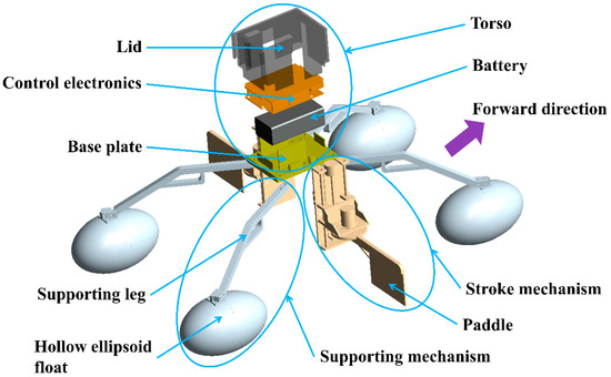
Figure 1.
The structure of the water strider robot.
2.2. Design of the Supporting Mechanisms
The supporting mechanisms consist of four pairs of supporting leg and hollow ellipsoid float. Each supporting leg is a square strip that is bent at 150° in the middle and it is mounted on the base plate at 30° to the robot’s forward direction (Figure 1). This design makes the supporting mechanisms stretch over the water surface while keeping the torso high away from the water surface. A kind of hollow rotational ellipsoid was selected as the float for the supporting mechanism, because it has good hydrodynamics compared with several other common shapes (e.g., sphere or cone) [20]. Four pairs of the supporting leg and the float were installed symmetrically around the robot with a long axis of the float along the forward direction of the robot. The float is 32.5 mm in short radius and 52.5 mm in long radius, and can generate a maximum buoyancy of ~2.2 N. A maximum buoyancy of 8.9 N was generated by the robot which is strong enough to withstand the weight of the entire robot and has a load capacity of ~3.9 N. Compared with a mechanism that relies on water surface tension, this supporting mechanism has much stronger load capacity and is more robust in adapting to complicated water surface conditions. Additionally, the load capacity can be readily adjusted by changing the size of the float, to meet different application requirements.
2.3. Design of the Stroke Mechanisms
The water strider can not only move in a straight line, but also make a turning. To achieve a similar function, two paddles driven by two stepper motors equipped with the corresponding reducers (1.61.123.003.00, Bühler Motor GmbH, Nuremberg, Germany) were used to control the movement of the entire robot. They were the same and symmetrically mounted on either side of the robot torso, which greatly simplified the motion control strategy of the robot. For example, the forward or backward motion could be realized by making the two paddles simultaneously rotate at the same speed and in the opposite rotational direction. Whereas, the turn motion can be achieved by simply setting the same rotational direction for the two paddles. The stepper motors drive the paddles rotating on the horizontal plane and generate propulsion for the robot when the paddles are immerged into the water. The stepper motor rotates according to the step angle. Compared with the direct current (DC) motor, its angular velocity would not change significantly when the paddle strokes the water. Since the surface of the paddle is always perpendicular to the water surface, it does not generate a vertical force which is conducive to the motion stability and efficiency of the robot.
As stated above, the stroke mechanism will not provide propulsion if only part of the paddle is submerged in the water. However, determined by working mode of the stepper motor, the paddle must turn back to the starting position from the end of one stroke action before it can do the next stroke action. The entire paddle must be lifted up from the water during this process otherwise it will block the current motion of the robot. Therefore, a linear guide mechanism was designed to control the paddle moving in and out of the water. The linear guide mechanism was driven by a linear stepper motor (SM1589, Nidec Corporation, Kyoto, Japan), and the movement of the stroke mechanism was constrained along two guide rods to keep the movement as steady as possible (Figure 2). In general, the movement of the paddle was controlled by the combination of the linear stepper motor and the stepper motor.
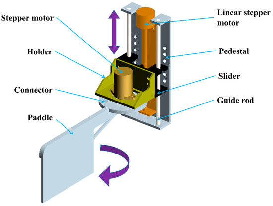
Figure 2.
Computer aided design (CAD) model of the stroke mechanism. The two purple arrows represent the movement of the stroke mechanism on the vertical and horizontal planes.
3. The Kinematics Analysis of the Stroke Mechanism
The mechanical structure of the stroke mechanism provides a hardware basis for the movement of the paddle. However, the way in which the stepper motor and the linear stepper motor cooperate with each other to make the stroke mechanism generate an ellipse-like spatial trajectory still needs to be analyzed. The kinematics of the stroke mechanism also influenced the hydrodynamic modeling of the robot, as seen in the next section. Although we have already analyzed the kinematics of the stroke mechanism in our previous work [25], here we use a relatively easier method to analyze its kinematics in more detail.
The stroke mechanism is a linear guide and rotation coupled mechanism which could be simplified as a double joint mechanism with two degrees of freedom. The spatial position of a point on the paddle with reference to the nonmoving part of the robot itself is determined by the angle and position between the joints (i.e., the linear stepper motor and the stepper motor). Therefore, two Cartesian coordinate systems were established to describe the position of any point on the paddle relative to the torso of the robot which is simpler than the method of using three coordinate systems in the conference paper. A local coordinate system was built on the paddle to describe the coordinate value of any point on the paddle. A global coordinate system was built on the base plate to depict the movement of the local coordinate system. By a homogeneous coordinate transformation [26], the coordinates of any point on the paddle in the local coordinate system can be converted to the global coordinate system.
The center of the upper surface of the base plane o was set as the origin of the global coordinate system labeled coordinate system O (Figure 3). The paddle was simplified as a face in this study since it was very thin. The intersection of the rotation axis and the top edge of the paddle q was set as the origin of the local coordinate system, labeled coordinate system A. The two origins overlapped with an offset of a in the horizontal direction and b in the vertical direction. Since points on the paddle rotate around the same axis (i.e., the axis of the stepper motor) and move along the linear guide mechanism, the movement trajectories of the points are similar. For any point M on the paddle, its position in the local coordinate system A is constant and is expressed as (0, y0, z0, 1) and the position of point M in the global coordinate O is (0, y0 + a, −b − z0, 1). When the paddle rotates and moves up or down, the position of the point P in the global coordinate system O is given by
where b1 is the displacement of the paddle in the vertical direction and , ω1 is the angular velocity of the linear stepper motor, P1 is the pitch of the screw (i.e., 3 mm), t is running time, θ is rotational angle of the paddle and , ω2 is the angular velocity of the stepper motor with the reducer. By replacing b1 with , and replacing θ with , Equation (1) can be rewritten as
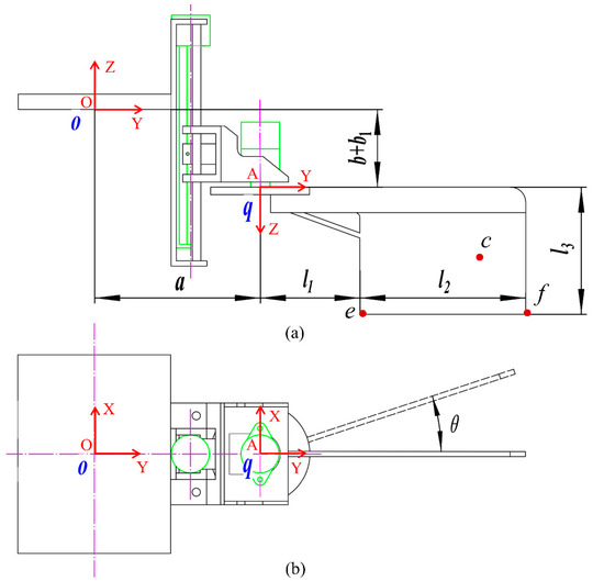
Figure 3.
Front and top view of the stroke mechanism: (a) the front view; (b) the top view. In the initial state (i.e., after the robot is assembled and before it runs), for the coordinate system O and A, the X and Y positive axis horizontally extend on the paper, and horizontally extend to the right, respectively. The Z positive axis vertically extends upward and downward for coordinate system O and coordinate system A, respectively. b1 is the displacement of the paddle in the vertical direction.
According to Equation (2), the paddle can produce many different ellipse-like spatial trajectories such as a water strider by controlling the velocities of the stepper motor and the linear stepper motor. It is difficult to study all ellipse-like spatial trajectories, so this article selects a trajectory for research based on the robot structure and hydrodynamics of the paddle which allows the paddle to generate as much power as possible. In the vertical direction, considering the length of the screw in the linear stepper motor, the maximum displacement of the paddle b1 was set as 4.8 cm. When the paddle moves down 2.4 and 4.8 cm from the top of the screw, the bottom of the paddle contacts the water surface and reaches the maximum depth in the water, respectively. Because the minimum step angle of the linear stepper motor was large (i.e., 20°), the speed of the paddle was set as a constant to smooth the movement of the paddle. According to the hydrodynamic analysis of the paddle, it was found that the greater the rotational angle, the greater the area of the resistance generated by the paddle. So the rotational angle of the paddle θ is limited to −60°~60° to ensure that the paddle generates thrust rather than drag most of the time. The rotational angle was symmetrically distributed on the front and rear parts of the robot in the horizontal direction. Because the angular resolution of the stepper motor and the reducer combination could be small (i.e., 0.87°), the paddle would rotate still smoothly even if the angular velocity of the stepper motor is segmented into several parts to improve the performance of the paddle. A larger angular velocity of the stepper motor was set to the paddle when the paddle nears θ = 0 to increase the propulsion of the robot; a lower angular velocity of the stepper motor was set to the paddle when the paddle nears θ = 60° and θ = −60° where the rotational direction of the paddle has changed; a middle velocity was set to the paddle when the paddle was in other positions. If the angular velocities of the stepper motors are too high, they would lose step which affect the stroke trajectory of the paddle. Figure 4 is a scheme of the velocities of the two motors and the stroke cycle T is 1.6. The velocities were close to the limit of the motors without losing step. So we should control the motors to not exceed the velocities shown in Figure 4 to ensure the accuracy of the stroke trajectory. The stroke speed of the paddle can be adjusted by modifying the stroke cycle. The velocities of the motors can be set according to the velocity ratio shown in Figure 4, so as to ensure the stroke trajectories of the paddle are the same in different stroke cycles. For convenience, the stroke cycle T was used to characterize the stroke speed of the paddle.
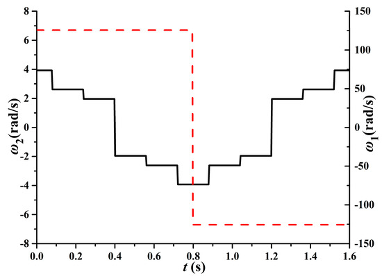
Figure 4.
Angular velocities of the linear stepper motor ω1 (the dashed red line) and the stepper motor ω2 (the solid black line) as a function of time t when the stroke cycle T is 1.6 s.
Since the stroke trajectories of the paddle in different stroke cycles are the same, we took the movement of the paddle with the stroke cycle being T = 1.6 s as an example to analyze the stroke trajectory. For all points on the paddle, their movements were the same in the vertical direction and similar in the horizontal direction since they rotate along the same rotation axis. Point e and point f are the two vertices at the bottom of the paddle which were in the innermost loop and the outermost loop of the stroke trajectory when the paddle rotates, respectively. The trajectory curves of two points can describe the stroke trajectory of the paddle at two extreme positions and we chose point c (Figure 3) on the inner surface of the paddle to describe the general stroke trajectory of the stroke mechanism. The coordinates of points e, f, and c in coordinate system A are (0, 35, 50, 1), (0, 100, 50, 1), and (0, 73, 24, 1), respectively. By substituting the ω1 and ω2 in Equation (2) with the values shown in Figure 4 and the movement trajectories of points e, f, and c in a stroke cycle, Figure 5 was obtained according to a numerical simulation calculated by the MATLAB software (The MathWorks, Inc., Natick, MA, USA). The trajectory curves of points e, f, and c infer that the paddle or the stroke mechanism can form an ellipse-like spatial trajectory. Here, the displacement between the two farthest points on the horizontal plane (i.e., the XY plane in Figure 5) in the trajectory curve of point f can represent the stroke length of the paddle. Compared to the length of the paddle, the stroke length was large (173 mm) which was conducive to the work of the robot.
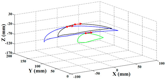
Figure 5.
The trajectory curves of points e, f and c. The blue, green and black lines represent the curves of points f, e, and c, respectively. The red points and arrows, respectively, are the initial positions and initial directions of the points.
4. Hydrodynamic Modeling and Analysis of the Robot
In the previous two sections, the structure of the water strider robot’s design is provided and the movement of the paddle is analyzed. Hydrodynamic modeling is an efficient, comprehensive approach to represent the dynamics and motion of a robot in fluid. It can calculate the hydrodynamic characteristics of the robot including the propulsion, resistance, and speed of the robot, which are important for the analysis of the robot’s motion performance, power, and efficiency. In the following content, firstly, a semiempirical general hydrodynamic model is established. Secondly, the coefficients related to the hydrodynamic model are solved. Finally, the hydrodynamic characteristics, power, and efficiency of the robot are studied to prove that the robot adopting an ellipse-like spatial stroke trajectory is beneficial to the moving efficiency.
4.1. Hydrodynamic Modeling
The water strider robot mainly focuses on a forward motion in practical applications, therefore, only the hydrodynamic model of the robot when the robot performs a forward motion has been studied. Because it would be complicated to consider all the circumstances, this study intended to start with a simplification. We assumed that the flow direction of the water was consistent with the motion direction of the robot and the rate of the water was steady. The propulsion was produced by the interaction between the paddles and the water when the paddles rotate. This process produced some resistance when the linear velocity of some parts of the paddles near the shaft were slower than the speed of the robot. The other resistance came from the four floats on the supporting mechanisms contacting the water surface when the robot moved.
To reduce the resistance generated by a paddle, a rectangle corner near the shaft (i.e., the r, u, q, e area in Figure 6) was cut from the paddle. This ensures the linear velocity of the rest paddle immersed in the water will be greater than the speed of the robot. Meanwhile, a rib was added to enhance the stiffness of the paddle. In Section 4.3, it is proved that cutting the rectangle corner can increase the speed of the robot. The force generated by the paddle can be divided into a thrust and a lift (Figure 7) [27]. For the forward motion of the robot, the driving force of the robot was determined by the resultant force of the two paddles immersed in the water. In the direction perpendicular to the forward direction of the robot, the two paddles generating the lift forces were equal in magnitude and opposite in direction, so they cancel each other out. In the forward direction of the robot, the two paddles generating the thrust forces were equal in the magnitude and same in the direction, so the sum of the thrust forces was the driving force of the robot. The thrust force can be calculated approximately by a formula that is used to calculate the drag force of the external flow past an object [23,24,28]. It is
where F is the resistance, C is a dimensionless coefficient which is determined by the shape of the object and the surface condition, ρ is the fluid density, A is the part of area that the object immerses in water and projects in the plane perpendicular to the forward direction of the object, and V0 is the relative velocity between the object and the water. This formula cannot be used directly to calculate the thrust of the paddle, because the linear velocity of each point on the paddle is different. To get around this limitation, a differential method was adopted to divide the entire paddle into many infinite sections along the radial direction of the shaft, and the integration of the force of each infinite section was used to approximate the thrust. The thrust of the paddle FT can be approximated as
where KT is a customized thrust coefficient and expressed as KT = CTρcosθ, CT is the dimensionless coefficient in the thrust calculation which is related to θ, θ is the rotational angle of the paddle (Figure 7), ω is the rotational speed of the paddle, t is the time that the paddle is rowing, H(t) is the water line (i.e., dashed blue line in Figure 6) which represents the depth of the paddle immersed in the water, y is coordinate in the Y axis of the coordinate system A, and dy is the infinitesimal increase in the Y axis. Here, the lower and upper limit of integration (i.e., e and f) are determined by the shape of the paddle in the local coordinate system A. VT is the relative velocity between the water with the paddle which is given by
where V is the speed of the robot, |VT| is the absolute value of VT and it ensures that when VT is negative, and the force provided by paddle for the robot is the resistance. By replacing VT with Equation (5), Equation (4) can be rewritten as
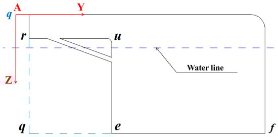
Figure 6.
The shape of the paddle in the stroke mechanism. The blue line is the water line when the paddle is immerged into the water.
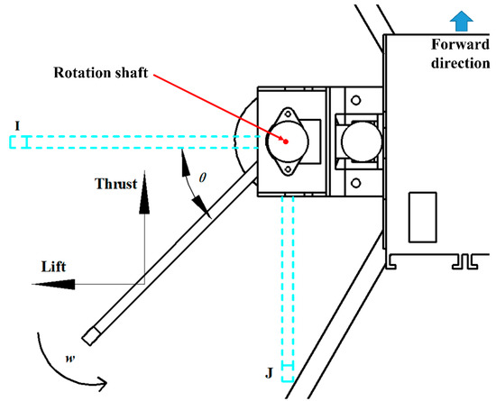
Figure 7.
The rotation of the left-side paddle while the robot advances. The approximate directions of the thrust and lift forces generated by the paddle are indicated.
Similarly, the speed of the robot in the lateral direction was zero and the lift force FL at each paddle can be calculated by
where KL is a custom lift force coefficient and expressed as KL = CLρsin θ, CL is the dimensionless coefficient in the lift calculation which is related to θ. Due to the symmetry of the robot structure, when the robot moves forward, it only produces three kinds of motions: surge motion in the forward direction, heave motion in the vertical direction, and pitch motion. Since the supporting mechanisms spread out on the water surface to make the robot stand stalely, the pitch motion of the robot can be ignored. The paddle is always perpendicular to the water surface which is considered to not produce vertical force, so the heave motion of the robot is mainly affected by the supporting mechanisms. Similar to the hydrodynamics of a ship or an AUV, and under the assumption that the water is always calm, the drag force FR in the forward direction provided by the supporting mechanisms is
where FD is the viscous hydrodynamic force, FM is the inertia hydrodynamic force related to the added mass, KD, KD1, KD2, XW, and XWW are viscous hydrodynamic coefficients, W is the vertical velocity of the robot, U0 is the work point of the robot, MV is the added mass of the robot. The work point U0 is the speed of the robot we specify, which affects values of some viscous hydrodynamic coefficients. In this paper, the relevant viscous hydrodynamic coefficients are measured under the drive of a motor in Section 4.2.1 and the work point U0 is the speed of the motor. The force FB in the vertical direction provided by the supporting mechanisms is
where Z0, ZV, ZW, ZVV, and ZWW are the viscous hydrodynamic coefficients in the vertical direction, MW is the added mass of the robot in the vertical direction, ξ is the displacement of the robot in the vertical direction, Zξ and Zξξ are the hydrodynamic coefficients related to the gravity and buoyancy of the robot. The water surface was near the largest cross-section of the ellipsoid floats which had a greater damping effect on the heave motion of the robot. In order to simplify the analysis, the effect of the heave motion on the surge motion of robot were ignored (i.e., the terms XWW and XWWWW in Equation (9) are ignored). Since the heave motion is not the focus of this article and requires lots of work to obtain the relevant hydrodynamic confidents, we will not further analyze the vertical motion of the robot. Based on Newton’s second law, Equations (6) and (8)–(10), the general hydrodynamic model of the robot in the forward direction is
where m is the weight of the robot. Equation (12) represents the relationship between the hydrodynamics and motion of the robot. The general hydrodynamic model can represent all forward motions of the robot. According to the instantaneous power in the dynamics, the power of robot provided by the two paddles P can be expressed as
Using the power that can promote the robot forward motion as the effective power, the efficiency of the paddles η can be expressed as
When the stroke action of the paddles is determined, the robot would eventually reach a dynamic balance since the force generated by the paddles is not a constant. It means that the final speed of the robot periodically oscillates and the power of the paddles changes periodically. Studying the average power and efficiency in a stroke cycle when the robot reaches a dynamic balance is more meaningful. The average power P0 in a stroke cycle can be calculated by
where t0 is the chosen initial time when the robot reaches the dynamic balance. The efficiency in a stroke cycle can be calculated by
4.2. Coefficients Evaluation of the Hydrodynamic Model
It needs be highlighted that there are several coefficients in the hydrodynamic model (i.e., KT, KL, KD, and MV) still pending which should be approximated to facilitate the application of the model in the following sections. Since KT = CTρcos θ—where CT and cos θ are variables related to θ, ρ is constant and KT is a variable related to θ—we can use a function to express the relationship between KT with θ. For KL, we can also use a function to express the relationship between KL with θ just as KT. KD and MV are constant. KT, KL, KD, and MV can be obtained by the computational fluid dynamics (CFD) simulation or experimental measurement and the experimental measurement can make the measured coefficients closer to the actual situation. Here KT, KL, and KD are obtained by an experimental method. MV is obtained by the CFD simulation since it is not easy obtained through the experimental measurement.
4.2.1. KT, KL and KD Measurement
A quasi-static approach [27,29] was adopted to determine the relationship between KT with θ and the relationship between KL with θ. According to Equation (6), when the paddle moves straight on the water at a fixed angle and a fixed water line H(t) = h, the generated force Fe can be expressed as
where Vm is the speed of the paddle, xef is the distance of point e to point f. We can measure different values of Fe when setting the immobile paddle at different angles θ. From Equation (17), we can get different values of KT when the immobile paddle is at different angles θ. Using this static measurement relationship between KT and θ to represent the relationship between the dynamics of KT and θ when the paddle rotates is a quasi-static approach. The relationship between KT and θ is not continuous because the data Fe corresponding to θ obtained by the experiment are not continuous and it cannot represent a real condition when the paddle rotates on the water. Therefore, we used these data to fit a continuous appropriate function KT = f(θ) to indicate the relationship between KT and θ. The KT measured when the immobile paddle was set at angle θ was equal to the KL measured when the immobile paddle was set at angle π/2 − θ. The function relationship between KL and θ can be expressed as KL = f (π/2 − θ). So we can get the relationship between KL and θ according to the function relationship between KT and θ. KD = FD/V2, which can be obtained by Equation (9) and KD can be determined when FD and V are measured according to the experiment.
In order to get the function relationship between KT and θ, a stent was fixed on the slider and the stent was connected to the paddle by a 3-axis force sensor (MX020-10N, NMB, Japan) (Figure 8a). When the motor drove the slider, the paddle moved with the slider and slid on the water. The generated force was measured by the force sensor. The speed of the dragging motor was set to 26 cm/s considering the length of the guide (1.5 m) and the force generated by the paddle. Because the paddle was always perpendicular to the horizontal plane, the force sensor measured the horizontal force of the paddle in the moving direction. The sensor measured the average forces of paddle Fe when it slid with different angles θ in a sink. A total of 19 groups of Fe and θ combinations were tested when θ increased from 0° to 90° with the angular interval of 5°.
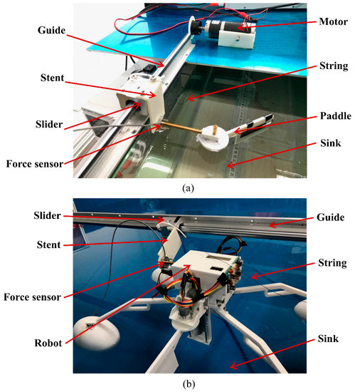
Figure 8.
Pictures of the parameter measurement experiment: (a) KT measurement experiment; (b) KD measurement experiment.
The data recorded different θ corresponding to Fe measured in the experiment are shown in Figure 9. According to Equation (17), the KT corresponding to different angles θ has been calculated (i.e., points in Figure 10). A quadratic polynomial function was used to fit these points to get a continuous relationship between KT and θ because the quadratic polynomial function is simple and its function curve conforms to the image formed by the data. The fitted curve is shown in Figure 10 and Equation (18) is the fitting function:
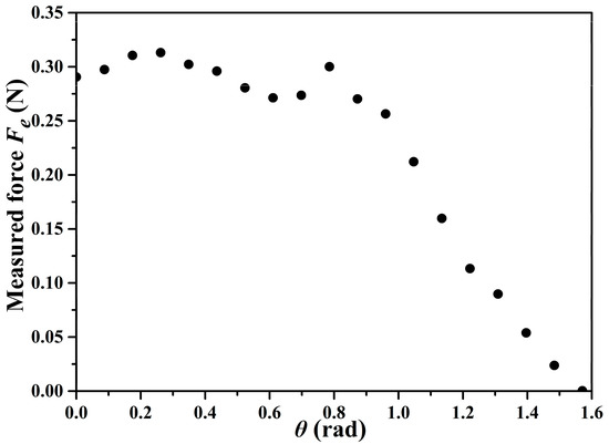
Figure 9.
The measured Fe as a function of the angle of the paddle θ.
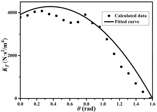
Figure 10.
The value of KT as a function of the angle of the paddle θ. Points are the values of KT by calculation and cure is the fitted cure of KT.
The function relationship between KL and θ is expressed as KL = f (π/2 − θ). Through Equation (18), we can get the relationship between KL and θ as
Figure 8b shows the experiment for measuring the viscous hydrodynamic force FD when it was dragged moving on the water by a motor at a speed of VD which was similar to the previous experimental method. The speed at which the motor dragged the slider was also set to VD = 26 cm/s and the average drag force FD measured by the sensor was 0.115 N. The KD could be obtained by KD = FD/V2 and was calculated as equal to 1.70 N∙s2⁄m2.
4.2.2. MV Measurement
MV is the added mass of the robot and was measured by a CFD simulation here. In the CFD simulation, the hydrodynamic coefficient measurement of an underwater robot was mainly carried out by planar motion mechanism (PMM) tests. A PMM test can obtain the functional relationship between the drag force and time of a robot by forcing the robot to perform periodic oscillations in a fixed direction. By performing a Fourier transform on the functional relationship, the hydrodynamic coefficient parameters such as the acceleration term and velocity term can be obtained [30]. In order to obtain the added mass of the robot in the forward direction, the robot was forced to perform a periodic pure surge motion in the robot forward direction. The displacement , velocity , and acceleration of the robot are given by following equations:
where α is the amplitude and β is the circular frequency of the surge motion. Here α is set as 0.04 m and β is set as 0.8π. Ignoring the effect of air on the robot and the four ellipsoid floats immersed in the water, we can solve the added mass by calculating the hydrodynamic force of the four ellipsoid floats. Unlike the underwater robot which was completely in the water, the four ellipsoid floats were approximately half in the water and half in the air. A two-phase flow CFD model was used to study their hydrodynamics. Since the effect of air on the robot was neglected, the air domain was added on the CFD model only to simulate the conditions of the four floats on the gas–liquid surface and the force of the floats acted by the air was not calculated. The two-phase flow CFD model in the COMSOL software (COMSOL Inc., Stockholm, Sweden) is shown in Figure 11.
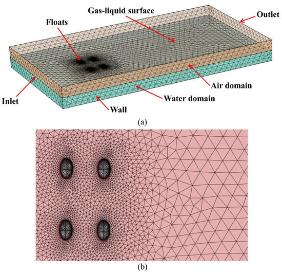
Figure 11.
The computational fluid dynamics (CFD) two-phase flow model in COMSOL software: (a) overall of the model; (b) the area around the floats.
The model uses an unstructured mesh method. The upper part of the model is the air domain (3.4 m × 1.8 m × 0.2 m) and the lower part is the water domain (3.4 m × 1.8 m × 0.2 m). The left boundary is the velocity inlet and the inflow velocity U is set as 0.1 m/s. The right boundary is the pressure outlet and pressure is set as 0. The other boundaries of the air domain and the water domain were set as no slip wall. The four floats were in the gas–liquid surface and exhibited a periodic surge motion in a direction perpendicular to the inflow direction. The motion of four floats were defined by the moving mesh method in the COMSOL software. The Reynolds number of the CFD model Re can be calculated by
where d is the long diameter of the float and μ is the viscosity of the water. By calculation, the Reynolds number is 10,500 and a RANS k-ε turbulent model was used in the CFD simulation. The force of the four floats in the robot forward direction can be exported from the COMSOL software and is shown in Figure 12. The model was calculated by using 384,965 meshes and 239,690 meshes. It was found that the results of the double calculations were similar and the results were independent of the number of meshes. The relationship between the force FI and time t in the Figure 12 can be fitted by
where is the velocity-based coefficient and is the acceleration-based coefficient. Here, the coefficient is equal to the added mass MV which is 0.083 by calculation. The value is close to the theoretical value of 0.116 [31]. In addition to the difference between the calculated and theoretical values from the CFD simulation calculation error, the two-phase flow model used to imitate the condition of half the ellipsoid floats immersed in the water was different from the model of the ellipsoid floats completely immersed in the water. The simultaneous CFD simulation of four ellipsoid floats in water was different from the CFD simulation of a single ellipsoid float in water which also had an impact on the simulation result.
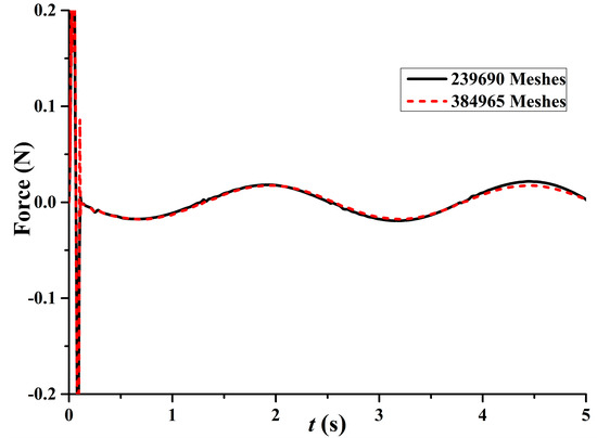
Figure 12.
The force acting on the four ellipsoid floats in the water as a function of t at two different mesh numbers.
4.3. Hydrodynamic Analysis for the Robot
In the previous two sections, the general hydrodynamic model of the robot is established and the coefficients in the model are solved. In this section, the hydrodynamic characteristics of the robot when it performs the ellipse-like spatial stroke trajectory is studied. Below we derive the hydrodynamic model for when the robot performs the ellipse-like spatial stroke trajectory from the general hydrodynamic model. According to the kinematics analysis of the paddle in Section 3, The water line H(t) in Equation (12) when the robot performs the ellipse-like spatial stroke trajectory becomes
ω and θ in Equation (12) should be replaced by ω2 and , respectively. Therefore, the hydrodynamic model when the robot performs the ellipse-like spatial stroke trajectory is
From the numerical simulation of Equation (26) calculated by the MATLAB software, the speed of the robot in different stroke cycles T is shown in Figure 13. The result denotes that the robot reaches the dynamic balance after going through three stroke cycles. The final speed of the robot fluctuates periodically around a constant value just as we predicted. The average speeds of the robot in the stroke cycles of 1.6, 2.0, 2.4, 2.8, and 3.2 s were 0.108, 0.087, 0.075, 0.059, and 0.050 m/s, respectively, when it reached a dynamic balance. As the stroke cycle T increases, the speed of the robot decreases. In order to verify the effect of the rectangular corner on the paddle and the stroke efficiency of the paddle in the following content, the movement of the paddle with the stroke cycle T = 1.6 s was used as the research object. In Section 4.1, a rectangle corner near the shaft of the paddle was cut to reduce the resistance generated by the paddle. In order to prove this, a case in which the robot has two intact paddles was conducted as a numerical simulation. The intact paddles performed the same movement as the paddles with a rectangular piece cut out of the corner and the stroke cycle was T = 1.6 s. In this case, the hydrodynamic model of the robot can be easily derived from Equation (12) and is omitted here. The speed of the robot with two intact paddles is shown in Figure 14. It can be found that the speed of the robot with two intact paddles was lower than the robot with the paddles with a rectangular piece cut out of the corner. This explains that cutting off a rectangular piece from the corner near the shaft from the paddles can increase the thrust of the robot.
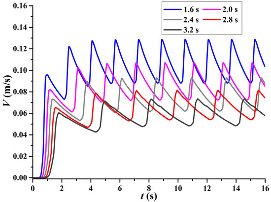
Figure 13.
The speeds of the robot as a function of time t in different stroke cycles T. The blue, pink gray, red, and black lines are the speeds of the robot when the stroke cycles are 1.6, 2, 2.4, 2.8 and 3.2 s, respectively.
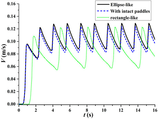
Figure 14.
The speeds of the robot as a function of t at different situations. The solid black line is the speed of the robot when it performs an ellipse-like spatial stroke trajectory; the dashed blue line is the speed of the robot when it performs an ellipse-like spatial stroke trajectory with two intact paddles; the dotted green line is the speed of the robot when it performs a rectangle-like spatial stroke trajectory with two intact paddles.
In order to evaluate the stroke efficiency of the robot when it performs the ellipse-like spatial stroke trajectory, another case was set up for comparison. In this case, the vertical translation and rotational movements of the paddle were alternating, but the vertical translation speed and rotational speed of the paddle were the same as the robot when it performs the ellipse-like spatial stroke trajectory. The paddle in this case performed a rectangle-like spatial stroke trajectory and the cycle changed to 3.2 s. The hydrodynamic model of the robot when the paddles performed a rectangle-like spatial stroke trajectory can be derived from Equation (12) and the speed of the robot in this case is shown in Figure 14. The speed when the robot performed an ellipse-like spatial stroke trajectory was faster than when it performed a rectangle-like spatial stroke trajectory. Below, we compare the two kinds of stroke action in terms of power and efficiency. The power calculation formulas of the robot for the two stroke methods can be derived from Equation (13). The powers under different stroke methods are shown in Figure 15 which clarifies that the robot adopted a rectangle-like spatial stroke trajectory required more energy during the interaction between the paddles and the water. Calculated by Equation (15), the average powers when the robot performed the ellipse-like spatial stroke trajectory and the rectangle-like spatial stroke trajectory were 6.52 × 10⁻³ W and 5.25 × 10⁻³ W, respectively. It means that the paddle performing an ellipse-like spatial stroke trajectory can provide more power for the robot at the same rotational speed of the paddle. Calculated by Equation (16), the efficiencies when the robot performed the ellipse-like spatial stroke trajectory and the rectangle-like spatial stroke trajectory were 0.880 and 0.751, respectively. This means that the generated power can be better applied to the robot motion when the paddle performs an ellipse-like spatial stroke trajectory. Whether it is from the perspective of the speed or the stroke efficiency of robot, it clarifies that an ellipse-like spatial stroke trajectory can improve the moving efficiency of the robot.
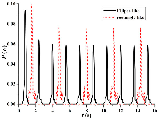
Figure 15.
The powers of the robot P when the paddles perform an ellipse-like spatial stroke trajectory and rectangle-like spatial stroke trajectory as a function of the running time t.
5. Experimental Verification
The structural design and hydrodynamic characteristics of the water strider robot have been studied. In order to verify the results of these studies, this section will verify the two important aspects of the robot designed in this paper, namely, the stroke mechanism which can create an ellipse-like spatial stroke trajectory and the mobility of the robot as well as the hydrodynamic model.
5.1. Verification of the Stroke Trajectory Curve
The curve of point f is easy to observe in the experiment and it is representative to use this point to represent the stroke trajectory of the robot since the trajectory of all points on the paddle is similar. The trajectory curve of point f on the vertical plane (e.g., the XZ plane in the absolute coordinate system O) can be recorded by a camera from which the X and Z coordinates can be obtained. The Y coordinate of point f can also be acquired by |X/tanθ| + a which can be derived from Equation (2). The spatial trajectory of point f can be obtained from the X, Y, and Z coordinates. Here it is convenient to use the stroke trajectory curve on the vertical plane of point f to represent the spatial stroke trajectory curve of point f because the stroke trajectory curve on the vertical plane can reflect the characteristic of the ellipse-like trajectory.
Since the stoke trajectories of the paddle in different stroke cycles T are the same, the paddle with the stroke cycle T = 1.6 s is tested. In order to verify the stroke trajectory of point f in Figure 5, the angular velocity of the stepper motors and the linear stepper motors were set to be theoretically consistent (Figure 4) in the experiment. However, the rotation directions of the stepper motors on the two stroke mechanisms were set to be opposite to each other to ensure the robot’s locomotive progress. The robot was placed on the water surface of a tank which was made of transparent Plexiglass and a CCD camera was placed horizontal to the robot outside the tank to record the motion of the robot and stroke action of the one side stroke mechanism (Figure 16). According to the video, the position of point f relative to the torso was analyzed frame-by-frame.
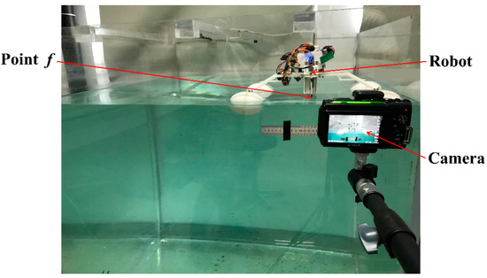
Figure 16.
The experimental record of the stroke mechanism sliding on the water from the viewpoint of one side.
Figure 17 is the experimental and theoretical trajectory curves of point f on the X–Z and Y–Z plane. From Figure 17a, the experimentally measured curve is similar to the theoretical curve which is very similar to an oval. It shows that this stroke mechanism can simulate the real water strider insect to produce an ellipse-like spatial trajectory in practical applications when the stroke mechanism rows in the water. The theoretical and experimental curves in the above part are very consistent, and the theoretical and experimental curves in the below part produce a little error. This error arises from two aspects. (1) The blow part curve is the process in which the paddle strokes the water and fluctuations in the water surface cause the robot to sway. (2) The refraction phenomenon of the paddle image is transmitted from the water into the CCD camera in the air, which causes error in the mapping of the stroke trajectory curve.
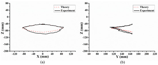
Figure 17.
Experimental and theoretical trajectory curves of point f: (a) in X–Z plane; (b) in Y–Z plane.
5.2. Verification of the Robot Mobility as Well as the Hydrodynamic Model
The locomotion of the robot was examined in the stroke cycle of T = 1.6 s when the paddles performed an ellipse-like spatial stroke trajectory continually. The length of the pool was 3 m and its width was 2 m. The robot completed two different motions, going straight and turning. Similarly, the angular velocities of the stepper motors and the linear stepper motors were set to be the same as shown in Figure 4. When the robot went straight and turned, the rotational directions of the stepper motors on the stroke mechanisms on both sides were set to be opposite and the same, respectively. Figure 18 is the path of the robot’s locomotion progress within 6 s when the robot reached a dynamic balance. It can be seen that the trajectories of five feature points on the supporting legs and the center of the robot are almost straight lines, which shows that the robot has a good marching ability and can perform in a straightforward motion. By calculating the distance traveled by the robot in 6 s, the average speed of the robot moving forward was 0.129 m/s. By comparing the body-length of the robot, the robot can reach 0.39 BL/s. Figure 19 shows photo snapshots of the robot turning right within 8 s. It can be seen that the robot rotates almost around its own center. The robot turned 180° in 8 s, thus the turn speed is 22.5°/s. The two figures show that whether the robot goes straight or turns, the robot has good mobility.
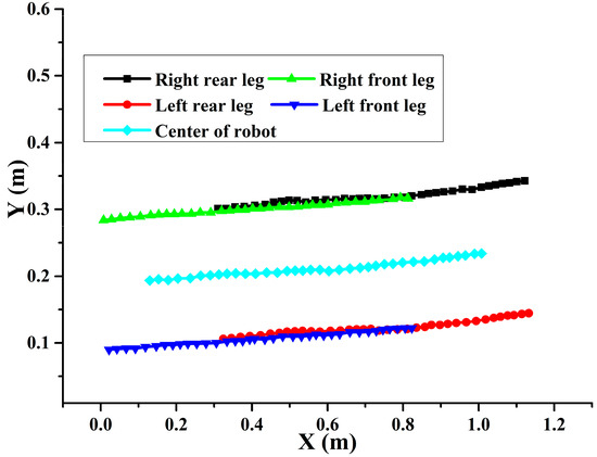
Figure 18.
The path of the robot’s progress locomotion within 6 s. The five lines express five feature points on the legs and the center of the robot.
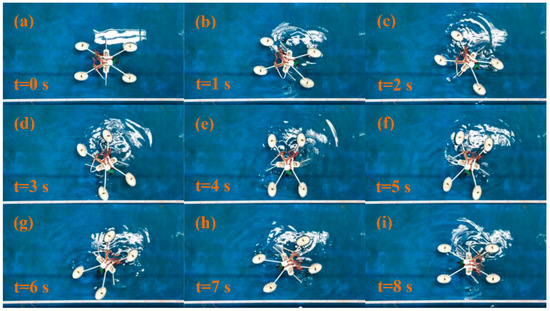
Figure 19.
The positions of the robot at different times t: (a) 0 s, (b) 1 s, (c) 2 s, (d) 3 s, (e) 4 s, (f) 5 s, (g) 6 s, (h) 7 s, and (i) 8 s, when the robot is turning right.
In addition to testing the robot motion with a stroke cycle of 1.6 s, we also conducted forward motion experiments on the robot with the stroke cycles of 2.0, 2.4, 2.8, and 3.2 s. According to different stroke cycles, the angular velocities of the stepper motors and the linear stepper motors were set with reference to the velocity ratio in Figure 4. Figure 20 shows photo snapshots of the robot moving forward within 6 s when the stroke cycle is T = 2.0 s. The displacement of the robot was measured by the ruler next to it. By recording the motions of the robot in other stroke cycles, the average speeds of the robot in different stroke cycles T can be calculated—shown in Figure 21. It can be found that the speeds of the robot measured by the experiments are relatively close to the theoretical value which proves the applicability of the hydrodynamic model.
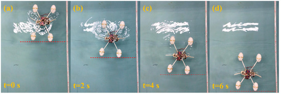
Figure 20.
The positions of the robot at different times t: (a) 0 s, (b) 2 s, (c) 4 s, and (d) 6 s, when the robot is moving forward with the stroke cycle T = 2.0 s.
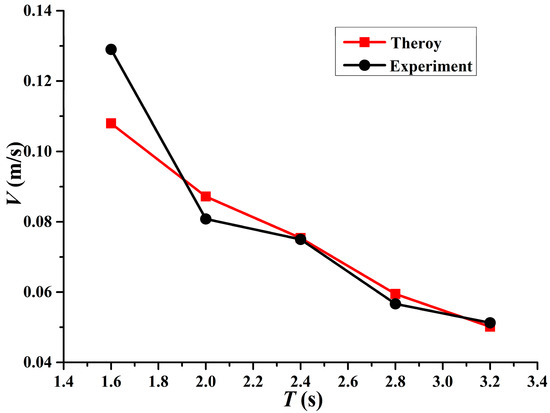
Figure 21.
Theoretical speeds and experimental measurement speeds of the robot in different stroke cycles T.
6. Conclusions
A new buoyancy-supported water strider robot was proposed. Its stroke mechanism is composed of a linear guide and rotation coupled mechanisms which can produce an ellipse-like spatial trajectory as well as a real water strider. We establish a semiempirical hydrodynamic model for the robot. Since the stroke mechanism of the robot is not a common drive, the established hydrodynamic model is meaningful and innovative. According to the analysis of the hydrodynamic model, it finds that the robot performing an ellipse-like spatial stroke trajectory favors moving efficiency. We can predict the speed of the robot according to the stroke cycle of the paddle which can guide the design of the robot speed control system. The hydrodynamic model is also instructive for the optimization of the robot structure, efficiency, and stroke trajectory to make the robot exhibit a better motion performance. The experiments verify that this stroke mechanism can produce an ellipse-like spatial trajectory similar to a real water strider in practical applications and the robot has good mobility whether it goes straight or turns. The theoretical value of the robot speed is relatively close to the experimental value which indicates that the hydrodynamic model established in this article is applicable. The method to establish a hydrodynamic mode to study the hydrodynamic characteristics of a water strider robot may provide some inspiration for other similar water surface robots, especially robots driven by the paddles. This article only considers the hydrodynamic characteristics of a robot when it moves forward. The turn hydrodynamic characteristics of robots will be studied in future work.
Author Contributions
The individual contributions of authors: conceptualization, H.H., and C.S.; methodology, C.S.; software, Y.S.; validation, C.S., and G.W.; formal analysis, H.H., H.W., and C.S.; data curation, Y.S. and G.W.; writing—original draft preparation, C.S.; writing—review and editing, H.H., and H.W.; visualization, H.H., H.W. and C.S.; supervision, H.H., and H.W. All authors have read and agreed to the published version of the manuscript.
Funding
This research received no external funding.
Conflicts of Interest
The authors declare no conflict of interest.
References
- Wang, K.; Ma, Y.; Shan, H.; Ma, S. A snake-like robot with envelope wheels and obstacle-aided gaits. Appl. Sci. 2019, 9, 3749. [Google Scholar] [CrossRef]
- Nguyen, Q.V.; Chan, W.L. Development and flight performance of a biologically-inspired tailless flapping-wing micro air vehicle with wing stroke plane modulation. Bioinspiration Biomim. 2018, 14, 016015. [Google Scholar] [CrossRef] [PubMed]
- Li, H.; Liu, W.; Fu, X.; Bonsignori, G.; Scarfogliero, U.; Stefanini, C.; Dario, P. Jumping like an insect: Design and dynamic optimization of a jumping mini robot based on bio-mimetic inspiration. Mechatronics 2012, 22, 167–176. [Google Scholar] [CrossRef]
- Picardi, G.; Laschi, C.; Calisti, M. Model-based open loop control of a multigait legged underwater robot. Mechatronics 2018, 55, 162–170. [Google Scholar] [CrossRef]
- Yang, W.; Zhang, W. A worm-inspired robot flexibly steering on horizontal and vertical surfaces. Appl. Sci. 2019, 9, 2168. [Google Scholar] [CrossRef]
- Goodwyn, P.; Wang, J.; Wang, Z.; Ji, A.; Dai, Z.; Fujisaki, K. Water striders: The biomechanics of water locomotion and functional morphology of the hydrophobic surface (insecta: Hemiptera-heteroptera). J. Bionic Eng. 2008, 5, 121–126. [Google Scholar] [CrossRef]
- Sun, P.; Zhao, M.; Jiang, J.; Zheng, Y. The study of dynamic force acted on water strider leg departing from water surface. AIP Adv. 2018, 8, 015228. [Google Scholar] [CrossRef]
- Prakash, M.; Bush, J.W.M. Interfacial propulsion by directional adhesion. Int. J. Non-Linear Mech. 2011, 46, 607–615. [Google Scholar] [CrossRef]
- Song, Y.S.; Sitti, M. Surface-tension-driven biologically inspired water strider robots: Theory and experiments. IEEE Trans. Robot. 2007, 23, 578–589. [Google Scholar] [CrossRef]
- Yan, J.H.; Zhang, X.B.; Zhao, J.; Liu, G.F.; Cai, H.G.; Pan, Q.M. A miniature surface tension-driven robot using spatially elliptical moving legs to mimic a water strider’s locomotion. Bioinspiration Biomim. 2015, 10, 046016. [Google Scholar] [CrossRef]
- Yang, K.; Liu, G.; Yan, J.; Wang, T.; Zhang, X.; Zhao, J. A water-walking robot mimicking the jumping abilities of water striders. Bioinspiration Biomim. 2016, 11, 066002. [Google Scholar] [CrossRef] [PubMed]
- Koh, J.S.; Yang, E.; Jung, G.P.; Jung, S.P.; Son, J.H.; Lee, S.; Jablonski, P.G.; Wood, R.J.; Kim, H.; Cho, K. Jumping on water: Surface tension-dominated jumping of water striders and robotic insects. Science 2015, 349, 517–521. [Google Scholar] [CrossRef] [PubMed]
- Hu, D.L.; Chan, B.; Bush, J.W.M. The hydrodynamics of water strider locomotion. Nature 2003, 424, 663–666. [Google Scholar] [CrossRef] [PubMed]
- Suhr, S.H.; Song, Y.S.; Lee, S.J.; Sitt, M. Biologically inspired miniature water strider robot. Robot. Sci. Syst. I 2005, 1, 319–325. [Google Scholar] [CrossRef]
- Yan, J.; Yang, K.; Liu, G.; Zhao, J. Flexible driving mechanism inspired water strider robot walking on water surface. IEEE Access 2020, 8, 89643–89654. [Google Scholar] [CrossRef]
- Suzuki, K.; Ichinose, R.W.; Takanobu, H.; Miura, H. Development of water surface mobile robot inspired by water striders. Micro Nano Lett. 2017, 12, 575–579. [Google Scholar] [CrossRef]
- Fujii, S.; Nakamura, T. Development of an amphibious hexapod robot based on a water strider. In Proceedings of the 10th International Conference (CLAWAR), Singapore, 9–12 October 2007; pp. 135–143. [Google Scholar]
- Irawan, A.; Khim, B.K.; Yin, T. PSpHT a water strider-like robot for water inspection: Framework and control architecture. In Proceedings of the IEEE International Conference on Ubiquitous Robots and Ambient Intelligence, Kuala Lumpur, Malaysia, 12–15 November 2014; pp. 403–407. [Google Scholar]
- Gao, T.; Cao, J.; Gao, F.; Zhu, D. The research of a bionic robot that can walk on water surface based on water strider. In Proceedings of the International Technology and Innovation Conference, Hangzhou, China, 6–7 November 2006; pp. 2880–2885. [Google Scholar]
- Huang, H.; Zhang, S.; Chen, X.; Miao, J.; Ge, H. Design and modeling of a novel biomimetic robot inspired by water strider. Mar. Technol. Soc. J. 2016, 50, 35–44. [Google Scholar] [CrossRef]
- Peng, G.; Feng, J.J. A numerical investigation of the propulsion of water walkers. J. Fluid Mech. 2011, 668, 363–383. [Google Scholar] [CrossRef]
- Bush, J.W.M.; Hu, D.L. Walking on water: Biolocomotion at the interface. Phys. Today 2005, 38, 339–369. [Google Scholar] [CrossRef]
- Floyd, S.; Sitti, M. Design and development of the lifting and propulsion mechanism for a biologically inspired water runner robot. IEEE Trans. Robot. 2008, 24, 698–709. [Google Scholar] [CrossRef]
- Kim, H.G.; Jeong, K.; Seo, T.W. Analysis and experiment on the steering control of a water-running robot using hydrodynamic forces. J. Bionic Eng. 2017, 14, 34–46. [Google Scholar] [CrossRef]
- Wu, G.; Sheng, C.; Shen, Y.; Guo, Y.; Liu, X.; Zhang, C.; Wu, Y.; Huang, H. Structural design and stroke kinematics analysis of a water strider robot. In Proceedings of the 2018 MTS/IEEE Oceans, Charleston, SC, USA, 28–31 May 2018; pp. 1–6. [Google Scholar]
- Bloomenthal, J.; Roken, J. Homogeneous coordinates. Vis. Comput. 1994, 11, 15–26. [Google Scholar] [CrossRef]
- Caplan, N.; Gardner, T.N. A fluid dynamic investigation of the big blade and macon oar blade designs in rowing propulsion. J. Sports Sci. 2007, 25, 643–650. [Google Scholar] [CrossRef]
- Fujiyama, S.; Tsubota, M. Drag force on an oscillating object in quantum turbulence. Phys. Rev. B 2009, 79, 094513. [Google Scholar] [CrossRef]
- Toussaint, H.M.; Coen, V.D.B.; Beek, W.J. “Pumped-up propulsion” during front crawl swimming. Med. Sci. Sports Exerc. 2002, 34, 314–319. [Google Scholar] [CrossRef] [PubMed]
- Pan, Y.C.; Zhang, H.X.; Zhou, Q.D. Numerical prediction of submarine hydrodynamic coefficients using CFD simulation. J. Hydrodyna. 2012, 24, 840–847. [Google Scholar] [CrossRef]
- Ghassemi, H.; Yari, E. The added mass coefficient computation of sphere, ellipsoid and marine propellers using boundary element method. Pol. Marit. Res. 2011, 18, 17–26. [Google Scholar] [CrossRef]


© 2020 by the authors. Licensee MDPI, Basel, Switzerland. This article is an open access article distributed under the terms and conditions of the Creative Commons Attribution (CC BY) license (http://creativecommons.org/licenses/by/4.0/).