Abstract
This paper developed a Soil Moisture Forecasting (SMF) model and a Constant-moisture Automatic Irrigation System (CAIS). The SMF model used the soil moisture data at different depths in an experimental plot inside a greenhouse to infer the soil moisture level after a specific interval. CAIS integrated the SMF data with dynamic watering interval adaption to maintain soil moisture at a constant level. Most intelligent irrigation products incur high installation costs that farmers cannot afford. CAIS used a low-cost component to achieve the same functionality that is found in intelligent irrigation products. Most low-cost irrigation systems water the plants from a single point that may lead to variable soil moisture if the terrain or the soil density is uneven. CAIS divided the experimental plot into multiple virtual planting areas (VPAs) and dynamically adapted the watering interval of each VPA to balance the soil moisture of the whole experimental plot. Results showed that the forecasting error of the SMF model was less than 12 moisture levels over a scale of 1024 levels. Furthermore, CAIS maintained the soil moisture of the whole experimental plot at a constant level within ±5 error points with multiple watering points.
1. Introduction
Agriculture is dependent on the weather and climate. To moderate the variability of these factors, crops can be grown in greenhouses that shelter the plants from natural disasters such as typhoons, heavy rain, or drought. The development of Information and Communication Technologies (ICTs) helps us to accurately monitor the indoor planting environment. Many studies have applied ICTs to create a better plant growth environment by changing cultivation procedures. Some studies capture real-time data from the soil using sensors that are linked to stand-alone programs or a database. The captured data include soil moisture [1,2,3], pH, or the quantity of microelements [4,5,6]. To improve the growing environment for crops, some experiments have controlled the day-lengths for specific plants [7,8,9,10,11]. Other research has applied wireless communication devices to reduce the disturbance caused by the communication wires [12,13].
Water is one of the critical factors affecting crop growth. Crops grow slowly if the water supply is too low, but too much water will rot their roots. Traditional farming practices cannot precisely control the volume of irrigation. Many studies have investigated effective automatic irrigation mechanisms. Sun et al. proposed an irrigation water distribution model based on the genetic backtracking search algorithm to maintain a uniform flow rate of water [14]. This approach optimized irrigation by reducing water waste and minimizing the water distribution time. The Internet of Things-based Wetting Front Detector (IoT-WFD) is another irrigation management system designed for cash crops with root layers at different levels in northern Thailand [15]. IoT-WFD contains a component to capture the moisture value from the different root layers to control the soil moisture in a cultivated field precisely and to increase productivity.
Collecting real-time data is also useful for managing irrigation. Islam et al. used LoRa (Long Range) [16], a wireless radio frequency transceiver, to established real-time data communication. The sensors were installed in the cultivated field to collect real-time information [17]. When the soil moisture fell below a predefined threshold, their system triggered irrigation via wireless communication. Mara et al. also used LoRa wireless communication technology to collect soil moisture data from a vineyard and store it on a cloud server [18]. They designed web apps to visualize moisture information. Each vine could receive up to 25 L of water every 12 h from a drip irrigation system. Singhal et al. [13] and Yubin et al. [19] applied a similar mechanism to automate irrigation, fertilization, and harvesting.
The above studies continuously sample soil information by placing the sensors in the soil. However, the probes of the lower-cost sensor products measure how strongly the soil resists the flow of electricity between two electrodes to determine the soil moisture content. The metal probes of these sensors corrode over time, which increases the probability of heavy metal contamination and means they need frequent replacement. Therefore, Niu et al. investigated the use of image processing technology to identify the moisture level of the soil [20]. They collected aerial photographs with drones and analyzed the photographs with image recognition algorithms to recognize whether the water was uniformly distributed. Abel Gomez et al. proposed an irrigation control system based on a water movement model [21]. This system starts irrigation based on the model, which determines the maximum input flow and the water content levels in the soil. Ali et al. proposed a similar method by integrating a solar power system into an irrigation system [22]. They used image processing technology to identify when the leaves of the crops began to yellow as the clue to decide the irrigation time.
However, none of these irrigation systems precisely control the watering volume. Luciano et al. developed an irrigation system that could control the quantity of irrigation water [5]. The system adjusted the amount of irrigation water according to the moisture level of the soil. Drip irrigation was applied to reduce evaporative loss. However, in a cultivated field, the soil moisture at the same depth but in different locations does not remain at a constant level. Uneven ground and variations in soil density cause the irrigated water to be distributed unevenly.
Hence, this paper proposed a Soil Moisture Forecasting (SMF) model and implemented a novel Constant-moisture Automatic Irrigation System (CAIS). The SMF model collected soil moisture from different depth layers, distinct distances from the watering point, and various irrigation intervals to infer the probable soil moisture after a specific period. The CAIS used information which were fed back from the SMF model to dynamically adjust the irrigation interval and maintain the soil moisture at a constant level.
2. Materials and Methods
This section provides detailed information about the SMF and CAIS. The first subsection introduces the data and equipment, the second describes the procedure to build the SMF model, and the third shows the architecture and the operation mechanism of the proposed CAIS.
2.1. Data and Equipment
The experiment was applied inside a greenhouse. The air temperature for data collection was controlled between 26 °C and 29 °C. The surrounding humidity was 60–69%. The area of the experimental plot was a 120 cm × 90 cm rectangle with 6 cm soil depth. The ingredients of the examined media were sawdust and coconut fibers. The bottom of the plot was well-drained.
YL-69 sensors were used to capture the soil moisture data [23]. The sensors were placed at 2 cm, 3 cm, and 4 cm depths in the soil. A 2.5 cm diameter tube was inserted at the irrigation point to prevent the water from flooding randomly. The distance between the sensing probes and the irrigation point was 3 cm. The setup is explained in more detail in the following subsection. The experimental parameters were the general planting requirements of leafy vegetables.
The control panel for data collection was an Arduino Mega 2560, which uses a desktop computer to store the collected data. The volume of water in single irrigation was 15 mL. While collecting the data to build the SMF model, the deployed sensors were continuously installed in the soil and captured soil moisture data every minute.
2.2. Soil Moisture Forecasting (SMF) Model Construction
The SMF model was used to construct the relationship between the irrigation interval and the soil moisture. The area of the experimental plot for collecting the data for the SMF was a 39 cm × 28 cm rectangle with 6 cm soil depth. Because the watering volume in single irrigation was only 15 mL, the model used short irrigation intervals to control the soil moisture precisely. The evaluated irrigation intervals in this experiment were 2, 3, and 4 h. The soil moisture data over each irrigation interval were captured for 45 days to build the SMF Model. We used redesigned sensing probes in the model to prolong the durability of each probe and to reduce the inaccuracy of data caused by replacing the sensing probe.
2.2.1. Approaches for Modeling Soil Moisture
The SMF model is a time-series data forecasting application. Several clustering methods can be used for modeling time-series data. A statistical framework is the most common approach for cluster analysis, and this can use either a parametric model-based approach or a nonparametric density-based approach [24]. The model-based approach uses a finite mixture model to fit the data and identify the properties to determine the clusters [25]. The density-based approach finds the relationship between the possible clusters in the data and the characteristics of the underlying probability density function [26]. In most density-based clustering approaches, two data points are grouped into the same cluster if they can be connected by a chain of data points [27].
The challenge for density-based clustering is understanding how to estimate the right density function from a finite sampled dataset. To do this, k-nearest neighbor density estimation is a commonly used approach. Jokinen et al. used the k-nearest neighbor density estimation to measure the prominence of the clustering structure in the data to seek meaningful information [28]. However, the difficulty of identifying the true high-density area increases when the dimension of the dataset grows. Graph theory can help to decide the connection of the components in density-based clustering [29]. Here, the data points are vertices, and an edge is created between two vertices if their distance is below a predefined threshold value. The modeling approach in this paper used this mechanism. We focus on the scenario that uses the soil as the planting media. It can be applied for plants such as the root and stem vegetables, which are not suitable for the containerized soilless planting.
The above methods attempt to find the relationship from the whole sampled dataset. However, high dimension data has a great impact on forecasting accuracy. Therefore, our experiment also extracted many short segments from the whole continuously sampled moisture dataset to model the variation of soil moisture and establish a suitable segment size from many experimental results. The next section introduces the details of this model.
2.2.2. The Proposed SMF Model
The forecasting of soil moisture is a type of time-series data forecast [30]. We experimented with using a moving average, which is a common way to statistically forecast time-series data. Table 1 shows the forecasting errors of the moving average with a window size between 2 and 17. The smallest error (7.4) was with a moving average window size of 16. The worst average error was for size 17 (175.7). However, the results were no better than using the continuously segmented records as the regression function.

Table 1.
The forecasting errors with different moving average window sizes.
The proposed SMF formatted every sample record as a vector v = {Hs, T, Ha, D, P}. For each element in the vector, Hs is the sampled moisture of the soil, T is the air temperature, Ha is the air humidity, D is the depth layer of soil of the sensor, and P is the irrigation interval.
Let a newly captured soil moisture data point in the depth layer d be hs, the air temperature be t, and the air humidity be ha. The SMF model uses the vector v’ = {hs, t, ha, d} to represent these data. To forecast the soil moisture after a time interval P’ where P’ is the possible irrigation interval adapted in this system, the SMF model computed the distance between every stored record vi and the vector v’ if they satisfied the following constraints: (1) P = P’, (2) ha = Ha ± 1, (3) t = T, (4) hs = Hs ± 5. The SMF model selected all newest records that had the shortest distance to v’ and put these into set Z = {v*1, v*2, v*3, …, v*m}, where m was the number of records that were found.
Next, each element v*i in Z searched out its previous adjacent records. The number of records used to compute the regression function fi(x) was the window size. Finally, the forecast soil moisture value after interval P’, denoted as hi+, could be computed from fi(x). The m elements in Z contributed m forecasting soil moisture values hi+|i = 1, 2, …, m. The average value of the m forecasting values was used as the final forecasting value of the soil moisture after interval P’. The experimental deductions related to this model are given in Section 3.2.
2.3. Constant-Moisture Automatic Irrigation System
This section describes the architecture and methodologies of the proposed CAIS. Section 2.3.1 addresses the implementation of the proposed platform, and Section 2.3.2 explains the mechanism used to maintain constant soil moisture.
2.3.1. Platform Implementation
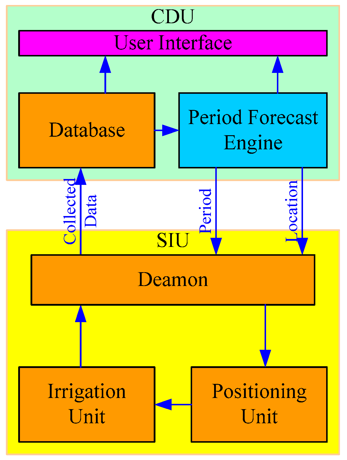
The CAIS had two components, the Core Decision Unit (CDU) and the Sensing and Irrigation Unit (SIU). The CDU analyzed and forecasted the soil moisture. The SIU regularly sampled the soil moisture and controlled the watering system to position the irrigation point. Figure 1 shows the system architecture.

Figure 1.
The system architecture of Constant-moisture Automatic Irrigation System (CAIS). CAIS contains Core Decision Unit (CDU) and Sensing and Irrigation Unit (SIU). The CDU is responsible for analyzing and forecasting the soil moisture and the SIU is responsible for sampling the soil moisture and controls the watering system.
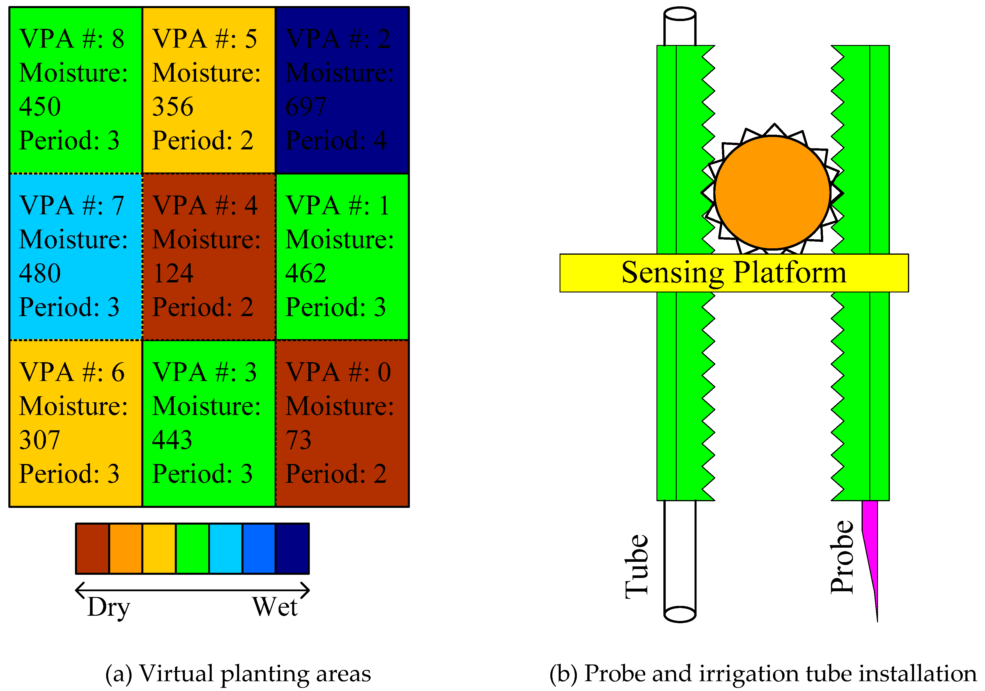
The CDU divided the experimental plot into multiple Virtual Planting Areas (VPAs) shown in Figure 2a. The size of each VPA was similar to the experimental plot used while building the SMF model. The CDU database stored the initial moisture value of each VPA. There was a user interface to display the moisture level of each VPA in different colors. The next irrigation interval of each VPA was also in the CDU. Every time the CAIS executed an irrigation instruction, it also sampled the soil moisture.

Figure 2.
SIU components implementation. (a) The cultivated field is divided into multiple virtual planting areas. CDU applies different irrigation periods for each virtual planting area (VPA). (b) The moisture probing and irrigation components of the CAIS. CAIS uses one motor to control these two components.
The SIU, which was a three-axis device, contained the Positioning Unit (PU), Irrigation Unit (IU), and a daemon to listen to the signal from the CDU. The PU controlled the X-axis and Y-axis to locate the irrigation point of each VPA. The PU used one motor also to control the Z-axis, which installed the moisture sensing probe and the irrigation tube. The IU turned the motor clockwise to examine the soil moisture and counter-clockwise to lower the tube for watering, as shown in Figure 2b. The IU precisely controlled the motor to probe the soil moisture in different depth layers.
2.3.2. Constant Moisture Irrigation Mechanism
To maintain a constant level of soil moisture, the proposed CAIS used a fixed volume of water every time it performed the irrigation but adapted the irrigation interval. To overcome the water siltation caused by the lay of the land, the CAIS set the individual irrigation interval for each VPA. Let HL be the moisture level to be maintained, and xi = (hsc, d*, P, T, ha) be the data just sampled from the ith VPA. The hsc is the current soil moisture sampled by the CAIS. T and ha are the air temperature and humidity, respectively. The d* represents the depth layer of the soil, and P is the previous irrigation interval of this VPA.
Next, the CAIS searched all existing records vj = {Hsj, Tj, Haj, Dj, Pj} in the database which satisfied ha = Haj ± 1, T = Tj, hsc = Hsj, and d* = Dj. These records were classified by the CAIS according to the irrigation interval Pj, and the moisture values of their next records vj+1 so they could be grouped into the corresponding sets {G1, G2, …, Gn}, where n is the number of irrigation intervals. Each set Gw|w=1,2,3…,n, computed the average soil moisture, denoted as (1).
The average moisture value of each set G is . The set Gw with min{|HL-|}|w=1,2,3…,n. is selected, and the corresponding irrigation interval of this set is selected as the next irrigation interval for the ith VPA. All the newly sampled data were added to the database to improve the accuracy.
3. Results
Three specific experiments were conducted to evaluate the SMF model and the CAIS. The first experiment fixed the irrigation interval and applied the SMF model to deduce the probable moisture value for the next CAIS irrigation. This experiment aimed to evaluate the accuracy of the SMF model. The second experiment applied the SMF model and dynamically adapted the irrigation interval to maintain the soil moisture at a constant level for a single irrigation point. The third experiment combined the SMF model and the CAIS to irrigate each VPA. This experiment evaluated whether the CAIS could maintain the soil moisture at a stable level at different locations across the whole experimental plot with multiple irrigation points.
3.1. Evaluation of Soil Sensors
Soil moisture sensors use capacitance to measure the dielectric permittivity of the surrounding medium. The dielectric permittivity is related to the water content of the soil. A soil sensor creates a voltage proportional to the dielectric permittivity. The sensor averages the water content over the entire length of the sensor that is under the surface of the soil.
There were a number of issues with commonly available soil probes, which needed to be addressed. First, soil sensing probes are usually coated with nickel plating, which rusts after 3–4 days when they are left in the soil continuously. Frequently replacing the sensing probe is inconvenient for data collection but also increases the error bias in the detected moisture values because replacing the probe may change the soil density and the position of the monitoring depth layer of soil. Second, the whole surface of the soil sensing probes detects soil moisture in the soil so it is hard to accurately estimate the moisture at a specific depth. Third, the rusted material may introduce heavy metal pollution to the soil, which is not acceptable in organic agriculture. Therefore, we redesigned the probe based on our earlier experiences regarding the material and the exposed parts.
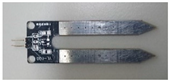
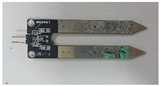
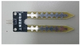
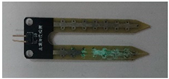
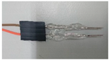
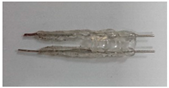
Table 2 shows four kinds of soil sensing probes. The material used in the soil moisture sensors of the first two soil probes is nickel-plated fiberglass. These probes not only rusted quickly but also could not sample soil moisture accurately at a specific depth. Therefore, we initially developed the third probe. The material of the third probe was nickel-plated iron wire, which has nickel-plated fiberglass on the surface with iron inside. It used ethylene vinyl acetate (EVA) to shield the surface and only revealed the tips of the probe. The results showed that the rust-free duration of nickel-plated iron wire was almost double that of the nickel-plated fiberglass. However, when the nickel on the surface of probe rusted, the sampled moisture value changed because the dielectric permittivity was distorted by the iron material. Thus, the alteration to the material produced a sampling error in the moisture data. Therefore, we developed the fourth probe, with a 2 mm diameter copper wire.
Table 2.
Material for designing the soil probe.
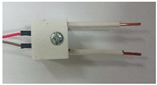
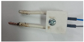
The rust-free duration of the copper wire was about two weeks. To accurately measure soil moisture, only 1 cm of the copper probe needed to be revealed. Figure 3 shows how the probe is used to measure the soil moisture at a depth of 3 cm. This probe only exposed the last 1 cm segment to capture the moisture data while the other 2 cm were covered with plastic. The cap was designed using a 3D printer so the rusted probe can be replaced quickly. Note that the probe in Figure 3 is designed for the general requirements of planting leafy vegetables. Different types of crops will need different probe lengths. This redesigned probe can easily and cheaply prolong the active life of the probe.
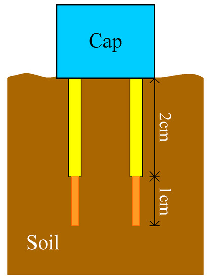
Figure 3.
The sensing probe is redesigned for prolonging the operation time. Frequently replacing the rusted probe increases the error bias on moisture sampling. It is because replacing the probe usually changes the soil density and the position of the monitoring depth layer of soil.
3.2. Experiment 1: Evaluation of SMF Model
The section gives the experimental results for the SMF model deductions and then uses a fixed irrigation interval with the SMF model to deduce the potential moisture value at the next CAIS irrigation.
3.2.1. SMF Model Deduction
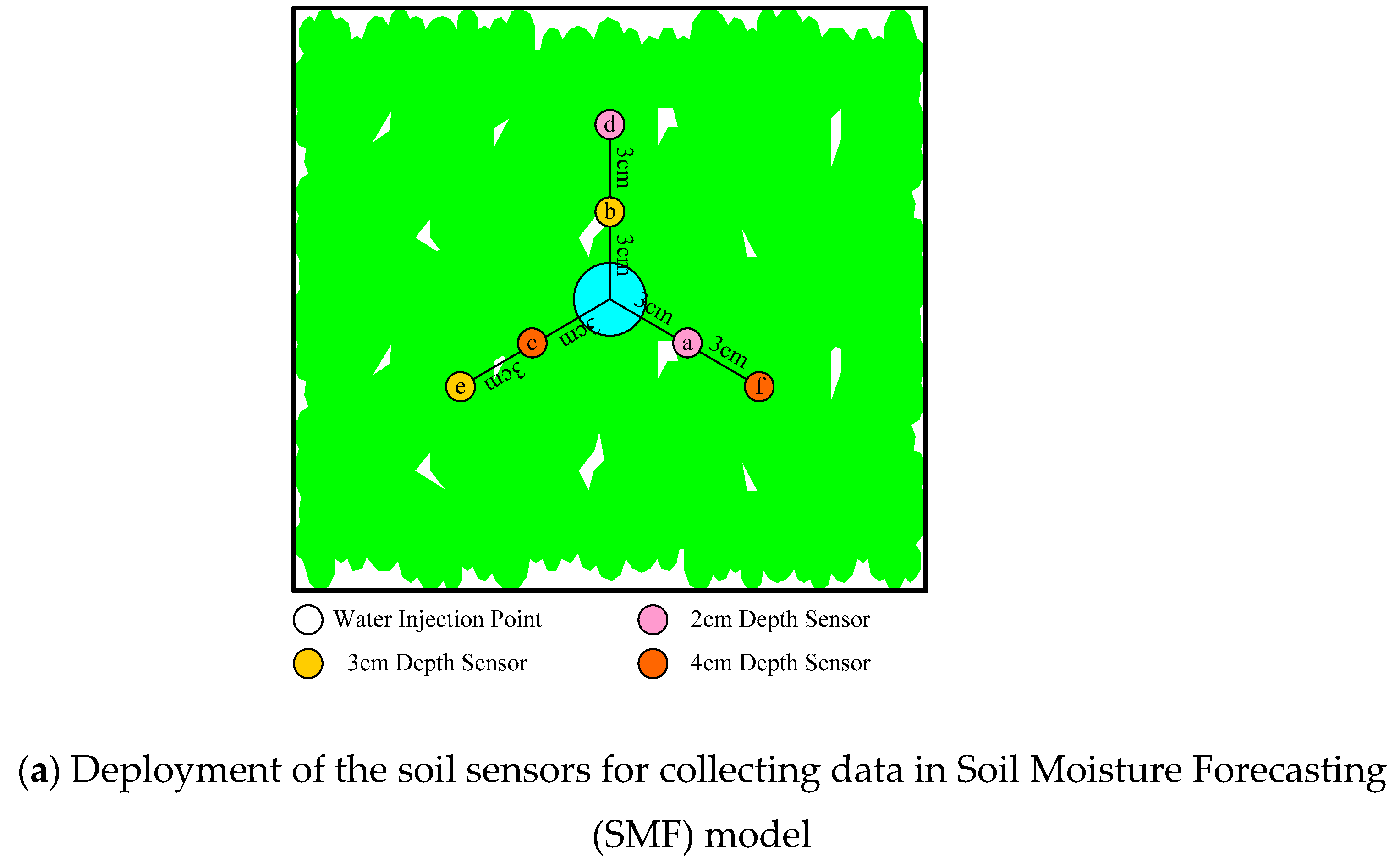
Figure 4a shows the layout of sensors for the SMF model. The probes were placed either 3 cm and 6 cm from the irrigation point to measure water diffusion under the soil. They did not touch the irrigated water directly. They captured soil moisture data at depths of 2 cm, 3 cm, and 4 cm at the sensor locations.

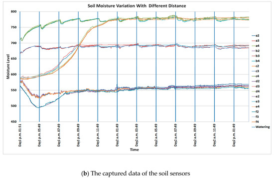
Figure 4.
Data gathering scenario for building the SMF model. The locations {a, b, c} and {d, e, f} are 3 cm and 6 cm to the irrigating point, respectively. The dimension of moisture levels is 0–1023. (a) The soil sensors for collecting data in the SMF model are installed around the watering point with three directions. The distances of the sensor in different directions are the same. (b) The moisture variation of the six installed sensors with different depth layers. The moisture values of the sensors located at 6 cm to the watering point do not have an explicit reaction.
Figure 4b shows the moisture data sampled by the six sensors. In this experiment, 15 mL of irrigation water was applied every 2 h. The sensors were calibrated each time they were plugged into the soil. The comparator chip was an LM393 where the output voltage changed according to the water content in the soil. The output voltage decreased if the soil was wet, and increased if the soil was dry. To provide a more intuitive view of the moisture data, the output values were inversed, so a high value indicated high moisture, and a low value indicated low moisture. Three bottles of soil were prepared for calibration. The first one was dry soil, which was almost a powder. To guarantee that the dry soil contained no water, the soil was placed into a transparent PET (polyethylene terephthalate) bottle and the lid was tightly fastened. The bottle was placed in the sun to check there was no evaporation. The YL-69 voltage value of the dry soil was 0–2. The soil in the second bottle was the original cultivation soil that contained some water. The value captured by the YL-69 ranged from 568 to 570. The bottle was weighed when it was first filled with soil, then water was added if the weight fell. The third bottle mixed dry soil with pure water to completely saturate the soil. The value captured by the sensor was 1020. The sensor calibration first used the second bottle to adjust the output value of YL-69 to range from 568 to 570. Then, the third bottle was used to verify whether the value captured by the sensor ranged from 1020 to 1023. All the sensors sampled the moisture level in the soil every minute. The level of the sampled moisture ranged from 0 (completely dry) to 1023 (completely saturated). The results showed that the moisture values at the 3 cm locations {a, b, c} had a different reaction to the ones at the 6 cm locations {d, e, f} after watering. The moisture values at the locations {d, e, f} did not increase immediately but grew moderately over time. To observe the moisture diffusion under the soil, the experiment used locations 3 cm from the irrigating point to sample the moisture values.
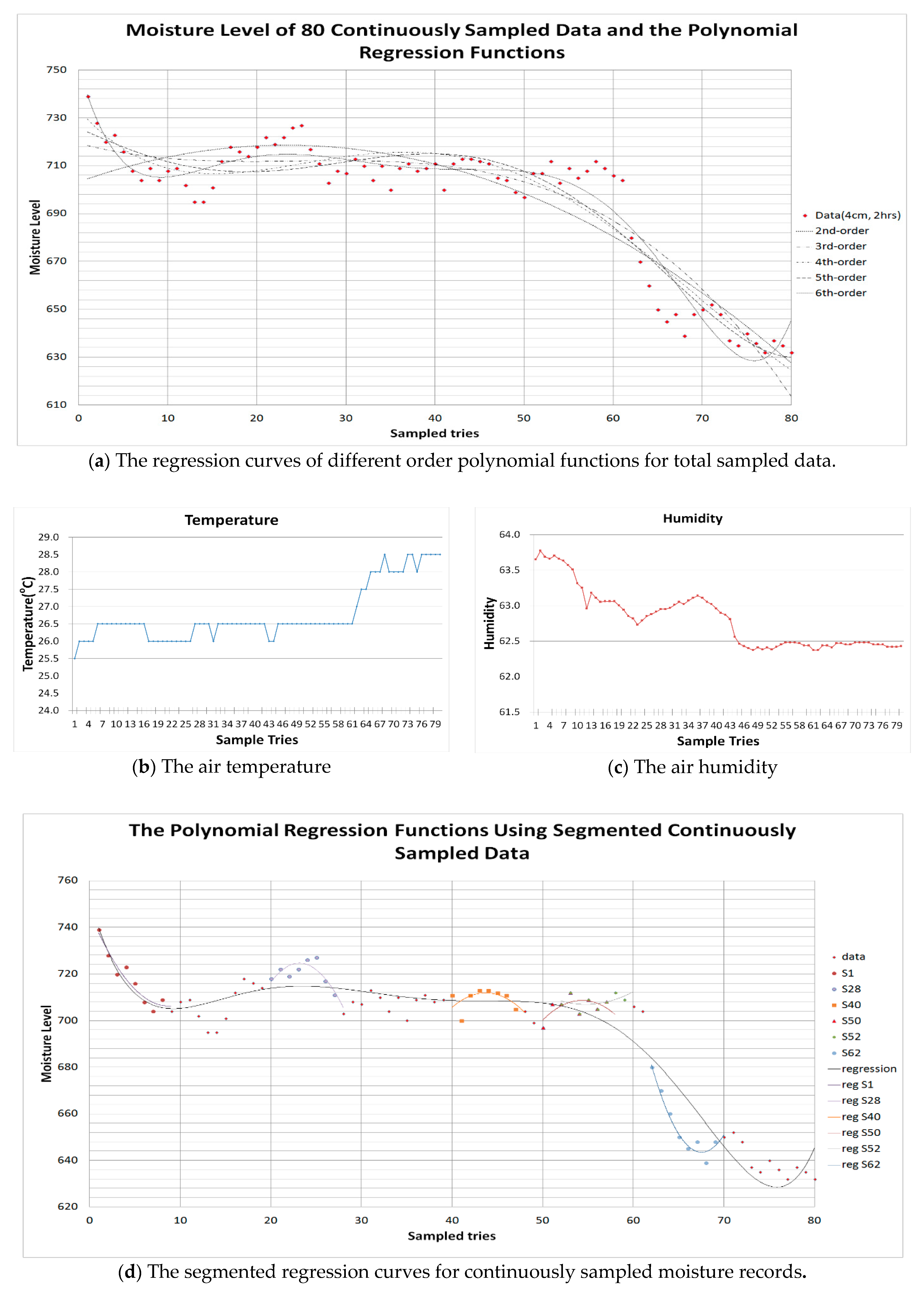
Figure 5a illustrates the moisture data captured by the sensors placed at the 4 cm depth layers of soil and Figure 5b,c show the corresponding values of air temperature and humidity. The irrigation interval in this experiment was 2 h. Sensors sampled the moisture values before irrigation. The total time of this experiment was 160 h. R language was used to compute the regression curve of these sampled values. The results indicated that there was high variability in the data, with many sampled values far from the regression curve. The closest regression function was a sixth-order polynomial function. This test showed that it was difficult to deduce a suitable prediction function from the total sampled moisture dataset because the environmental variability was too high.
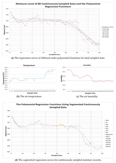
Figure 5.
The regression function of the sampled moisture data. The dimension of moisture level is 0–1023. (a) The regression curves of the 2nd, 3rd, 4th, 5th, and 6th order polynomial functions for total sampled data. (b) The air temperature of this experiment. (c) The air humidity of this experiment. (d) The segmented regression curves. The segment size in this figure is 8 continuously sampled moisture records. Each Sk|k = {1, 28, 40, 50, 52, 62} in this figure is the regression curve using the data from the kth record to the (k + 8)th one. This regression curve is used by the SMF model to forecast the moisture value of the (k + 9)th sampled data.
Figure 5d shows multiple regression curves started from different points. Instead of using the entire sampled dataset, each curve used a small segment of continuously sampled moisture data to deduce the trend function. For example, S1 was the regression curve using the data from the first record to the eighth one. This regression curve was used by the SMF model to forecast the moisture value of the 9th data sample. The S28 used the records from the 28th to the 35th, and the SMF model used this regression curve to forecast the moisture of the 36th data sample. The results were closer to the observed moisture data samples than the regression curve for the whole dataset.
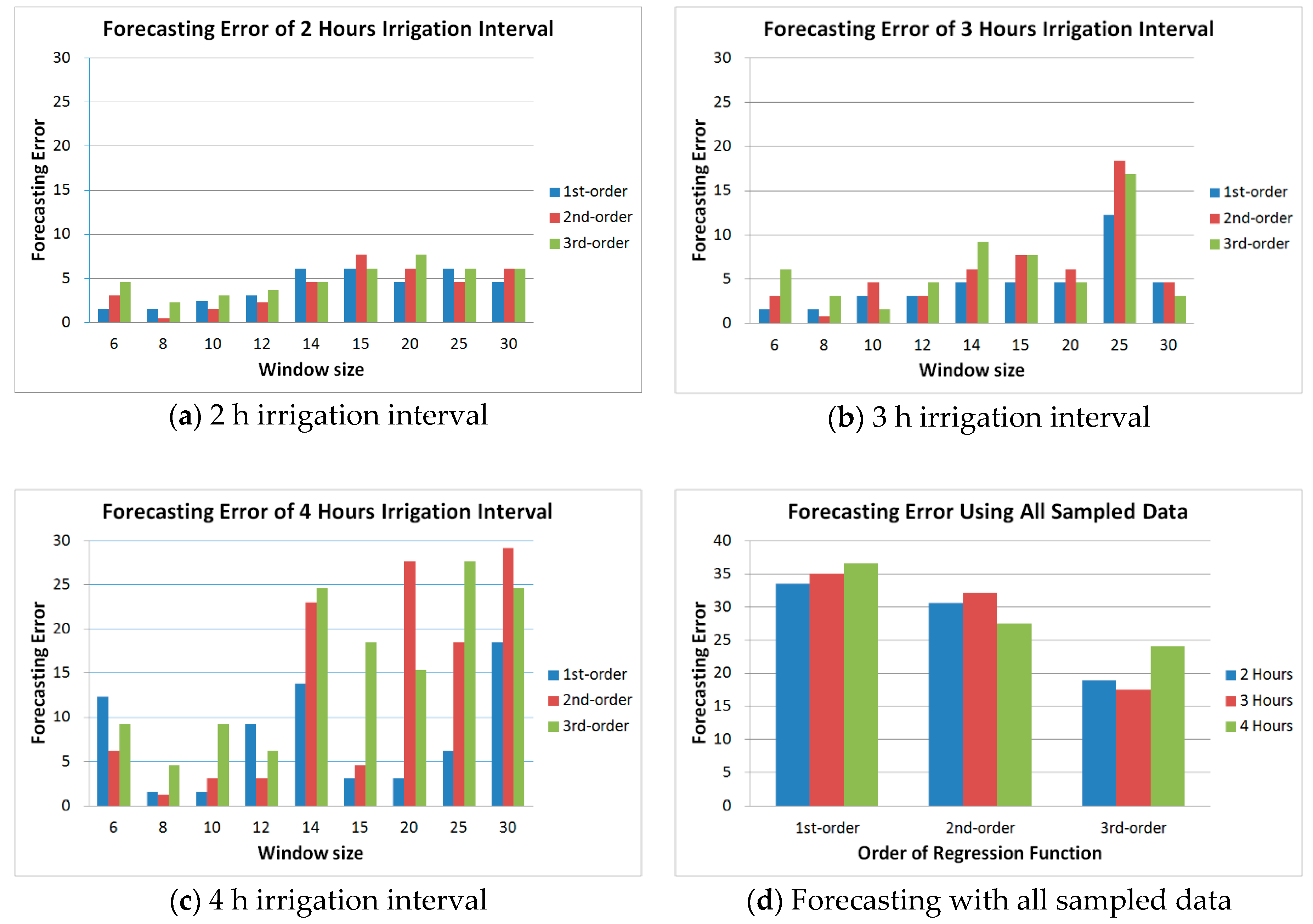
The size of continuously sampled moisture records in a segment is known as the extract window, denoted as W. Our objective was to determine a suitable W size to minimize the distance between the sampled data and the regression curve. The evaluated sizes of W included 6, 8, 10, 12, 14, 15, 20, 25, and 30. Figure 6 shows the results of the 1st, 2nd, and 3rd order polynomial regression functions with 2, 3, and 4 h irrigation intervals. Here, the forecasting error is defined as (Mf–Mr)/Mmax. Mf is the forecasted moisture level using the regression function of the segmented sampled data, Mr is the real moisture value sampled by the sensors, and Mmax is the maximal scale at which the sensors sample the moisture.
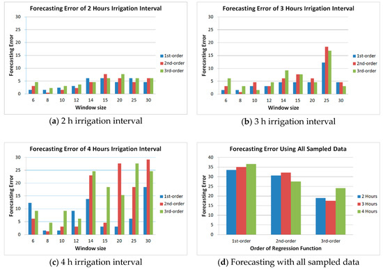
Figure 6.
The forecasting accuracy of different window sizes. The sensors placed at the 3 cm depth layers of soil. The forecasting error is estimated in moisture levels. The dimension of moisture level is 0–1023. (a) The results of the forecasting error by using the 2 h irrigation interval. (b) The results of 3 h irrigation interval. (c) The results of 4 h irrigation interval. (d) The results of using all the sampled data.
Figure 6a–c shows the forecasting errors for different irrigation intervals. Figure 6d shows the non-segmented moisture records for comparison. The forecasting error evaluates the difference between the real capture voltage value of the YL-69 sensor and the deduced value from the SMF model. Figure 6a shows the forecasting errors for a 2 h irrigation interval from sensors placed at the 3 cm soil depth. The results indicated that the forecasting error was smaller if the applied window sizes were 8, 10, or 12; their average forecasting errors of the moisture level were 1.5–2.3, 1.5–3.1, and 2.3–3.7, respectively.
Figure 6b shows the forecasting errors when the experiment used a 3 h irrigation interval. The lowest average forecasting errors on the moisture level were with window sizes 6 and 8 (1.5–6.1 and 0.8–3.1, respectively). Figure 6c shows the average errors of the 4 h irrigation interval. The errors in window sizes 8, 10, and 12 were lower than the others, at 1.5–4.6, 1.5–9.2, and 3.1–9.2, respectively. The experimental results suggest that a 2nd-order regression function with a window size set to 8 gave the best forecasting accuracy. When all sampled data were used as the extract window, the forecasting errors on the moisture level in every irrigation interval were 17.5–36.6 shown as Figure 6d. This level of error cannot predict the true variation of soil moisture.
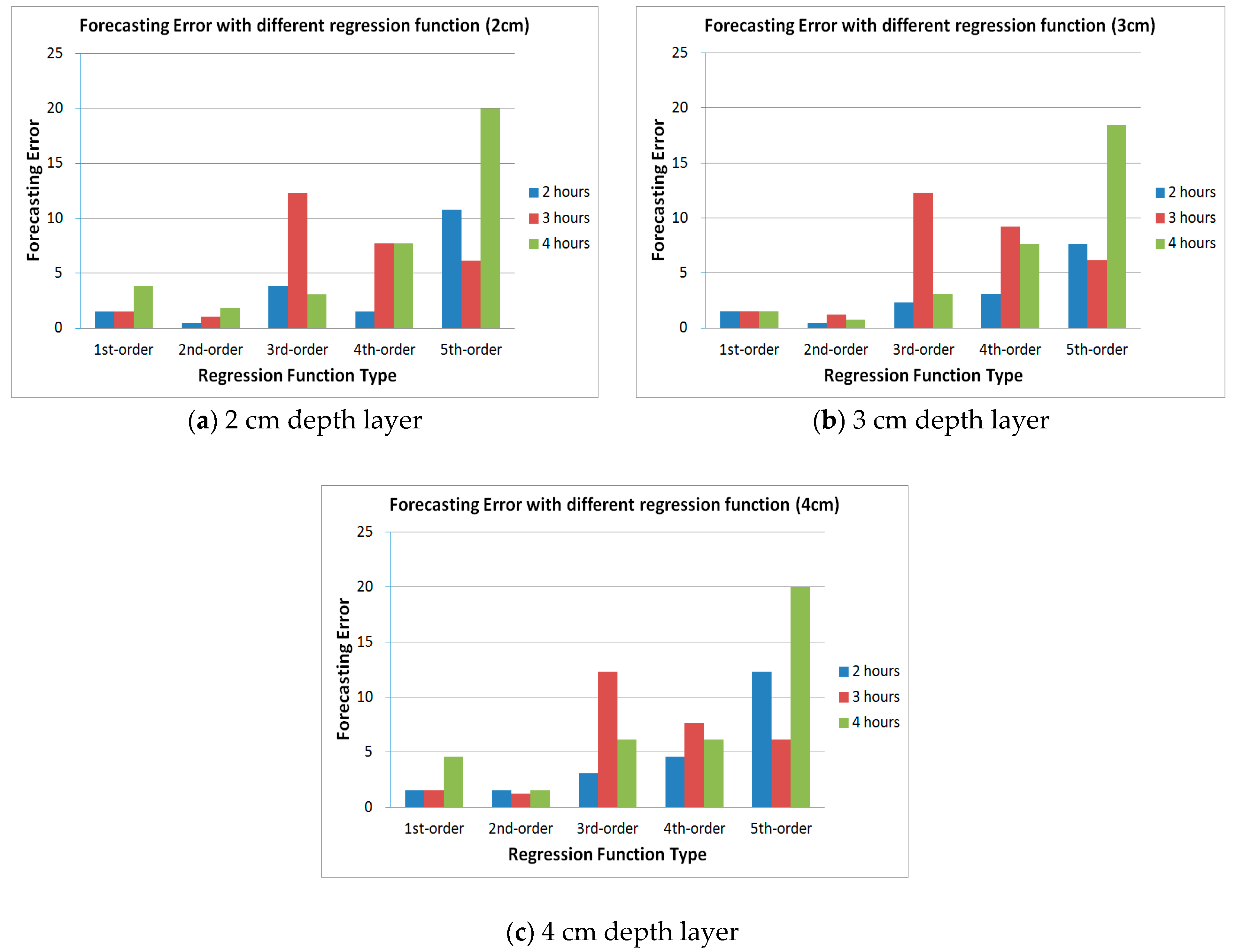
The next experiment verified higher-order polynomial regression functions to discover which were best at forecasting. Figure 7a–c shows the forecasting errors for moisture at 2 cm, 3 cm, and 4 cm depths. For the data in every soil depth layer, this experiment used the 1st, 2nd, 3rd, 4th, and 5th-order regression functions to forecast moisture. The results indicated that forecasting errors grew with the order of function. The 2nd-order polynomial function had the smallest error on average. These results confirmed that a 2nd-order regression function with window size set to 8 was suitable for the SMF model.
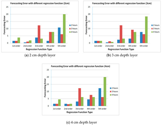
Figure 7.
The forecasting errors of different order polynomial functions. The 1st-order to 5th-order polynomial regression function with different irrigation intervals are evaluated. The forecasting error is calculated by moisture level, which is ranged from 0 to 1023. (a) the results of the sensors placed at the 2 cm depth layer of soil. (b) the results of the sensors at the 3 cm depth layer of soil. (c) the results of the sensors at the 4 cm depth layer of soil.
3.2.2. Experimental Results
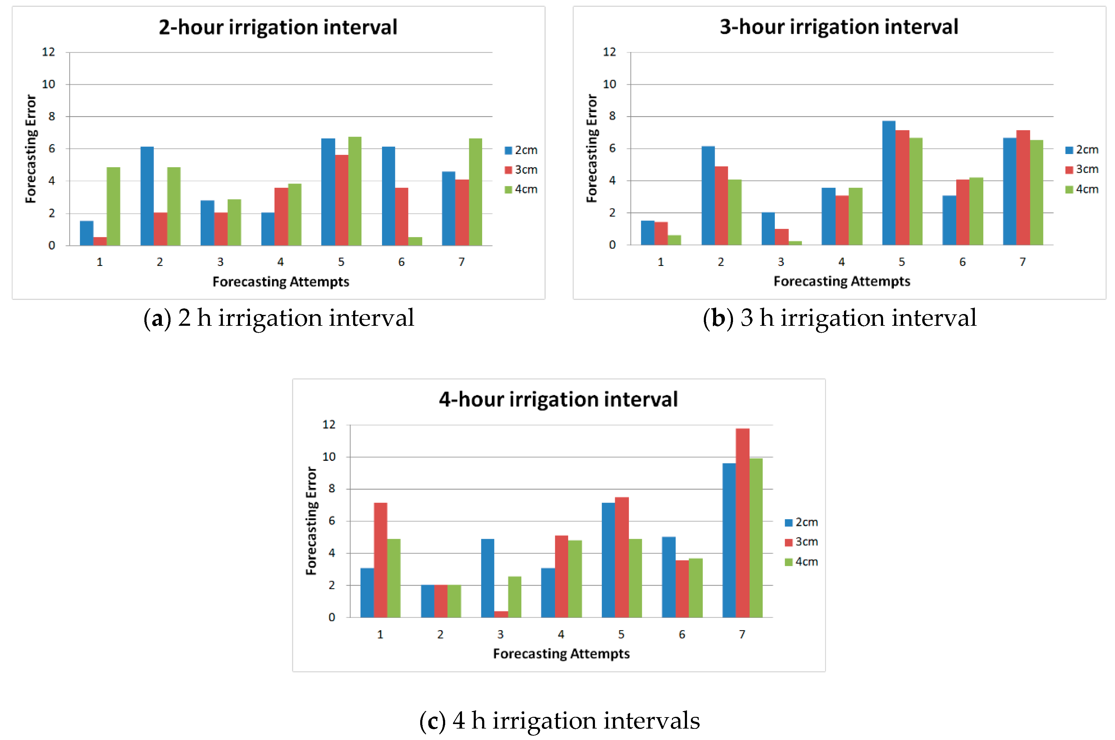
In this experiment, the experimental medium was potting soil made from mushroom wood chips and coconut fibers. The total size of the experimental plot was 120 cm × 90 cm and the height was 6 cm. The sensors were placed at VPA#4. The area of each VPA was a 39 cm × 28 cm rectangle. The watering volume was 15 mL each time the SMF performed the irrigation task. The moisture forecasting in this experiment was executed seven consecutive times, and each forecasting result was compared with the observed soil moisture values. The objective was to verify the error of the SMF model.
Figure 8a–c shows the forecasting errors when the SMF applied the 2, 3, and 4 h irrigation intervals. In the case of the 2 h irrigation interval, the error on the moisture level was no more than 7. The 3 h irrigation interval was relatively similar, with an error of no more than 8. The maximum error was in the 4 h irrigation interval, at 11.8, with an average forecasting error of less than 9.9 in this interval. These results show that the forecasting error of the SMF model was no more than 12 moisture levels out of 1024 possible levels.
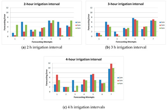
Figure 8.
The continuous forecasting errors of the SMF model with the real sample results. The forecasting error is evaluated by moisture level, which is ranged from 0 to 1023. (a) The forecasting errors of 2 h irrigation interval. (b) The forecasting errors of 3 h irrigation interval. (c) The forecasting errors of 4 h irrigation interval.
3.3. Experiment 2: Evaluation of the CAIS with Single Irrigation Point
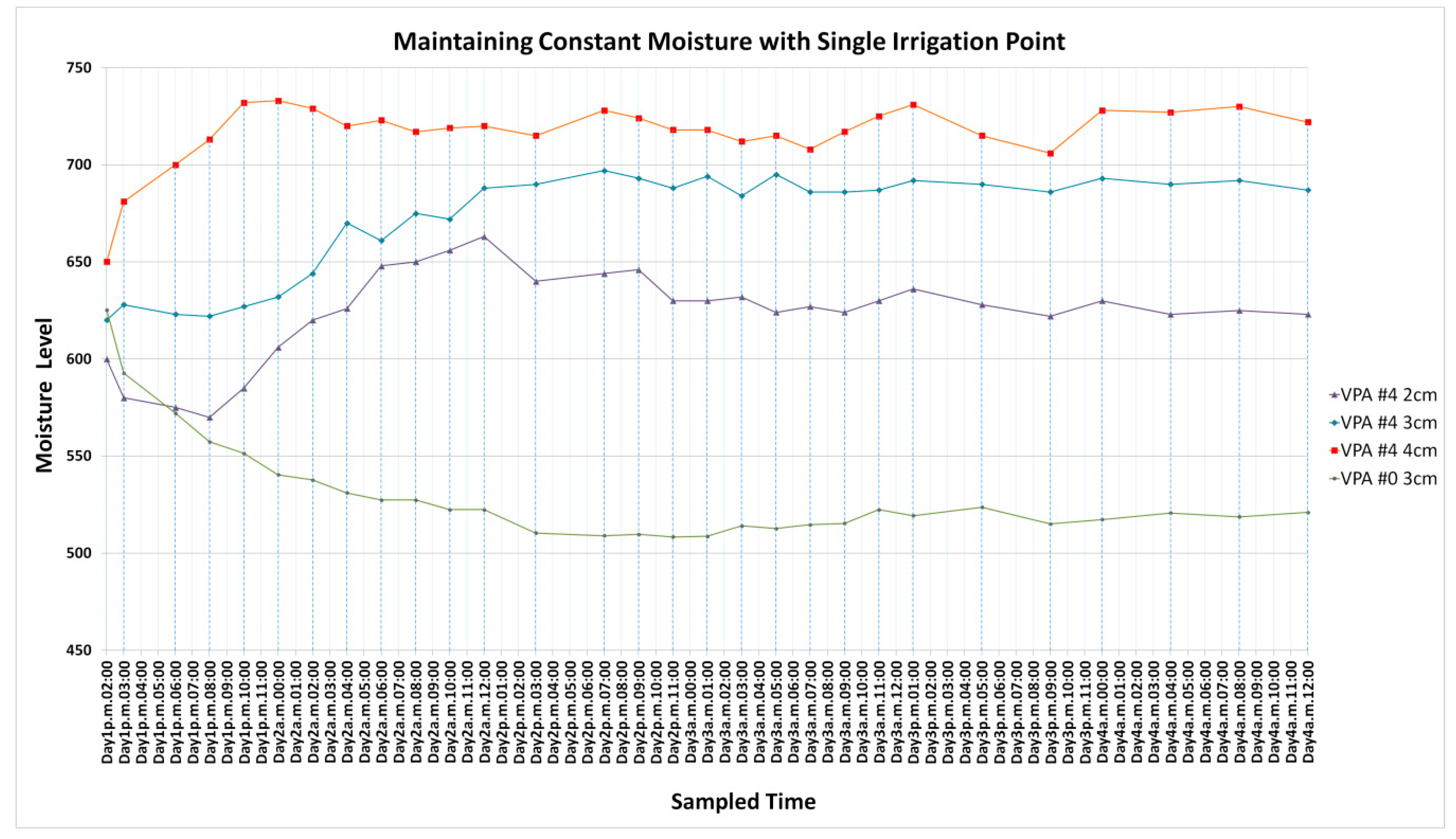
The aim of this experiment was to retain the moisture of the 3 cm depth layer soil at level 690. The parameters of air humidity and the air temperature were the same as those used to build the SMF model. The sensor captured the moisture value from VPA#4 of the experimental plot. The vertical dashed lines in Figure 9 indicate the time when the CAIS performed the irrigation task. The experiment started at p.m. 02:00 on Day 1. The initial soil moisture sampled by the sensors at 2 cm, 3 cm, and 4 cm depth layers, denoted as S2, S3, and S4, was 601, 624, and 649, respectively. The irrigation intervals for selection were 2 h, 3 h, and 4 h.
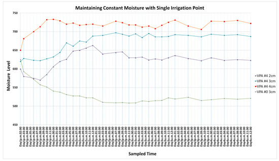
Figure 9.
The constant moisture experiment with a single irrigation point. The moisture levels of VPA#4 with different depth layers of soil are sampled. The VPA#0 3 cm, which is the neighboring VPA, is also evaluated. The moisture level is ranged from 0 to 1023.
The first irrigation task was at p.m. 03:00 on Day 1. At this time, the CAIS determined the next irrigation interval was 3 h based on the data from the SMF model. The next irrigation time was at p.m. 06:00 on Day 1. At this time, the moisture level of S3 was 625, which was well below the desired 690 level and the CAIS shortened the irrigation interval to 2 h. From then on, the CAIS actively increased the moisture level by maintaining the 2 h irrigation interval until p.m. 12:00 on Day 2.
Figure 9 also shows the moisture level of the 3 cm depth layer in VPA#0, denoted as VPA#0 3 cm. The moisture level fell continuously and became stable after p.m. 03:00 on Day 2. This status continued until a.m. 01:00 on Day 3 and then grew moderately until the end of the experiment. The location of VPA#0 was far from the irrigation point and its moisture level was much lower than the required level 690. The average error bias of the moisture level was higher than 150. As the water continuously evaporated from the media and VPA#0 was not directly resupplied by irrigation water, the moisture levels fell. The increasing trend of the moisture levels after a.m. 11:00 on Day 3 came from water under the soil gradually infiltrating from VPA#4. However, the speed of evaporation was higher than that of infiltration. Thus, the VPA#0 moisture level maintained a relatively stable state with slight growth.
3.4. Experiment 3: Evaluation of the CAIS with Multiple Irrigation Points
The previous experiment demonstrated that the CAIS could retain the soil moisture near the irrigation point at a constant level. This experiment used the CAIS at multiple adjacent irrigation points to maintain the soil moisture level of the whole experimental plot at a specific level. The experimental plot has night irrigation areas similar to Figure 2a. The setup of the experimental parameters was the same as Section 3.2. To guarantee that the soil moisture in the experimental plot could evaporate and diffuse completely, the CAIS performed regular irrigation every 3 h for 24 h before the experiment began.
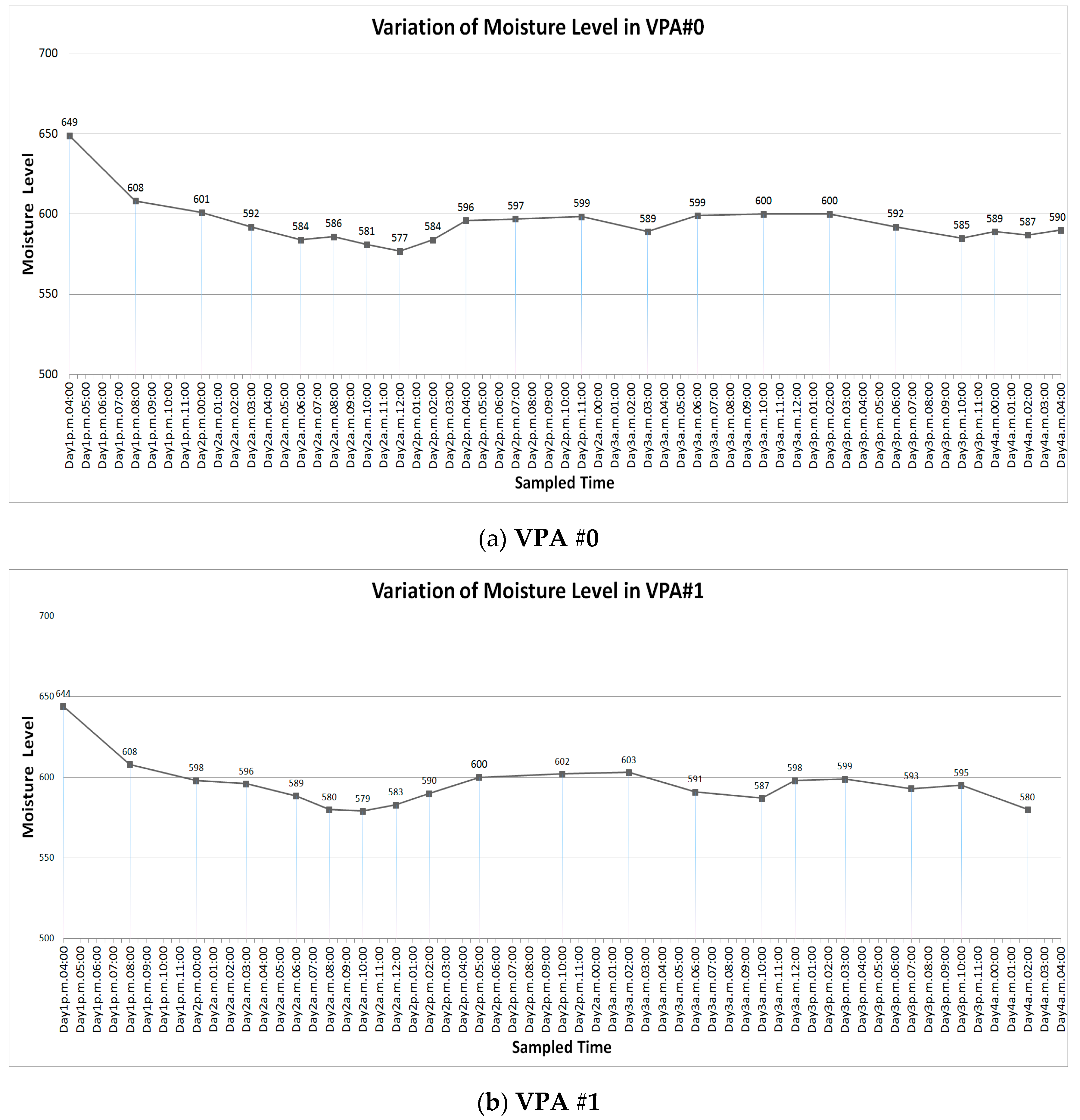
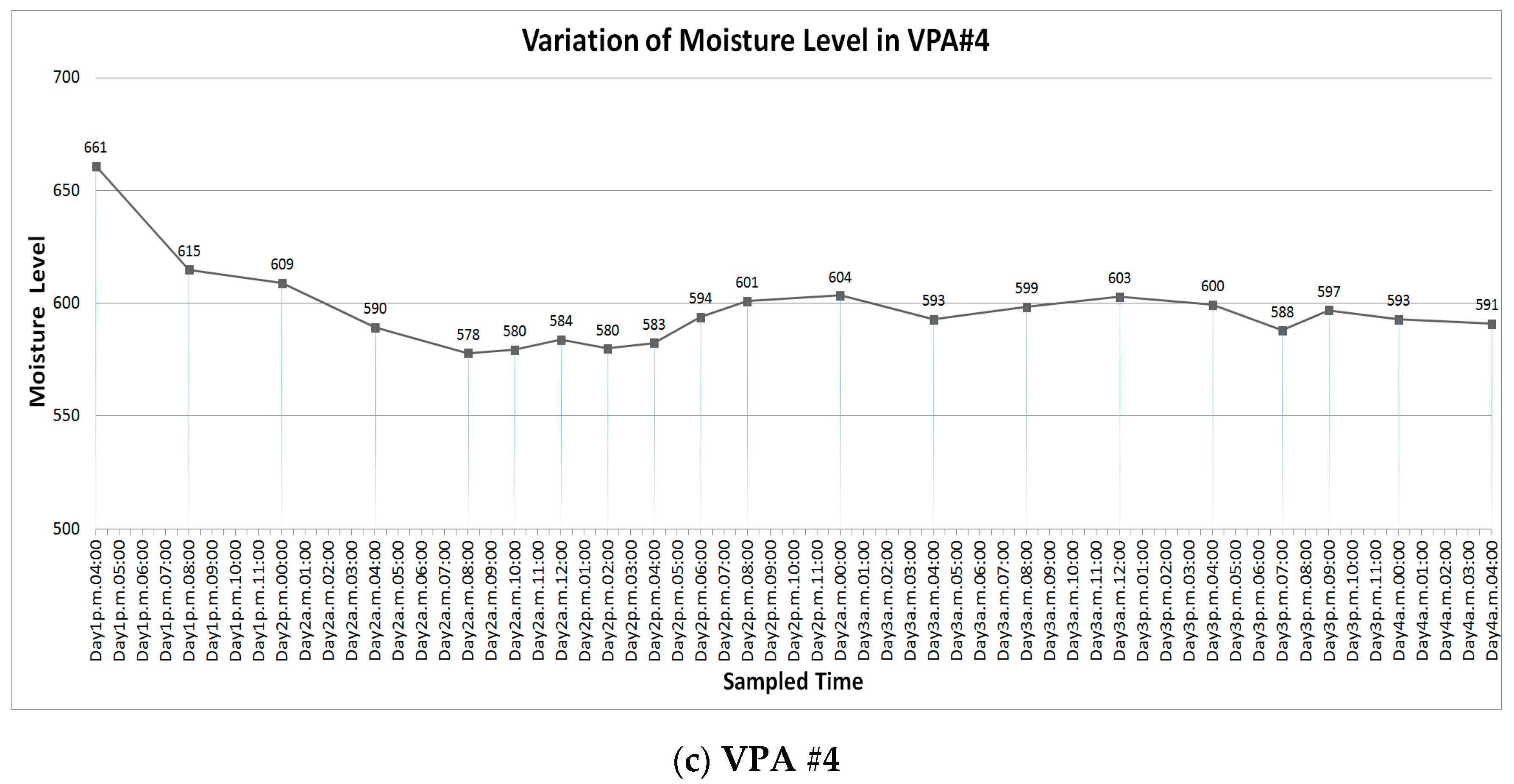
Figure 10a–c shows the moisture levels at points VPA#0, VPA#1, and VPA#4. The selectable irrigation intervals were 2, 3, and 4 h. The CAIS started the first irrigation at p.m. 04:00 on Day 1. The objective was to maintain the moisture level at 590 for all 3 cm soil depths in these three areas. Note that instead of placing the probe in the soil continuously, the soil sensor used the CAIS platform described in Section 2.3.1 to probe each VPA every 30 min. Intermittent probing can prevent rusted probes from introducing heavy metal pollution to the soil. Each probe lasted for one minute and sampled the soil moisture every second. The moisture value from the probe was averaged for all 60 data samples.
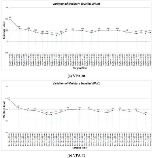
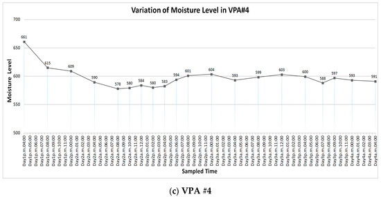
Figure 10.
The moisture levels of the sensors at the 3 cm depth layer in different VPA. The moisture level is ranged from 0 to 1023. (a) the moisture level of the VPA#0. This VPA is located at the corner of the experimental plot. Similar VPAs are VPA#2, VPA#6, and VPA#8. (b) the moisture level of the VPA#1. Similar VPAs are VPA#3, VPA#5, and VPA#7. (c) the moisture level of the VPA#4, which is at the center location of the experimental plot.
The first sampled moisture levels of these three VPAs were 649, 644, and 661. These levels were higher than the required moisture level 590. The CAIS applied two 4 h irrigation intervals for all the VPAs to reduce their soil moisture levels. By Day 2 a.m. 00:00, their moisture levels were 598, 601, and 609. The CAIS adapted the irrigation interval of VPA#0 and #1 to 3 h. Their moisture levels continuously decreased until Day 2 a.m. 06:00. At Day 2 a.m. 06:00, the moisture levels of VPA#0 and VPA#1 were 584 and 589. The CAIS changed the irrigation interval to 2 h to raise their moisture levels until Day 2 p.m. 02:00. Figure 10a–c shows the results.
In Figure 10a, the CAIS continuously used the 2 h irrigation interval to raise the moisture level of VPA#0 until Day 2 p.m. 04:00, when the moisture level reached 596. The CAIS then adjusted the irrigation interval to 3 h and 4 h to suppress the rising moisture level. The moisture level at Day 3 a.m. 03:00 was 589 so the CAIS changed the irrigation interval to 3 h. However, the moisture level was still close to 600 on Day 3 a.m. 06:00. The CAIS applied a 4 h irrigation interval to alleviate the moisture level until Day 3 p.m. 10:00. The moisture level at Day 3 p.m. 10:00 decreased to 585, and the CAIS used the 2 h irrigation interval until Day 4 a.m. 04:00.
In Figure 10b, the moisture level at Day 2 p.m. 02:00 was 590. The CAIS used the 3 h irrigation interval to moderate the increasing moisture level of VPA#1. However, the moisture level did not explicitly decrease even though the CAIS continuously applied the 3- and 4 h irrigation intervals until Day 3 a.m. 10:00. This phenomenon arose from the different density of the planting medium. However, by Day 4 a.m. 02:00, the moisture level (580) had fallen below the required level of 590.
VPA#4, which was located in the center of the experimental plot, was influenced by the neighboring VPAs. Initially, its moisture level was higher than 590, and the CAIS applied the 4 h irrigation interval until Day 2 a.m. 08:00 shown as Figure 10c. By Day 2 a.m. 08:00, the moisture level had fallen to 578. The CAIS then applied 2 h irrigation to raise the level until Day 2 p.m. 08:00. The moisture level on Day 2 p.m. 08:00 was 601. The CAIS switched to the 4 h irrigation interval to lower the moisture level until Day 3 p.m. 07:00. The moisture level at this time was 588. The next adjustment raised the moisture level and the 4 h irrigation interval was continuously applied until the end of the experiment.
The duration over which the CAIS adjusted the moisture levels of these three areas to 590 was about 24 h, as shown by the experimental results between Day 2 p.m. 04:00 and Day 2 p.m. 06:00 in Figure 10a–c. The average sampled moisture levels computed from Day 2 p.m. 04:00 to the end of the experiment on Day 4 a.m. 04:00 for these three areas were 595, 594, and 595, respectively. The average error bias was ±5 moisture levels. The results proved that the CAIS maintained a constant moisture level by changing the irrigation interval of each VPA. Dividing the experimental plot into multiple areas efficiently reduced the impacts of soil density on soil moisture. The water was evenly distributed and retained a balanced moisture value over the whole experimental plot.
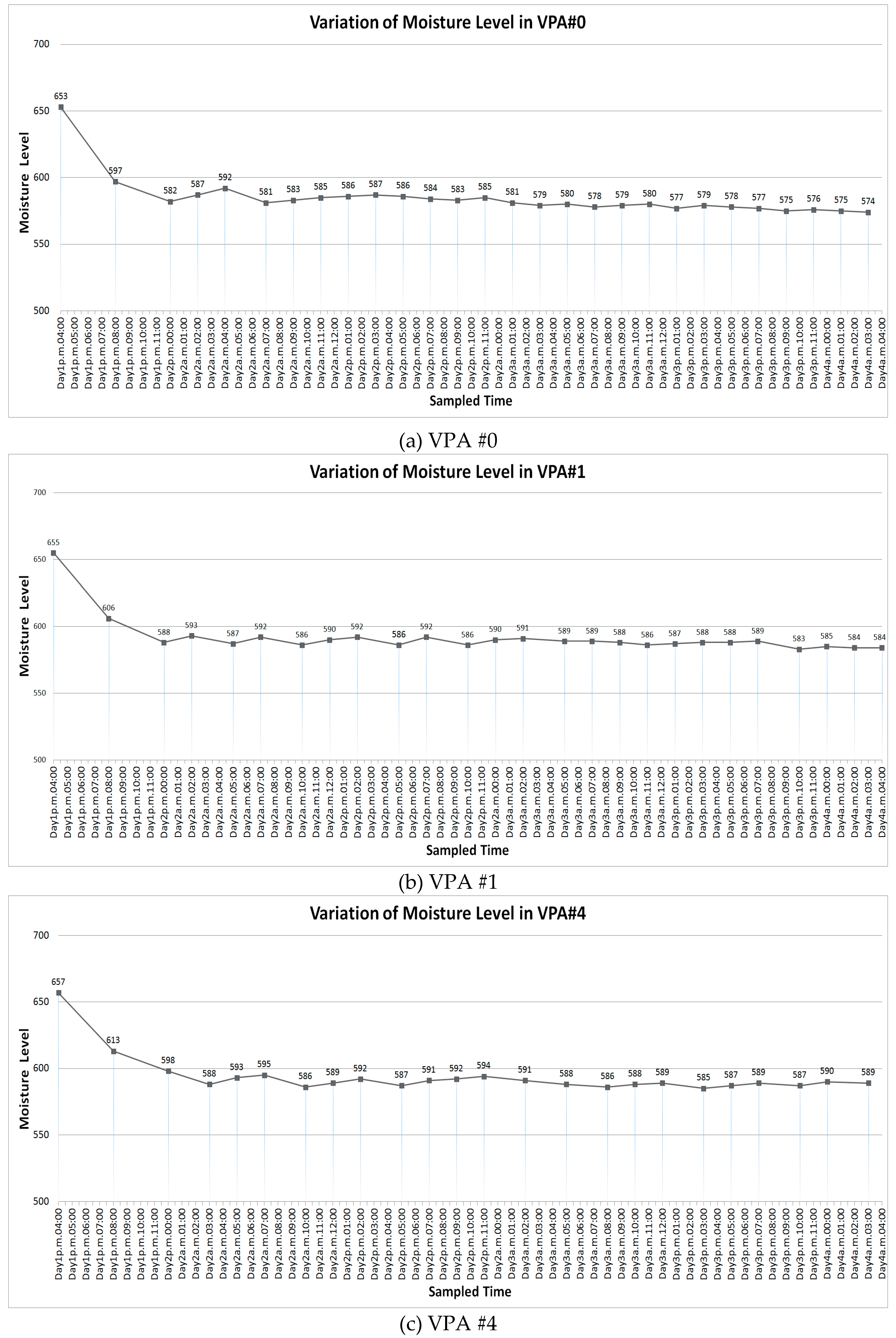
An experiment with high air temperature, which is 30 °C–34 °C, is evaluated. The experimental platform is placed under the air conditioner vent. The surrounding humidity of this experiment is 58–68%. Figure 11a–c is the moisture levels of VPA#0, VPA#1, and VPA#4, respectively. The selectable irrigation intervals are also 2, 3, and 4 h. We also started the first irrigation on Day1 p.m. 04:00. The object is also to maintain the moisture level at 590 for all 3 cm depth layer of soil of these three areas.
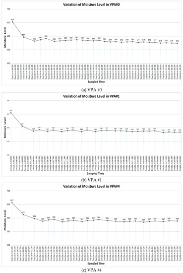
Figure 11.
The moisture levels of the sensors at the 3 cm depth layer in different VPA with high air temperature (30 °C–34 °C). The moisture level is ranged from 0 to 1023. (a) the moisture level of the VPA#0. This VPA is located at the corner of the experimental plot. Similar VPAs are VPA#2, VPA#6, and VPA#8. (b) the moisture level of the VPA#1. Similar VPAs are VPA#3, VPA#5, and VPA#7. (c) the moisture level of the VPA#4, which is at the center location of the experimental plot.
The first sampled moisture levels of these three VPAs were 653, 655, and 657. CAIS applied the 4 h irrigation interval for all of these VPAs to reduce their soil moisture levels. Their moisture levels changed to 582, 588, and 598. In Figure 11a, CAIS adapted the irrigation interval of VPA#0 to 2 h At Day 2 a.m. 00:00, and the moisture level of VPA#0 continuously increases. At Day 2 04:00, CAIS changed the interval to 3 h because the increasing rate of the moisture level is too fast. At Day 2 a.m. 07:00, the moisture level reduced to 581. CAIS changed the interval to 2 h and the irrigation interval did not alter until the end of this experiment. The high air temperature increases the evaporating rate that the planting media at VPA#0 cannot hold water. Thus, the distance between the sampled moisture level and the required one gradually draws apart.
For the VPA#1, CAIS adapted the irrigation interval 2 h and 3 h alternatively within the interval Day 2 a.m. 00:00 and Day 3 a.m. 05:00 shown as Figure 11b. The high evaporating rate caused by the high air temperature also influences the planting media at VPA#1. Thus, the 2 h irrigation interval is almost applied to the end of this experiment after Day 3 a.m. 05:00 at VPA#1. Because VPA#1 has one more neighboring VPA than VPA#0, it can absorb the contained water from neighboring fields to balance the soil moisture.
VPA#4, which locates at the central position of the experimental plot, has its moisture level close to the required 590. More than one sampled value of the moisture level is higher than 590 before Day 3 a.m. 05:00. It has a shorter moisture level distance between the sampled value and the required one. More neighboring VPA makes it easier to balance the soil moisture than others.
4. Discussion
In the first experiment, the SMF model continuously forecasts the next seven sampled moisture levels and compared them with the practice sampled moisture levels. The measuring scale of the sensing components in this article is 0 to 1023. The forecasting error is less than 1.2% measuring scale. Using a small segment of the continuously sampled moisture records can help the SMF closely fit the soil moisture variation caused by environmental factors. In this experiment, by applying the moving average in statistics, the forecasting error on the moisture levels is 18 to 32. The experimental results are not better than the SMF model. From the results of Figure 8, the forecasting errors by using long irrigation intervals seem higher than that of the short ones. Forecasting the moisture levels in long irrigation intervals will suffer more influences from the environmental factors. So, the results are worse than the short irrigation intervals. In this work, the SMF model uses fix segment size of continuously sampled records to forecast the moisture. If the segment size can be dynamically adjusted by referring to the environmental factors, the results must be improved further. This will be the next research topic.
In the second experiment, the CAIS watered the experimental plot from one point. This experiment just evaluated the 3 cm depth layer soil near the watering location. In this experiment, CAIS spends about 24 h to steady the soil moisture at the target level. The moisture levels, which are detected by the sensors placed at 2 cm, 3 cm, and 4 cm depth layer in VPA#4, increase and then become stable after CAIS adapts irrigation interval. The fluctuations of the moisture levels captured by the sensors placed at 2 cm and 4 cm depth layer of soil are larger than the sensors placed at the 3 cm depth layer because the irrigation interval adjustment is according to the 3 cm depth layer sensor. The moisture levels at different depth layers of soil also influence the moisture levels of 3 cm ones. For the neighboring VPA#0, the soil moisture does not retain at the target level explicitly. However, the containing water in the soil will also influence the moisture level of the VPA#4. Thus, the experiment with multiple irrigation points is necessary for proving the moisture-retaining ability of the CAIS.
CAIS can only retain the constant soil moisture at a small area in the scenario that the amount of water is only 15 mL in each watering. Thus, the next experiment evaluates the case with multiple irrigation points. The testbed is divided into nine VPAs shown in Figure 2a. The moisture level of VPA#0, VPA#1, and VPA#4 are captured. The object is to maintain the moisture level at 590 for all 3 cm depth layer of soil. In Figure 10, each of these three VPAs uses different irrigation intervals to keep the soil moisture staying at the target level. The moisture levels in each VPA become steady after about 24 h. The time for the moisture becoming steady is on Day2 20:00. In these three VPAs, most of the applied irrigation intervals are 3 h and 4 h after the time Day 2 20:00. Using multiple irrigation points produces more water to the experimental plot than using a single irrigation point. Therefore, CAIS prolongs the irrigation interval for adjusting the moisture level to retain the moisture at the target level. The results also indicate that dividing the experimental plot into multiple areas can efficiently reduce the impacts of soil density on soil moisture. The irrigated water can be evenly distributed to the whole experimental plot. Currently, CAIS only consider the moisture at a specific soil depth layer. If the irrigation interval selection can consider different depth layers of soil, the moisture level must be more stable, and this is the future work of the CAIS.
Table 3 gives the comparison results of the proposed CAIS with the existing products. The watering area of the Brass Impact Sprinkler [31] is about 78 m2. It is triggered by the water pressure. If it integrates with the Watering Timer [32], the auto irrigation can be active. The watering volume is not precisely controlled. FarmBot [33] is the intelligent irrigation product that most likely to the proposed CAIS. FarmBot can water, seed, and sensing automatically over a predefined experimental plot. Users can use the website to adjust the planting parameters. The scale of this product is fixed. All of the existing products do not have the ability to maintain the constant moisture and the learning mechanism.
Table 3.
Operational characteristics of CAIS vs. other existing products or components.
5. Conclusions
In this paper, we presented the development of a dynamical Constant-moisture Automatic Irrigation System in conjunction with a Soil Moisture Forecasting Model. We used redesigned sensing probes in the model to prolong the durability of each probe and to reduce the inaccuracy of data caused by replacing the sensing probe. Many experiments were performed to infer the optimal continuous sampling window for the moisture forecasting function. This approach provided useful detail on the spatial variability of water demand. The moisture forecasting accuracy of the proposed SMF model is higher than 98%. The proposed Constant-moisture Automatic Irrigation System, named CAIS, focuses on developing a low-cost system for the greenhouse system, a small experimental plot, or the scenario for high economic value crops. CAIS uses a three-axis platform with the SMF model to keeps the soil moisture at a constant level. CAIS probes the moisture data on demand to prevent heavy metal pollution on the soil and adapts the irrigation intervals of multiple irrigation areas to hold the soil moisture of the whole cultivated plot at the required level. The CAIS can stabilize the moisture level within ±5 points in 24 h in either normal or high atmospheric temperature environments. The experimental results demonstrate that CAIS can provide a stable moisture level in the growing media.
Author Contributions
Conceptualization, S.-C.H.; methodology, S.-C.H.; software, Y.-Z.L.; validation, S.-C.H. and Y.-Z.L.; formal analysis, S.-C.H.; investigation, S.-C.H.; resources, Y.-Z.L.; data curation, Y.-Z.L; writing—original draft preparation, S.-C.H.; writing—review and editing, S.-C.H.; visualization, S.-C.H. All authors have read and agreed to the published version of the manuscript.
Funding
The APC of this research was funded by Ministry of Science and Technology (MOST), Taiwan, grant number MOST109-2637-E-150-004.
Conflicts of Interest
The authors declare no conflict of interest.
References
- Gutiérrez, J.; Villa-Medina, J.F.; Nieto-Garibay, A.; Porta-Gándara, M.Á. Automated Irrigation System Using a Wireless Sensor Network and GPRS Module. IEEE Trans. Instrum. Meas. 2014, 63, 166–176. [Google Scholar] [CrossRef]
- Kim, Y.; Evans, R.G.; Iversen, W.M. Remote Sensing and Control of an Irrigation System Using a Distributed Wireless Sensor Network. IEEE Trans. Instrum. Meas. 2008, 57, 1379–1387. [Google Scholar]
- Rao, R.N.; Sridhar, B. IoT based smart crop-field monitoring and automation irrigation system. In Proceedings of the International Conference on Inventive Systems and Control (ICISC), Coimbatore, India, 19–20 January 2018; IEEE: Piscataway, NJ, USA, 2018; pp. 478–483. [Google Scholar]
- Ramachandran, V.; Ramalakshmi, R.; Srinivasan, S. An Automated Irrigation System for Smart Agriculture Using the Internet of Things. In Proceedings of the International Conference on Control, Automation, Robotics and Vision (ICARCV), Singapore, 18–21 November 2018; pp. 210–215. [Google Scholar]
- Silva, M.; Junior, L.H.; Carneiro, E.J.P.; de Matos, K.M.; Anacilia, J.P.; de Vieira, M.C.; da Silva Barreto, A. Raimundo. Tellus—Greenhouse Irrigation Automation System. In Proceedings of the IEEE Symposium on Computers and Communications (ISCC), Natal, Brazil, 25–28 June 2018; pp. 01239–01242. [Google Scholar]
- Muthukumar, S.; Karthikeyan, K.; Ranjithkumar, G.; Kavin, R. A Cost Effective System for Auto Irrigation, Soilmonitoring and Control. In Proceedings of the International Conference on Soft-computing and Network Security (ICSNS), Coimbatore, India, 14–16 February 2018; pp. 1–7. [Google Scholar]
- Li, M.; Tian, L.; Chen, Z.; Wu, X.; Wang, Y. A kind of imitated environment system for plant growth based on LED light source. In Proceedings of the Chinese Control and Decision Conference (CCDC), Taiyuan, China, 23–25 May 2012; pp. 652–655. [Google Scholar]
- Li, R.; Liu, H.; Wang, X.; Bian, Y.; Li, K. Design of intelligent control system for plant growth. In Proceedings of the Chinese Control and Decision Conference (CCDC), Chongqing, China, 28–30 May 2017; pp. 5966–5970. [Google Scholar]
- Limprasitwong, P.; Thongchaisuratkrul, C. Plant Growth Using Automatic Control System under LED, Grow, and Natural Light. In Proceedings of the International Conference on Advanced Informatics: Concept Theory and Applications (ICAICTA), Krabi, Thailand, 14–17 August 2018; pp. 192–195. [Google Scholar]
- Cui, S.; Lv, H.; Wu, X.; Zhang, Y.; He, L. Optimization of plant light source based on simulated annealing particle swarm optimization algorithm. In Proceedings of the Chinese Control and Decision Conference (CCDC), Shenyang, China, 9–11 June 2018; pp. 700–703. [Google Scholar]
- Amitrano, C.; Chirico, G.B.; Pascale, S.D.; Rouphael, Y.; Micco, V.D. Application of a MEC model for the irrigation control in green and red-leaved lettuce in precision indoor cultivation. In Proceedings of the IEEE International Workshop on Metrology for Agriculture and Forestry (MetroAgriFor), Portici, Italy, 24–26 October 2019; pp. 196–201. [Google Scholar]
- Prabha, R.; Sinitambirivoutin, E.; Passelaigue, F.; Ramesh, M.V. Design and Development of an IoT Based Smart Irrigation and Fertilization System for Chilli Farming. In Proceedings of the International Conference on Wireless Communications, Signal Processing and Networking (WiSPNET), Chennai, India, 22–24 March 2018; pp. 1–7. [Google Scholar]
- Singhal, A.; Kohli, R.; Dhamija, C.; Singh, N. RAIS—Remotely Accessible Irrigation System. In Proceedings of the Second International Conference on Intelligent Computing and Control Systems (ICICCS), Madurai, India, 14–15 June 2018; pp. 640–644. [Google Scholar]
- Sun, Z.; Chen, J.; Han, Y.; Huang, R.; Zhang, Q.; Guo, S. An Optimized Water Distribution Model of Irrigation District Based on the Genetic Backtracking Search Algorithm. IEEE Access 2019, 7, 145692–145704. [Google Scholar] [CrossRef]
- Wicha, S.; Sureephong, P. The development of IoT-wetting front detector (IOT-WFD) for efficient Irrigation management and decision support system. In Proceedings of the Joint International Conference on Digital Arts, Media and Technology with ECTI Northern Section Conference on Electrical, Electronics, Computer and Telecommunications Engineering (ECTI DAMT-NCON), Nan, Thailand, 30 January–2 February 2019; pp. 383–386. [Google Scholar]
- Wikipedia. LoRa, Long Range. Available online: https://en.wikipedia.org/wiki/LoRa (accessed on 26 May 2020).
- Islam, A.; Akter, K.; Nipu, N.J.; Das, A.; Mahbubur Rahman, M.; Rahman, M. IoT Based Power Efficient Agro Field Monitoring and Irrigation Control System: An Empirical Implementation in Precision Agriculture. In Proceedings of the International Conference on Innovations in Science, Engineering and Technology (ICISET), Chittagong, Bangladesh, 27–28 October 2018; pp. 372–377. [Google Scholar]
- Popović, T.; Gajinov, S.; Mugoša, M.; Popović, V.; Savović, A.; Pavićević, K.; Mirović, V. Optimal Irrigation as a tool of Precision Agriculture. In Proceedings of the The 8th Mediterranean Conference on Embedded Computing (MECO), Budva, Montenegro, 10–14 June 2019; pp. 1–4. [Google Scholar]
- Yubin, Z.; Zhengying, W.; Lei, Z.; Weibing, J. The Control Strategy and Verification for Precise Water-Fertilizer Irrigation System; Chinese Automation Congress (CAC): Xi’an, China, 25 November 2018; pp. 4288–4292. [Google Scholar]
- Niu, H.; Zhao, T.; Wang, D.; Chen, Y. A UAV Resolution and Waveband Aware Path Planning for Onion Irrigation Treatments Inference. In Proceedings of the International Conference on Unmanned Aircraft Systems (ICUAS), Atlanta, GA, USA, 10–14 June 2019; pp. 808–812. [Google Scholar]
- Abel Gomez, I.J.; Capraro, I.F.; Soria, I.C.; Peña, I.M. Design of an Irrigation Controller Based on a Water Movement Model in the Soil. In Proceedings of the Argentine Conference on Automatic Control (AADECA), Buenos Aires, Argentina, 7–9 November 2018; pp. 1–6. [Google Scholar]
- Ali, S.; Saif, H.; Rashed, H.; AlSharqi, H.; Natsheh, A. Photovoltaic Energy Conversion Smart Irrigation System-Dubai Case Study (Goodbye Overwatering & Waste Energy, Hello Water & Energy Saving). In Proceedings of the IEEE 7th World Conference on Photovoltaic Energy Conversion (WCPEC), Waikoloa Village, IL, USA, 10–15 June 2018; pp. 2395–2398. [Google Scholar]
- RandomNerdTutorials.com. Guide for Soil Moisture Sensor YL-69 or HL-69 with Arduino. Available online: https://randomnerdtutorials.com/guide-for-soil-moisture-sensor-yl-69-or-hl-69-with-the-arduino/ (accessed on 26 May 2020).
- Stuetzle, W. Estimating the cluster tree of a density by analyzing the minimal spanning tree of a sample. J. Classif. 2003, 20, 25–47. [Google Scholar] [CrossRef]
- Goldberger, J.; Roweis, S. Hierarchical Clustering of a Mixture Model. In Proceedings of the International Conference on Neural Information Processing Systems, Vancouver, BC, Canada, 13–18 December 2004; pp. 505–512. [Google Scholar]
- Menardi, G. A review on modal clustering. Int. Stat. Rev. 2016, 84, 413–433. [Google Scholar] [CrossRef]
- Kriegel, H.P.; Kröger, P.; Sander, J.; Zimek, A. Density-based clustering. Wires Data Min. Knowl. Discov. 2011, 1, 231–240. [Google Scholar] [CrossRef]
- Jokinen, J.; Räty, T.; Lintonen, T. Clustering structure analysis in time-series data with density-based clusterability measure. IEEE/CAA J. Autom. Sin. 2019, 6, 1332–1343. [Google Scholar] [CrossRef]
- Azencott, R.; Muravina, V.; Hekmati, R.; Zhang, W.; Paldino, M. Automatic clustering in large sets of time series. In Partial Differential Equations and Applications; Chetverushkin, B.N., Fitzgibbon, W., Kuznetsov, Y.A., Neittaanmaki, P., Periaux, J., Pironneau, O., Eds.; Springer: Cham, Switzerland; Berlin/Heidelberg, Germany, 2019; pp. 65–75. [Google Scholar]
- Dau, H.A.; Bagnall, A.; Kamgar, K.; Michael, C.C.Y.; Zhu, Y.; Gharghabi, S.; Ratanamahatana, C.A.; Keogh, E. The UCR time series archive. IEEE/CAA J. Autom. Sin. 2019, 6, 1293–1305. [Google Scholar] [CrossRef]
- 65PJADJ-TNT Brass Impact Sprinkler. Available online: https://store.rainbird.com/sprinklers/65pjadj-tnt-brass-impact-sprinkler.html (accessed on 26 May 2020).
- 3-Outlet Hose Watering Timer. Available online: https://www.orbitonline.com/product/3-outlet-hose-watering-timer/ (accessed on 26 May 2020).
- Farmbot. Available online: https://farm.bot/ (accessed on 26 May 2020).


© 2020 by the authors. Licensee MDPI, Basel, Switzerland. This article is an open access article distributed under the terms and conditions of the Creative Commons Attribution (CC BY) license (http://creativecommons.org/licenses/by/4.0/).