Article

DC-MMD-GAN: A New Maximum Mean Discrepancy Generative Adversarial Network Using Divide and Conquer

1
Chongqing Automotive Collaborative Innovation Center, Chongqing University, Chongqing 400044, China
2
School of Microelectronics and Communication Engineering, Chongqing University, Chongqing 400044, China
3
Tibet Branch of State Power Investment Corporation Limited, Lhasa 850000, China
*
Author to whom correspondence should be addressed.
Appl. Sci. 2020, 10(18), 6405; https://doi.org/10.3390/app10186405
Submission received: 18 August 2020 / Revised: 9 September 2020 / Accepted: 9 September 2020 / Published: 14 September 2020
(This article belongs to the Section Computing and Artificial Intelligence)

Abstract

:
Generative adversarial networks (GANs) have a revolutionary influence on sample generation. Maximum mean discrepancy GANs (MMD-GANs) own competitive performance when compared with other GANs. However, the loss function of MMD-GANs is an empirical estimate of maximum mean discrepancy (MMD) and not precise in measuring the distance between sample distributions, which inhibits MMD-GANs training. We propose an efficient divide-and-conquer model, called DC-MMD-GANs, which constrains the loss function of MMD to tight bound on the deviation between empirical estimate and expected value of MMD and accelerates the training process. DC-MMD-GANs contain a division step and conquer step. In the division step, we learn the embedding of training images based on auto-encoder, and partition the training images into adaptive subsets through k-means clustering based on the embedding. In the conquer step, sub-models are fed with subsets separately and trained synchronously. The loss function values of all sub-models are integrated to compute a new weight-sum loss function. The new loss function with tight deviation bound provides more precise gradients for improving performance. Experimental results show that with a fixed number of iterations, DC-MMD-GANs can converge faster, and achieve better performance compared with the standard MMD-GANs on celebA and CIFAR-10 datasets.

Graphical Abstract

1. Introduction

Generative adversarial networks (GANs) [1] have developed as an admirable class of implicit generative models (IGMs), whose purpose is forcing distribution of generated data Q s to mimic target distribution P r . GANs alternately train two networks: generator and discriminator, in adversarial form. Generator attempts to produce vivid artificial samples, while discriminator distinguishes artificial samples from real ones. Since the original GAN [1] was proposed, diverse variants of GANs have appeared and shown impressive results on the tasks including image generation [2,3,4,5,6], video generation [7], transfer learning [8] and so on.
From the perspective of loss function, the purpose of training GANs actually minimizes the distance M ( P r , Q s ) . Selecting appropriate distance M ( P r , Q s ) applied in the loss function of GANs is important to generation performance. A ‘good’ distance is required to make it easy for generated distribution to converge to the target distribution. That is, the distance should be continuous even when the target and generated distribution do not have non-negligible intersection [3]. Integral probability metric (IPM) [9], which offers convincing discrepancy between two distributions [10], becomes an important class of distance applied to GANs [10,11,12,13], namely IPM-GANs. Equipped with a class of functions F and given samples r P r i.i.d. and s Q s i.i.d., the IPM-type distance M IPM ( P r , Q s ) between two distributions P r and Q s is defined as (1). f F is abstract function which is used to maximize the IPM-type distance.
M IPM ( P r , Q s ) = sup f F E r P r f ( r ) E s Q s f ( s ) .
When F is a “unit ball” in a reproducing kernel Hilbert space (RKHS), the corresponding IPM instance is the maximum mean discrepancy (MMD). MMD is also extended as a distance applied to GANs: the maximum mean discrepancy GANs (MMD-GANs) [14,15]. In practice, the loss function used in MMD-GANs is an empirical estimate of Equation (1). The estimate has deviation with the expectation of MMD. The deviation is large when sample size is small [16]. The batch size(sample size) in MMD-GANs is usually less than 128 because of the complex training data, which is insufficient to get a precise estimate of MMD. Therefore, the deviation is large and incurs inaccurate prediction in each iteration of training.
In this paper, we propose an efficient divide-and-conquer generative model: DC-MMD-GANs, which constrains loss function to tight bound on the deviation between empirical estimate and expected value of MMD. The loss value of DC-MMD-GANs can provide more precise gradients for updating network and accelerate the training process. Large deviation existing in MMD-GANs leads to slow convergence. However, expanding sample size effectively is challenging. To alleviate the existing problem, we consider decomposing the problem of expanding sample size to sub-problems and solving independently with a divide-and-conquer strategy. Our work is inspired by the divide-and-conquer strategy for kernel methods [17,18,19,20].
DC-MMD-GANs contain division step and conquer step. In the division step, we use a pre-trained auto-encoder to learn the embedding of images from target distribution and conduct k-means on latent code space from the encoder to divide training images into adaptive subsets. The purpose of the division step is minimizing the correlation between different subsets and retaining more information of input data for DC-MMD-GANs to learn. Each sub-model can learn from each subset independently and efficiently. In the conquer step, sub-models are fed with subsets separately and trained synchronously. The loss function values of all sub-models are integrated to compute a new weight-sum loss function. The new loss function of DC-MMD-GANs provides more precise gradients for accelerating training.
Our contributions can be summarized as follows:
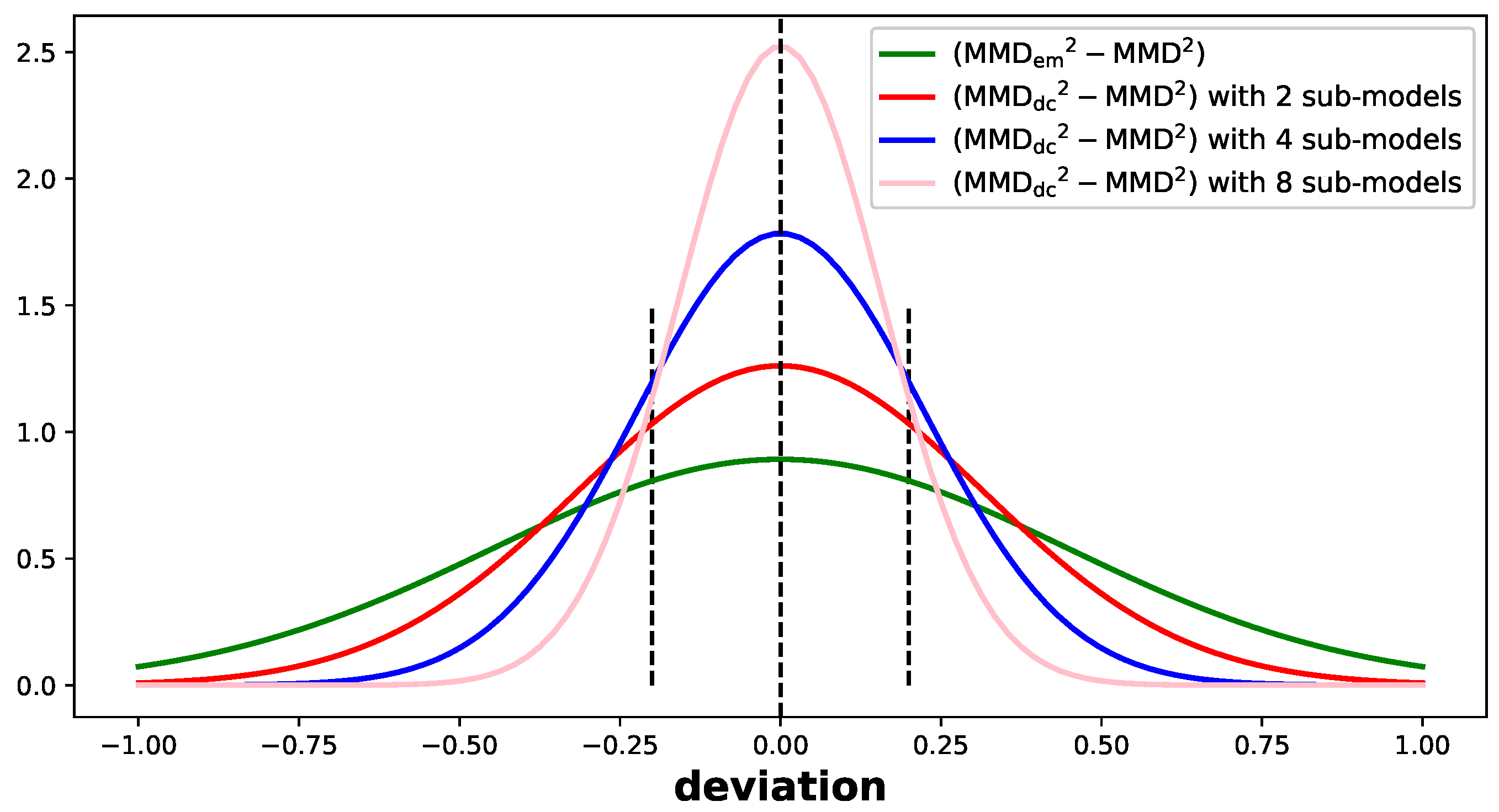
  • Based on the deviation between empirical estimate and expected value in [16], we analyze and find that the large deviation exists in original MMD-GANs, which shows that sample size used in each training iteration is not sufficient to make precise evaluation.
  • We propose DC-IPM-GANs, a novel method to constrain the loss function to tight bound on the deviation between empirical estimate and expected value of MMD. Compared to the original MMD-GANs, the loss function of DC-MMD-GANs with tighter deviation bound can measure the distance between generated distribution and target distribution more precisely, and provide more precise gradients for updating networks, which accelerates the training process. The multiple sub-models DC-MMD-GANs occupy multiple distributed computing resources. Compared to expanding the batch size on original MMD-GANs directly, the training score of DC-MMD-GANs is close to the score of MMD-GANs using less time.
  • Experimental results show that DC-MMD-GANs can be trained efficiently compared to the original MMD-GANs.
The rest of the paper is outlined as follows. Related work is shown in Section 2. The proposed method is given in Section 3. In Section 4, we present the results of experiments. Section 5 is the conclusion of the paper.

2. Related Work

2.1. MMD

As a class of IPM [9], MMD measures the distance between mean embedding of probability measures in RKHS, which is induced by a characteristic kernel [21,22]. MMD is defined as
MMD P r , Q s = sup f F , f H k 1 E r P r f ( r ) E s Q s f ( s ) ,
where H k is RKHS and F is a “unit ball” in H k . The “unit ball” means that the value of f ( · ) in RKHS is less than or equal to 1. H k is uniquely associated with a characteristic continuous kernel function k ( · , · ) , such as Gaussian radial-basis-function kernel
k σ r b f ( r , s ) = exp 1 2 σ 2 r s 2
where σ is the bandwidth.

2.2. GANs

The framework of GANs is a combination of implicit generative model and two-sample test. Generator generates fake data. Discriminator attempts to decide whether the fake-data distribution and real-data distribution are different, which is consistent with the goal of two-sample test. The choice of distance applied in GANs is closely related to the generating power, based on which we divide current variants of GANs into two sorts. The first class of GANs adopts statistical divergences as loss functions. The pioneering GANs use Jensen-Shannon divergence [1]. The distance used in least-squares GANs [23] turns out to be a variant of Pearson χ 2 divergence. Furthermore, [6] showed that all f-divergences can act as distances of GANs. IPM is the second class of loss function used in GANs, which has already been stated in Section 1. Some canonical models are WGANs [4,10], Fisher GAN [24], Sobolev GAN [11], McGAN [13], and so on.

2.3. MMD-GANs

Generative models using MMD as loss function contain many kinds of combinations [25,26,27,28]. MMD-GANs evaluate MMD for features extracted from discriminator and obtain competitive performance [14,15]. MMD in Equation (2) is defined as a form of expectation which needs to be replaced by unbiased empirical estimate using kernel function when used in MMD-GANs. The direct result of unbiased empirical estimate using kernel function is squared form: MMD em 2 . Using MMD em 2 and MMD em are equivalent for training MMD-GANs. Given target distribution P r , MMD-GANs generate fake distribution Q s to mimic P r . In MMD-GANs [14], the actual loss function is
min G min D MMD em 2 R , G ( Z ) ) ,
where R = { r i } i = 1 n , r P r i.i.d., and Z Uniform ( [ 1 , 1 ] 128 ) . G is generator and D is discriminator. Let G ( Z ) = S and S = { s i } i = 1 m , s Q s i.i.d.. According to [14], MMD em 2 is calculated as
MMD em 2 ( R , S ) = 1 m ( m 1 ) i = 1 m j i m k D ( s i , s j ) + 1 m ( m 1 ) i = 1 m j i m k D ( r i , r j ) 2 m 2 i = 1 m j = 1 m k D ( s i , r j ) ,
where k D ( · , · ) = k ( D ( · ) , D ( · ) ) . k ( · , · ) is kernel function, and m is batch size.
However, training troubles from GANs also surround MMD-GANs unavoidably. The work of [29] devised a suitable method that restricts precise and analytical regularizer on gradients to stabilize and accelerate training without additional cost. For the same purpose, [30] defined a bounded Gaussian kernel and repulsive loss function to stabilize the training of MMD-GANs.

3. Divide and Conquer MMD-GANs

In this section, we present the DC-MMD-GANs. First of all, we provide a detailed analysis of bound on the deviation between empirical estimate and expected value of MMD which shows that improving the accuracy of loss function value is extremely necessary in MMD-GANs. Secondly, we propose a novel divide-and-conquer method, which can expand the sample size of MMD-GANs indirectly and provide a more precise loss function value, to accelerate the training.
There is a deviation between MMD em 2 and MMD 2 according to [16]
Pr { MMD em 2 R , S MMD 2 P r , Q s > t } exp t 2 m 16 K 2 ,
where K is the maximum value of kernel function k ( · , · ) , Pr is the probability that deviation exceeds t, and t is deviation threshold. According to Equation (6), the deviation between MMD em 2 and MMD 2 is closely related to batch size m: MMD em 2 is approaching gradually to expectation as sample size increases.
Generally, the sample size in the region of the two-sample test is large enough because the two-sample test usually uses simple distribution with low-dimensional data, which could guarantee the quality of the two-sample test. In contrast, the sample size in the deep network model is generally not large due to complex training data. According to [31], the deviation between MMD em 2 and MMD 2 converges in a Gaussian distribution as
MMD em 2 MMD 2 D N ( 0 , σ u 2 m 1 ) ,
where D means converging to a distribution, and m is batch size. σ u 2 is the variance whose value is only related to Q s and P r . Supposing that the two distributions are completely different, and the data is same in a distribution, the minimum value of the kernel function k ( s i , r j ) in Equation (5) is 0, which means that the two distributions have no relation, i.e., the minimum value of cross term between two distributions in expression of Equation (5) is 0. The maximum value of kernel function is 1, which means that the two distributions are same. Therefore, the values of k ( s i , s j ) and k ( r i , r j ) equal to 1. In this case, the maximum of MMD em 2 is
max MMD em 2 ( R , S ) = 2 m m 1 .
When m , the maximum of MMD em 2 equals to 2.
Figure 1 shows that bound on the deviation between empirical estimate and expected value of MMD becomes tighter as the sample size increase. The deviation in Figure 1 (e.g., 0.1, 0.2, ..., 0.5) is non-negligible for the MMD em 2 whose maximum is only 2. Generally, the value of MMD em 2 in MMD-GANs is less than 2 and gets smaller as the number of iterations increases, while the deviation does not vanish. So, the impact of deviation will intensify during training. We select a point of the curve from Figure 1 for example: ( 64 , 0.4868 ) . The meaning of this point is: when batch size in MMD-GANs is set to 64, there will be 48.68 % probability that deviation between MMD 2 and MMD em 2 exceeds 0.3 , which is unacceptable for training. Generally, batch size in MMD-GANs does not exceed 128 (e.g., 32, 64, 128) [14,29], which cannot be expanded directly and lead to large deviation. Batch size cannot be expanded directly with complex training data and limited computational budget. We find that the B-test [31] can obtain a more precise empirical estimate of MMD by computing an average over empirical estimates calculated on subsets. Inspired by the divide-and-conquer strategy for kernel methods [17,18,19,20], we propose a divide-and-conquer generative model, DC-MMD-GANs. We partition training images into c subsets { R 1 , R 2 , . . . , R c } using auto-encoder and k-means in the latent space. The sub-models conduct forward propagation using different subsets independently. The loss function values of sub-models are integrated and used to calculate a new weight-sum loss to update the all sub-models synchronously. The framework of our proposed method is shown in Figure 2.
The purpose of dividing training data is to reduce the loss of information and improve the generating performance. The advantages of division task is shown as follows:
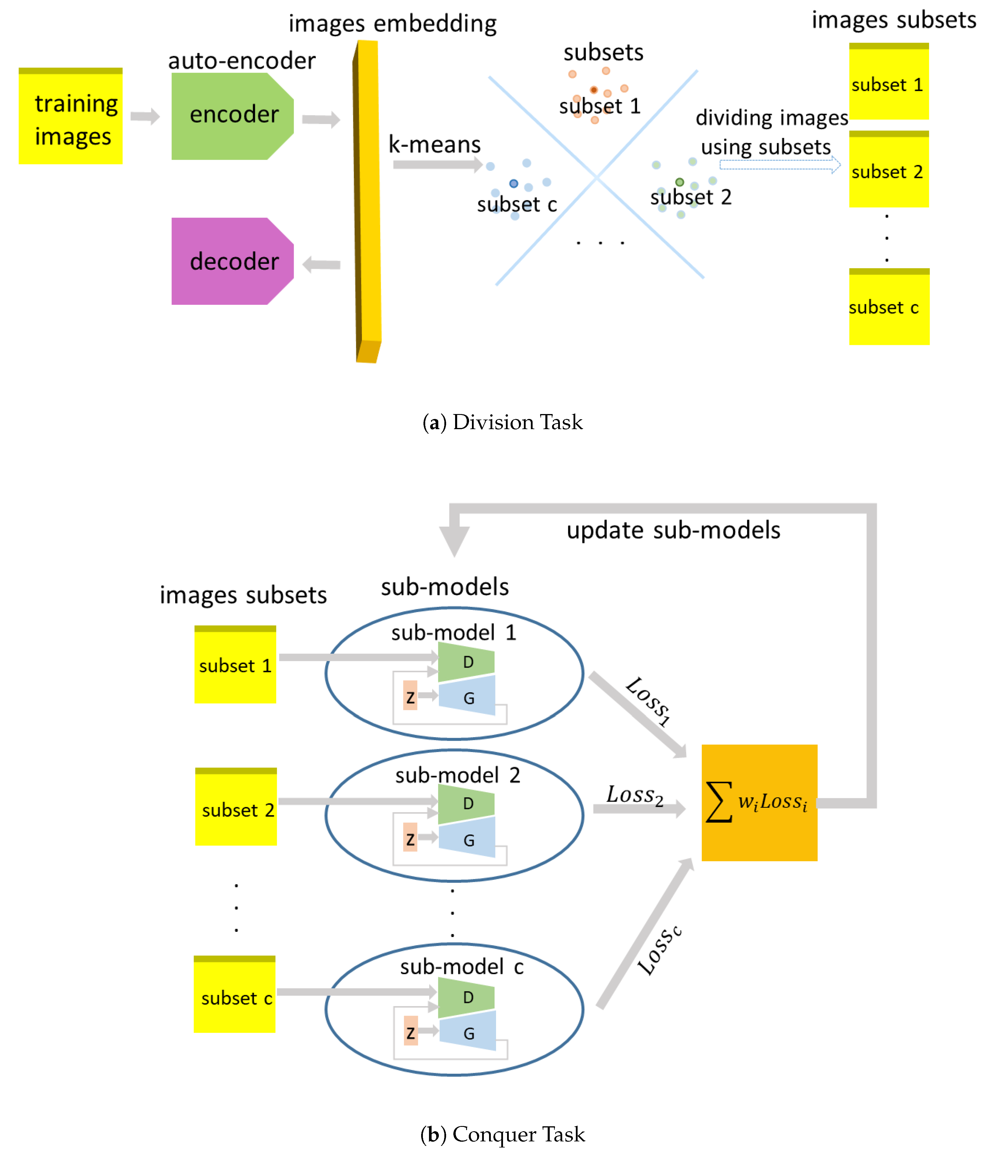
  • Each subset of training images divided by k-means owns minimum distance in embedding space. The correlation between each subset is reduced. MMD em 2 ( R i , R j ) i j between each subset gets bigger. R i and R j are different batches of training images of different subset. According to Equation (5), the third term in MMD em 2 ( R i , R j ) i j will be reduced, which is the cross term between different subsets and cannot be obtained due to independent sub-model. From this perspective, auto-encoder and k-means help to reduce the loss of information of training images during training process.
  • Each subset of training images is used to train on one sub-model. All training images are learned more quickly compared with the baseline model.
  • According to different cluster of embeddings, we divide images into subsets, which can be viewed as different categories. Divided subsets contain different information of clustered embeddings, which is shown to improve training of GANs [32]. A pre-trained model such as the combination of auto-encoder and k-means is shown to be benefit for generator to produce high-quality images [33].
The target distribution P r is primarily supported by low-dimensional manifolds [10]. We try to learn useful feature representation, which can represent the essence of the target distribution. Auto-encoder has enough capacity to capture prominent information of target data. By mapping training images space R d into low-dimensional embedding space R e , the encoder outputs the most representative embedding e [34]. Furthermore, auto-encoder disentangles complex variations of training images which is beneficial for division tasks [35].
We train auto-encoder with all training images by minimizing mean squared errors (MSE) between training data and reconstructed samples. The dimension of the output layer of the encoder was set to 256 with three convolution layers and two fully connected layers. Auto-encoder is composed of encoder and decoder, which is shown as follows
min D c , E c L o s s = 1 m i = 1 m r i D c E c r i 2 , e = E c R , e R e , R ^ r e = D c E c R ,
where E c ( · ) is encoder and D c ( · ) is decoder. R ^ r e is reconstructed data. m is batch size and R = { r i } i = 1 n , r P r i.i.d. We freeze auto-encoder parameters and pass all training images to well-trained auto-encoder. Each image r i is mapped to a vector of embedding e i . E a l l is a set containing all embedding e i .
Based on learned embedding representation, we conduct k-means on E a l l and obtain c clusters: E i , i { 1 , . . . , c } . Hereby training images are divided into c subsets R i , i { 1 , . . . , c } respectively according to clustered set of embedding. Each subset will be fed to a sub-model. Each sub-model is trained independently.
For conquer task, we adopt a weighted-sum unbiased empirical estimate of MMD 2 with tighter deviation bound: MMD dc 2 , which can provide more precise gradients for training. All sub-problems of training independently, we integrate the empirical estimation { MMD em 2 ( R 1 , S 1 ) , MMD em 2 ( R 2 , S 2 ) , . . . , MMD em 2 ( R c , S c ) } . R c is a batch of training images and S c is a batch of generated images generated by the c-th sub-model. We compute a weight-sum value of all estimate: MMD dc 2 , with a tighter deviation bound. We set the weight parameter to 1 c .
MMD dc 2 ( R , S ) = i = 1 c w i MMD em 2 ( R i , S i ) .
Each sub-model is updated synchronously by optimizing MMD dc 2
min G s u b min D s u b MMD dc 2 R , S ,
where G s u b is generator and D s u b is discriminator of sub-model. As shown in the Theorem 1, the new loss function MMD dc 2 can be seen as an unbiased estimator of expected value MMD 2 . Therefore, optimizing MMD dc 2 can give correct direction of convergence when training DC-MMD-GANs.
Theorem1. 
Assuming that i = 1 c w i = 1 , MMD dc 2 is an unbiased estimator of MMD 2 .
Proof of Theorem 1. 
According to [16], for each MMD em 2 ( R i , S i ) , E ( MMD em 2 ( R i , S i ) ) = MMD 2 .
E ( MMD dc 2 ( R , S ) ) = i = 1 c w i E ( MMD em 2 ( R i , S i ) = i = 1 c w i MMD 2 = MMD 2 .
The calculation of MMD dc 2 can be seen as a type of unbiased estimator used in the B-test [31], which is an average over empirical estimate of MMD 2 computed on subsets. According to Equation (5), MMD em 2 with batch size equaling to m can be obtained by computing m 2 terms of k ( · , · ) . MMD em 2 with batch size equaling to c m can be obtained by computing c 2 m 2 terms. By using the divide-and-conquer strategy, MMD dc 2 is computed using c MMD em 2 according to Equation (10). So MMD dc 2 can be obtained by computing c m 2 terms. Compared to compute the MMD em 2 with batch size equaling to c m , we avoid the calculation of cross terms when we calculated MMD dc 2 . The cross terms are the information between different subsets and has been reduced by the division task. MMD dc 2 has same deviation bound as MMD em 2 with batch size equaling to c m according to [31]. Therefore, DC-MMD-GANs using MMD dc 2 can be viewed expanding batch size from m to c m effectively with less computation amount compared to MMD em 2 with batch size equaling to c m and obtain a tighter deviation bound as is shown in Equation (12) compared to MMD em 2 with batch size equaling to m. Under the same Pr , MMD dc 2 is more accurate than MMD em 2 because the deviation t between MMD dc 2 and MMD 2 is smaller than deviation between MMD em 2 and MMD 2 .
Pr { MMD dc 2 R , S MMD 2 P r , Q s > t } exp t 2 c m 16 K 2 .
According to [31], deviation between MMD dc 2 and MMD 2 converges in a Gaussian distribution with lower variance [31] compared to original model. As shown in Figure 3, MMD dc 2 has a tighter deviation bound compared to the deviation between MMD em 2 and MMD 2 . As the number of sub-models increases, the deviation bound becomes tighter, which is shown as
MMD dc 2 MMD 2 D N ( 0 , σ u 2 ( c m ) 1 ) .
where σ u 2 is the variance whose value is only related to Q s and P r . P r is same between models. Q s is approximately the same because it is approaching P r . Therefore, σ u 2 is same as the variance in Equation (7).

4. Experiment

In this section, we conducted experiments on unsupervised image generation to evaluate the performance of proposed DC-MMD-GANs. The experiments are conducted on two popular datasets, CIFAR-10 [36] (10 categories, 32 × 32 ), and CelebA [37] (face images, resized and cropped to 160 × 160 ). Models were trained on Nvidia GTX 1080Ti GPUs. CelebA was trained on a generator with 10-layer ResNet as in [29] and a discriminator with 5-layer DCGAN architecture [2]. For CIFAR-10, we used a standard CNN structure of [38], which contains a 4-layer generator and a 7-layer discriminator.
To compare generation quality of GANs, we adopted Fréchet Inception Distance (FID) [39] and Kernel Inception Distance (KID) [14] as evaluation metrics. FID measures similarity between generated images and real images. FID fits intermediate representations of generated images and real images into two multidimensional Gaussian distributions and computes Wasserstein-2 distance between the two distributions. KID adopts a squared polynomial-kernel MMD between generated images and real images as evaluation distance. The lower scores of FID and KID, the better generation quality will be. The number of real images used in computing FID and KID was set to 10,000. According to [39], the FID d FID ( , ) is shown as
d FID ( ( m r , C r ) , ( m s , C s ) ) = m r m s 2 2 + T r ( C r + C s 2 ( C r C s ) 1 2 ) 1 2
where ( m r , C r ) is Gaussian distribution obtained from P r and ( m s , C s ) is obtained from Q s . According to [29], the KID d KID ( , ) is shown as
d KID ( R , S ) = MMD em 2 ( ψ ( R ) , ψ ( S ) )
where ψ ( · ) is representation of generated images and real images in the Inception model [40].
For CelebA, auto-encoder was pre-trained for 20,000 iterations on 20,000 training images. We got embedding of all images by auto-encoder. According to the clusters of k-means on the learned embedding by auto-encoder, we divided 10,000 images into 2, 4 and 8 subsets. For CIFAR-10, auto-encoder was pre-trained for 10,000 iterations on 60,000 images and divided 30,000 images into 2, 4 and 8 subsets. As a comparison to DC-MMD-GANs, we also trained the standard model which is equivalent to the proposed model when c = 1 .
DC-MMD-GANs contain DC-SMMD-GAN and DC-MMD-GAN. We used 2, 4, and 8 sub-models in DC-MMD-GAN and DC-SMMD-GAN. We compared two related GANs models, MMD-GAN [14,15] and Scaled MMD-GAN (SMMD-GAN) [29].
We limited the number of training iterations to 15,000 for CelebA to compare learning efficiency and evaluation scores between different models. Because the generating quality of DC-MMD-GANs is high when the training step is 15,000. For CIFAR-10, we limited number of training iterations to 5000 in DC-SMMD-GAN and DC-MMD-GAN. To show differences in the performance of each model clearly, we computed FID and KID every 500 generator iterations. The learning rate was set to 0.0001. The batch size of each sub-model was set to 64. According to [14], the discriminator updated 5 times during 1 generator iteration. According to [29], the dimension of discriminator outputs was set to 1 in DC-SMMD-GAN, while it was 16 in DC-MMD-GAN. DC-SMMD-GAN used a radial-basis-function kernel with bandwidth equaling to 0.5. DC-MMD-GAN used a mixture of rational quadratic kernels as in [14]. In DC-MMD-GAN, the gradient penalty and L 2 penalty on discriminator layers were both set to 1. The Adam optimizer was used for all models with β 1 = 0.5 , β 2 = 0.9 .
Figure 4 shows FID and KID of CelebA trained on these models. According to score curves in Figure 4, we find that curves of DC-MMD-GANs drop faster when compared to the original models. The training process of DC-MMD-GANs is faster than the original model. For example, in Figure 4a, the FID score of DC-SMMD-GAN with 8 models reaches 40 in about 6500 iterations on celebA. The FID score of original model reaches 40 in about 11,500 iterations, which is 5000 iterations more than the DC-SMMD-GANs with 8 sub-models. The FID score can reach 40 in fewer iterations as the sub-model increases (about 8500 iterations of DC-SMMD-GAN with 4 sub-models and 9500 iterations of DC-SMMD-GAN with 2 sub-models). We can get the consistent observation on other figures. Under the same number of iterations, we find that in most cases, the score of DC-MMD-GANs is better than the original models. The DC-MMD-GANs with 4 sub-models perform better than the 2-sub-models ones. The training results of DC-MMD-GANs with more sub-models are relatively better because of the more precise value of loss function. However, compared to the promotion of performance from original models to 4-sub-model DC-MMD-GANs, the improvement from 4-sub-models DC-MMD-GANs to 8-sub-models ones is not obvious. Partly because the improvement of the tightness from 4-sub-models DC-MMD-GANs to 8-sub-models ones is not obvious, which can be also observed in Figure 1. Figure 5 and Figure 6 shows the generated images of CelebA after 15,000 iterations. We find that under the same number of iterations, DC-MMD-GANs can generate higher quality images while parts of the images from original models are blurred. Under the limited iterations, DC-MMD-GANs can learn more detail from training images and generate more realistic images. However, the resolution of CIFAR-10 is low. It is hard to find how the DC-MMD-GANs improve the generating quality so we did not show the generated images of CIFAR-10. However, the improvement of DC-MMD-GANs can be observed in Figure 7. Figure 7 presents FID and KID of CIFAR-10 trained on these models. DC-MMD-GANs can converge faster on CIFAR-10, which is consistent with the results of training on CelebA.
For CelebA, the GANs training time is 14.70 h in DC-SMMD-GANs and SMMD-GANs. In DC-MMD-GANs and MMD-GANs, the training time is 18.10 h. The time for auto-encoder training and conducting k-means (division task) is 1.57 h. Compared to training time of GANs, the division task can be omitted. For CIFAR-10, the training time is 0.7 h in DC-SMMD-GANs and 0.90 h in DC-MMD-GANs. The time of division task is 0.10 h, which can be omitted. The time used for auto-encoder training and k-means can be omitted because: (1) Compared to the GANs training time, division task takes a short period of time which will be shown in experiment. (2) The auto-encoder is trained once in each dataset and time of conducting k-means can be omitted.
We compared the training score of 2-sub-models DC-MMD-GANs with batch size equaling to 32, 4-sub-models DC-MMD-GANs with batch size equaling to 16, 8-sub-models DC-MMD-GANs with batch size equaling to 8, and MMD-GANs with batch size equaling to 64. Figure 8 and Figure 9 shows FID and KID of CelebA and CIFAR-10 trained on these models. According to the score curves, we find that the training score of DC-MMD-GANs is close to the MMD-GANs. Table 1 shows the training time of DC-MMD-GANs can be reduced as the number of sub-models increases compared to MMD-GANs. The training time of DC-MMD-GANs is reduced because: (1) the strategy of DC-MMD-GANs is parallel divide-and-conquer (2) MMD dc 2 can be obtained with less computation amount compared to MMD em 2 with batch size equaling to cm which can accelerate the training process.

5. Conclusions

In this paper, we connected the improvement of accuracy of statistic value with efficient training of GANs, and proposed a brand-new divide-and-conquer GANs model, DC-MMD-GANs, which is a tradeoff between training time and computing resources. Based on the insight of large deviation existing in MMD-GANs, we showed the loss function of the DC-MMD-GANs owns a tighter deviation bound, which may open the door for research into optimization of generative models from statistical perspectives. Experimental results have shown that the DC-MMD-GANs can be trained efficiently compared to the standard MMD-GANs. However, the model of DC-MMD-GANs still has some limitations, such as the division task, which takes up some pre-training time and resources. One interesting direction of future study is reducing the occupation of division task and choosing the best number of sub-models.

Author Contributions

Conceptualization, Y.Z.; methodology, Z.Z.; software, X.L.; validation, Q.L.; formal analysis, S.H.; writing, Z.Z. All authors have read and agreed to the published version of the manuscript.

Funding

This work was supported in part by the National Natural Science Foundation of China under Grant 61501069, and in part by the special project of technological innovation and application development of Chongqing (NO.cstc2019jscx-msxmX0167).

Conflicts of Interest

The authors declare no conflict of interest.

References

  1. Goodfellow, I.; Pouget-Abadie, J.; Mirza, M.; Xu, B.; Warde-Farley, D.; Ozair, S.; Courville, A.; Bengio, Y. Generative Adversarial Nets. In Proceedings of the Conference on Advances in Neural Information Processing Systems, Generative Adversarial Nets, Montréal, QC, Canada, 8–13 December 2014; pp. 2672–2680. [Google Scholar]
  2. Radford, A.; Metz, L.; Chintala, S. Unsupervised representation learning with deep convolutional generative adversarial networks. arXiv 2015, arXiv:1511.06434. [Google Scholar]
  3. Arjovsky, M.; Bottou, L. Towards Principled Methods for Training Generative Adversarial Networks. arXiv 2017, arXiv:1701.04862. [Google Scholar]
  4. Gulrajani, I.; Ahmed, F.; Arjovsky, M.; Dumoulin, V.; Courville, A.C. Improved training of Wasserstein GANs. In Proceedings of the Conference on Advances in Neural Information Processing Systems, Long Beach, CA, USA, 4–9 December 2017; pp. 5767–5777. [Google Scholar]
  5. Karras, T.; Aila, T.; Laine, S.; Lehtinen, J. Progressive growing of GANs for improved quality, stability, and variation. arXiv 2017, arXiv:1710.10196. [Google Scholar]
  6. Nowozin, S.; Cseke, B.; Tomioka, R. f-GAN: Training generative neural samplers using variational divergence minimization. In Proceedings of the Conference on Advances in Neural Information Processing Systems, Barcelona, Spain, 5–10 December 2016; pp. 271–279. [Google Scholar]
  7. Ledig, C.; Theis, L.; Huszár, F.; Caballero, J.; Cunningham, A.; Acosta, A.; Aitken, A.; Tejani, A.; Totz, J.; Wang, Z. Photo-realistic single image super-resolution using a generative adversarial network. In Proceedings of the IEEE Conference on Computer Vision and Pattern Recognition, Maui, HI, USA, 21–26 July 2017; pp. 4681–4690. [Google Scholar]
  8. Wang, S.; Zhang, L.; Fu, J. Adversarial transfer learning for cross-domain visual recognition. Knowl. Based Syst. 2020, 204, 106258. [Google Scholar] [CrossRef]
  9. Müller, A. Integral probability metrics and their generating classes of functions. Adv. Appl. Probab. 1997, 29, 429–443. [Google Scholar] [CrossRef]
  10. Arjovsky, M.; Chintala, S.; Bottou, L. Wasserstein generative adversarial networks. In Proceedings of the International Conference on Machine Learning, Sydney, Australia, 6–11 August 2017; pp. 214–223. [Google Scholar]
  11. Mroueh, Y.; Li, C.L.; Sercu, T.; Raj, A.; Cheng, Y. Sobolev GAN. In Proceedings of the International Conference on Learning Representations, Vancouver, BC, Canada, 30 April–3 May 2018. [Google Scholar]
  12. Genevay, A.; Peyre, G.; Cuturi, M. Learning Generative Models with Sinkhorn Divergences. In Proceedings of the International Conference on Artificial Intelligence and Statistics, Canary Islands, Spain, 9–11 April 2018; pp. 1608–1617. [Google Scholar]
  13. Mroueh, Y.; Sercu, T.; Goel, V. McGAN: Mean and Covariance Feature Matching GAN. In Proceedings of the International Conference on Machine Learning, Sydney, Australia, 6–11 August 2017; pp. 2527–2535. [Google Scholar]
  14. Bińkowski, M.; Sutherland, D.; Arbel, M.; Gretton, A. Demystifying MMD GANs. In Proceedings of the International Conference on Learning Representations, Vancouver, BC, Canada, 30 April–3 May 2018. [Google Scholar]
  15. Li, C.L.; Chang, W.C.; Cheng, Y.; Yang, Y.; Póczos, B. MMD GAN: Towards deeper understanding of moment matching network. In Proceedings of the Conference on Advances in Neural Information Processing Systems, Long Beach, CA, USA, 4–9 December 2017; pp. 2203–2213. [Google Scholar]
  16. Gretton, A.; Borgwardt, K.M.; Rasch, M.J.; Schölkopf, B.; Smola, A. A kernel two-sample test. J. Mach. Learn. Res. 2012, 13, 723–773. [Google Scholar]
  17. Hsieh, C.J.; Si, S.; Dhillon, I. A divide-and-conquer solver for kernel support vector machines. In Proceedings of the International Conference on Machine Learning, Beijing, China, 21–26 June 2014; pp. 566–574. [Google Scholar]
  18. Hsieh, C.J.; Si, S.; Dhillon, I.S. Fast prediction for large-scale kernel machines. In Proceedings of the Conference on Advances in Neural Information Processing Systems, Montréal, BC, Canada, 8–13 December 2014; pp. 3689–3697. [Google Scholar]
  19. Tandon, R.; Si, S.; Ravikumar, P.; Dhillon, I. Kernel ridge regression via partitioning. arXiv 2016, arXiv:1608.01976. [Google Scholar]
  20. Si, S.; Hsieh, C.J.; Dhillon, I.S. Memory efficient kernel approximation. J. Mach. Learn. Res 2017, 18, 682–713. [Google Scholar]
  21. Fukumizu, K.; Gretton, A.; Lanckriet, G.R.; Schölkopf, B.; Sriperumbudur, B.K. Kernel choice and classifiability for RKHS embeddings of probability distributions. In Proceedings of the International Conference on Learning Representations, Vancouver, BC, Canada, 14–18 June 2009; pp. 1750–1758. [Google Scholar]
  22. Sriperumbudur, B.K.; Gretton, A.; Fukumizu, K.; Schölkopf, B.; Lanckriet, G.R. Hilbert space embeddings and metrics on probability measures. J. Mach. Learn. Res. 2010, 11, 1517–1561. [Google Scholar]
  23. Mao, X.; Li, Q.; Xie, H.; Lau, R.Y.; Wang, Z.; Paul Smolley, S. Least squares generative adversarial networks. In Proceedings of the IEEE International Conference on Computer Vision, Venice, Italy, 22–29 October 2017; pp. 2794–2802. [Google Scholar]
  24. Mroueh, Y.; Sercu, T. Fisher GAN. In Proceedings of the International Conference on Advances in Neural Information Processing Systems, Long Beach, CA, USA, 4–9 December 2017; pp. 2513–2523. [Google Scholar]
  25. Li, Y.; Swersky, K.; Zemel, R. Generative moment matching networks. In Proceedings of the International Conference on Machine Learning, Lille, France, 6–11 July 2015; pp. 1718–1727. [Google Scholar]
  26. Sutherland, D.J.; Tung, H.Y.; Strathmann, H.; De, S.; Ramdas, A.; Smola, A.; Gretton, A. Generative models and model criticism via optimized maximum mean discrepancy. arXiv 2016, arXiv:1611.04488. [Google Scholar]
  27. Salimans, T.; Goodfellow, I.; Zaremba, W.; Cheung, V.; Radford, A.; Chen, X.; Chen, X. Improved Techniques for Training GANs. In Proceedings of the International Conference on Advances in Neural Information Processing Systems, Barcelona, Spain, 5–10 December 2016; pp. 2234–2242. [Google Scholar]
  28. Dziugaite, G.K.; Roy, D.M.; Ghahramani, Z. Training generative neural networks via maximum mean discrepancy optimization. arXiv 2016, arXiv:1505.03906. [Google Scholar]
  29. Arbel, M.; Sutherland, D.; Bińkowski, M.; Gretton, A. On gradient regularizers for MMD GANs. In Proceedings of the International Conference on Advances in Neural Information Processing Systems, Montréal, BC, Canada, 3–8 December 2018; pp. 6700–6710. [Google Scholar]
  30. Wang, W.; Sun, Y.; Halgamuge, S. Improving MMD-GAN Training with Repulsive Loss Function. In Proceedings of the International Conference on Learning Representations, New Orleans, LA, USA, 6–9 May 2019. [Google Scholar]
  31. Zaremba, W.; Gretton, A.; Blaschko, M. B-test: A Non-parametric, Low Variance Kernel Two-sample Test. In Proceedings of the International Conference on Advances in Neural Information Processing Systems, Lake Tahoe, NV, USA, 5–8 December 2013; pp. 755–763. [Google Scholar]
  32. Grinblat, G.L.; Uzal, L.C.; Granitto, P.M. Class-splitting generative adversarial networks. arXiv 2017, arXiv:1709.07359. [Google Scholar]
  33. Zhang, H.; Xu, T.; Li, H.; Zhang, S.; Wang, X.; Huang, X.; Metaxas, D.N. StackGAN: Text to photo-realistic image synthesis with stacked generative adversarial networks. In Proceedings of the IEEE International Conference on Computer Vision, Venice, Italy, 22–29 October 2017; pp. 5907–5915. [Google Scholar]
  34. Kingma, D.P.; Welling, M. Auto-encoding variational bayes. arXiv 2013, arXiv:1312.6114. [Google Scholar]
  35. Bengio, Y.; Mesnil, G.; Dauphin, Y.; Rifai, S. Better mixing via deep representations. In Proceedings of the International Conference on Machine Learning, Atlanta, GA, USA, 17–19 June 2013; pp. 552–560. [Google Scholar]
  36. Krizhevsky, A.; Hinton, G. Learning Multiple Layers of Features from Tiny Images. Master’s Thesis, University of Toronto, Toronto, ON, Canada, 2009. [Google Scholar]
  37. Liu, Z.; Luo, P.; Wang, X.; Tang, X. Deep learning face attributes in the wild. In Proceedings of the IEEE International Conference on Computer Vision, Santiago, Chile, 11–18 December 2015; pp. 3730–3738. [Google Scholar]
  38. Miyato, T.; Kataoka, T.; Koyama, M.; Yoshida, Y. Spectral normalization for generative adversarial networks. arXiv 2018, arXiv:1802.05957. [Google Scholar]
  39. Heusel, M.; Ramsauer, H.; Unterthiner, T.; Nessler, B.; Hochreiter, S. GANs trained by a two time-scale update rule converge to a local nash equilibrium. In Proceedings of the International Conference on Advances in Neural Information Processing Systems, Long Beach, CA, USA, 4–9 December 2017; pp. 6626–6637. [Google Scholar]
  40. Szegedy, C.; Vanhoucke, V.; Ioffe, S.; Shlens, J.; Wojna, Z. Rethinking the Inception Architecture for Computer Vision. In Proceedings of the International Conference on Computer Vision and Pattern Recognition (CVPR), Las Vegas, NV, USA, 26 June–1 July 2016; pp. 2818–2826. [Google Scholar]
Figure 1. Illustration of the probability of | MMD em 2 MMD 2 | exceeding deviation t. The horizontal axis is batch size. The number next to the curve is the probability of exceeding different deviation t under the specific batch size. The figure shows that the probability of exceeding large deviation is high under the small batch size. Generally, the batch size in MMD-GANs is less than 128 and the deviation of loss function is large. Under the same deviation t, the probability of exceeding t decreases with increasing of batch size.
Applsci 10 06405 g001
Figure 2. The structure of the DC-MMD-GANs. We train an auto-encoder and get embedding of training images from the output of encoder. K-means clusters on the embedding of auto-encoder into adaptive subsets. We divide the training images into subsets according to embedding subsets. Each sub-model is trained independently with different subsets. The master node computes the new weight-sum loss function and obtains precise empirical estimate based on output of sub-models.
Applsci 10 06405 g002
Figure 3. The distribution of deviation between the square of empirical estimate and MMD 2 . Besides the original model, we set the number of sub-models of DC-MMD-GANs to 2, 4, and 8. The distribution of deviation of original MMD-GANs (green curve) have high variance, which means that the loss function of MMD-GANs has loose deviation bound. The loss function of DC-MMD-GANs has relatively tight deviation bound and the bound becomes tighter as the number of sub-models increases.
Applsci 10 06405 g003
Figure 4. The evolution of FID and KID as the number of iterations increases when trained on celebA. Both on DC-SMMD-GAN and DC-MMD-GAN, the proposed methods can converge faster and obtain better evaluation score. Under the same number of iterations, the evaluation score becomes better as the number of sub-models increases. The improvement is obvious from the original models to the 4-sub-model methods. However, there is not obvious improvement when we add the number of sub-models to 8.
Applsci 10 06405 g004
Figure 5. Images generated by different models trained on CelebA when the number of iterations is 15,000. DC-SMMD-GANs generate more realistic images while parts of images from the original models are blurred.
Applsci 10 06405 g005
Figure 6. DC-MMD-GAN generate more realistic images while parts of images from the original models are blurred.
Applsci 10 06405 g006
Figure 7. The evolution of FID and KID as the number of iterations increases when trained on CIFAR-10. Compared to the original models, the proposed methods can make the training more efficiently.
Applsci 10 06405 g007
Figure 8. The evolution of FID and KID as the number of iterations increases when trained on celebA. Compared to the score of MMD-GANs with batch size equaling to cm, DC-MMD-GANs reach competitive score with less training time.
Applsci 10 06405 g008
Figure 9. The evolution of FID and KID as the number of iterations increases when trained on CIFAR-10. Compared to the score of MMD-GANs with batch size equaling to cm, DC-MMD-GANs reach competitive score with less training time. DC-MMD-GANs accelerate the training process.
Applsci 10 06405 g009
Table 1. Training time of different models on CelebA and CIFAR-10.
ModelCelebACIFAR-10
SMMD-GAN with batch size = 6414.70 h0.73 h
2-sub-models DC-SMMD-GAN with batch size = 327.80 h0.53 h
4-sub-models DC-SMMD-GAN with batch size = 165.10 h0.41 h
8-sub-models DC-SMMD-GAN with batch size = 83.60 h0.34 h
MMD-GAN with batch size = 6418.10 h0.90 h
2-sub-models DC-MMD-GAN with batch size = 329.75 h0.61 h
4-sub-models DC-MMD-GAN with batch size = 166.10 h0.47 h
8-sub-models DC-MMD-GAN with batch size = 84.50 h0.40 h

