An Approach on Velocity and Stability Control of a Two-Wheeled Robotic Wheelchair

Abstract

Conventional robotic wheelchairs (three or four-wheeled) which are statically stable are poor in mobility. Though a two-wheeled robotic wheelchair has better mobility, it is not statically stable and needs an active stability controller. In addition to mobility and stability, velocity control is also important for the operation of a wheelchair. Conventional stability and velocity controllers rely on the motion of the wheels and require high driving torque and power. In this paper, this problem is tackled by adding a compact pendulum-like movable mechanism whose main function is for stability control. Its motion and those of the wheels are controlled through a quasi-sliding mode control approach to achieve a simultaneous velocity and stability control with much less driving torque and power. Simulation results are presented to show the effectiveness of the proposed controller.

1. Introduction

Compared to conventional manually operated wheelchairs, motorized wheelchairs equipped with an automatic control system (so-called robotic wheelchairs) have many advantages. For example, they have better navigation capabilities and can respond to different motion requirements autonomously [1,2,3]. Most conventional robotic wheelchairs contain two active driving wheels and two passive casters [4]. Though casters enhance the stability of the wheelchair, they have a negative effect on its mobility [5,6,7]. To solve this problem, caster-free two-wheeled robotic wheelchair equipped with an active stability controller was proposed [8,9,10].

There are several types of two-wheeled wheelchairs with special features. The iBot has four wheels, but can be converted to a two-wheeled wheelchair by lifting up its two caster wheels [11,12,13]. The height of the rider seat increases as a result. A patented iBalance^TM technology, a synthesis of computers and gyroscope, is used to keep the wheelchair stable. A two-wheeled transportation vehicle called B2 has a self-balancing (stability) capability when it is subject to disturbances from the road. It is suitable for use on narrow roads as it can turn on the spot in a space much smaller than that needed by a conventional car [14,15].

Nonlinear controllers can be used for velocity and stability control of a two-wheeled wheelchair as its dynamic model is highly nonlinear [16]. One example is computed torque control based on nonlinear feedback and the assumption that the exact dynamic model of the system is known [17]. For the cases where the system dynamics cannot be accurately modelled, or there are external disturbances, $H_{\infty }$ which is robust against disturbances can be used [18,19]. Nonlinear $H_{\infty }$ control is developed based on the Hamilton–Jacobi–Bellman–Isaacs (HJBI) equation which is hard to solve in real-time though [20].

Another type of robust controller is sliding mode control (SMC) which has an elegant structure and is effective in disturbance rejection and is robust to system parameters variation. In this controller, the state of the closed-loop system is forced to slide along the predefined sliding surface [21,22,23]. However, it suffers chatterings in the closed-loop system states. This problem can be solved by quasi-sliding mode control (QSMC) where the non-smooth sign function used in SMC is replaced with a smooth sigmoid function to govern the switching behavior in the controller [24]. For a system whose number of inputs is less than the number of outputs (underactuated system), hierarchical sliding mode control (HSMC) can be used. In HSMC, the sliding surfaces are designed in layers which are called layer sliding surface [25].

In most controllers, the motion and stability of the wheelchair all rely on the motions of the driving wheels which need large driving torque and power [26]. Some approaches have been proposed to solve this problem. For example, the rider’s seat is made to move to enhance the wheelchair’s stability [27]. The wheelchair is designed in a way such that its center of gravity is under the driving wheels’ axis [28]. A mass under the rider’s seat moves linearly to keep the wheelchair from overturning [29]. These approaches have the drawbacks of compromising the comfort of the rider or limited effectiveness.

In this paper, an active velocity and stability controller is developed for a two-wheeled wheelchair added with a compact pendulum-like movable mechanism. The Euler–Lagrange equation is used to derive the equation of motion (EOM) of the system and a quasi-sliding mode control approach is used in the controller design. Through the proposed control scheme, the wheelchair’s velocity and stability can be controlled with driving torque and power much less than those of conventional controllers which only rely on the motions of the driving wheels. Simulation results prove the effectiveness of the proposed controller.

The rest of the paper is organized as follows. In Section 2, the structure of a two-wheeled robotic wheelchair and proposed mechanism is presented. The dynamic model of the system is introduced in Section 3. In Section 4, the controller design is proposed. In Section 5, simulation results are shown to compare the performances of the conventional and proposed methods. Conclusions are given in Section 6.

2. System Description

As shown in Figure 1, a two-wheeled wheelchair comprises a seat and two wheels. The seat is connected to the axial of the wheels through a rod. A pendulum like movable mechanism is connected to the rod through a rotating joint. There is a mass placed at the end of the pendulum. The masses of the pendulum and the rod are ignored. To describe the state of all the modules of the wheelchair, a body coordinate frame X-Y-Z is placed at the center of the wheels’ axle (O). Though Z axis is not shown in the figure, it is perpendicular to X and Y axis as determined by the right-hand rule. All moments of inertia are defined around their centre of gravity (CoG) in Z axis. The rotation angles of the wheels and the wheelchair body are measured from Y axis, while the rotation angle of the movable mechanism is measured from link OP. The nomenclature can be found in Table 1.

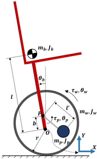
Figure 1. Two-wheeled wheelchair and proposed mechanism.

Table 1. Nomenclature.

Symbol	Description
$m_{\mathrm{w}}$	Mass of each wheel
$m_b$	Mass of body
$m_p$	Mass of movable mechanism
$J_{\mathrm{w}}$	Moment of inertia of each wheel
$J_b$	Moment of inertia of body
$J_p$	Moment of inertia of movable mechanism
O	Centre of the wheels’ axle
P	Contact point of the movable mechanism and wheelchair
r	Radius of each wheel
l	Distance from the body’s CoG to point P
$l^{\prime }$	Length of the rod of the pendulum (movable mechanism)
b	Distance from point O to point P
${\theta }_{\mathrm{w}}$	Rotation angle of the wheel
${\theta }_b$	Rotation angle of the body (pitch angle)
${\theta }_p$	Rotation angle of the pendulum
${\tau }_r$	Input torque of the right wheel
${\tau }_l$	Input torque of the left wheel
${\tau }_{\mathrm{w}}$	Total input torque of the wheels
${\tau }_p$	Input torque of the pendulum
$P_{\mathrm{w}}$	Input power of the wheels
$P_p$	Input power of the pendulum

3. Modeling of Two-Wheeled Robotic Wheelchair

3.1. Conventional Method

In a conventional method, the wheels are responsible for both the stability and velocity control of the wheelchair. The controller is based on the EOM of the system which can be derived from the Euler–Lagrange equation [30]:

$$\frac{d}{dt}(\frac{\partial T}{\partial {\dot{q}}_i})-\frac{\partial T}{\partial q_i}+\frac{\partial U}{\partial q_i}=Q_i$$

(1)

T and U are the kinetic and the potential energy of the system. $q_i$ and $Q_i$ are the generalized coordinates and the corresponding input of system respectively. Slip between the ground and wheels and friction forces in the system are neglected. Each wheel’s kinetic and potential energy can be shown as

$$T_{\mathrm{w}}=\frac{1}{2}{m}_{\mathrm{w}}{r}^2{\dot{\theta }}_{\mathrm{w}}^2+\frac{1}{2}{J}_{\mathrm{w}}{\dot{\theta }}_{\mathrm{w}}^2,U_{\mathrm{w}}=0.$$

The body’s kinetic and potential energy are

$$T_b=\frac{1}{2}{m}_b{r}^2{\dot{\theta }}_{\mathrm{w}}^2+\frac{1}{2}{m}_b{l}^2{\dot{\theta }}_b^2+m_{b}rl{\dot{\theta }}_{\mathrm{w}}{\dot{\theta }}_b\cos {\theta }_b+\frac{1}{2}{J}_b{\dot{\theta }}_b^2,U_b=m_{b}gl\cos {\theta }_b.$$

The overall kinetic and potential energy of the system is

$$T=2T_{\mathrm{w}}+T_b,U=2U_{\mathrm{w}}+U_b.$$

Through Equation (1), the EOM of the system can be derived and presented as [31]

$$\mathbf{M}(\mathbf{q})\ddot{\mathbf{q}}+\mathbf{H}(\mathbf{q},\dot{\mathbf{q}})+\mathbf{G}(\mathbf{q})=\mathbf{Q},$$

(2)

where $\mathbf{q}$ is the vector of generalized coordinates

$$\mathbf{q}={\left[\begin{array}{cc}{\theta }_b& {\theta }_{\mathrm{w}}\end{array}\right]}^T,$$

$\mathbf{M}(\mathbf{q})$ is the symmetric inertia matrix.

$$\mathbf{M}(\mathbf{q})=\left[\begin{array}{cc}{m}_b{l}^2+J_b& m_{b}rl\cos {\theta }_b\\ m_{b}rl\cos {\theta }_b& (2m_{\mathrm{w}}+m_b)r^2+2J_{\mathrm{w}}\end{array}\right],$$

$\mathbf{H}(\mathbf{q},\dot{\mathbf{q}})$ is the Centrifugal and Coriolis forces matrix.

$$\mathbf{H}(\mathbf{q},\dot{\mathbf{q}})={\left[\begin{array}{cc}0& -m_{b}rl{\dot{\theta }}_b^2\sin {\theta }_b\end{array}\right]}^T,$$

$\mathbf{G}(\mathbf{q})$ is the gravity matrix

$$\mathbf{G}(\mathbf{q})={\left[\begin{array}{cc}-m_{b}gl\sin {\theta }_b& 0\end{array}\right]}^T,$$

and $\mathbf{Q}$ is the corresponding input.

$$\mathbf{Q}={\left[\begin{array}{cc}0& {\tau }_{\mathrm{w}}\end{array}\right]}^T,$$

${\tau }_{\mathrm{w}}$ is the total torque applied to the right and left wheels,

$${\tau }_{\mathrm{w}}={\tau }_r+{\tau }_l.$$

Assuming the same amount of torque applied at each wheel,

$${\tau }_r={\tau }_l.$$

Then, the input power of the wheel motors is [32]

$$P_{\mathrm{w}}={\tau }_{\mathrm{w}}{\dot{\theta }}_{\mathrm{w}}.$$

Equation. (2) is valid when no disturbance is applied to the wheelchair. The effect of disturbances like parameter uncertainties of the wheelchair due to the varying mass of the body can be considered in Equation (2) which reformulate it to

$$\widehat{\mathbf{M}}(\mathbf{q})\ddot{\mathbf{q}}+\widehat{\mathbf{H}}(\mathbf{q},\dot{\mathbf{q}})+\widehat{\mathbf{G}}(\mathbf{q})+\mathbf{D}=\mathbf{Q}$$

(3)

where $\mathbf{D}$ denotes the effect of parameter uncertainties in dynamic model of the wheelchair. $\widehat{\mathbf{M}}(\mathbf{q})$, $\widehat{\mathbf{H}}(\mathbf{q},\dot{\mathbf{q}})$, $\widehat{\mathbf{G}}(\mathbf{q})$ denote the nominal Inertia, centrifugal, and gravity matrices, respectively which can be presented as

$$\widehat{\mathbf{M}}(\mathbf{q})=\mathbf{M}(\mathbf{q})-\Delta \mathbf{M}(\mathbf{q}),\widehat{\mathbf{H}}(\mathbf{q},\dot{\mathbf{q}})=\mathbf{H}(\mathbf{q},\dot{\mathbf{q}})-\Delta \mathbf{H}(\mathbf{q},\dot{\mathbf{q}}),\widehat{\mathbf{G}}(\mathbf{q})=\mathbf{G}(\mathbf{q})-\Delta \mathbf{G}(\mathbf{q})$$

The effect of parameter uncertainties disturbance caused by the mass of body variation can be shown as

$$\mathbf{D}=\Delta \mathbf{M}(\mathbf{q})\ddot{\mathbf{q}}+\Delta \mathbf{H}(\mathbf{q},\dot{\mathbf{q}})+\Delta \mathbf{G}(\mathbf{q})$$

(4)

where

$$\Delta \mathbf{M}(\mathbf{q})=\left[\begin{array}{cc}\Delta m_b{l}^2& \Delta m_{b}rl\cos {\theta }_b\\ \Delta m_{b}rl\cos {\theta }_b& \Delta m_b{r}^2\end{array}\right],$$

$$\Delta \mathbf{H}(\mathbf{q},\dot{\mathbf{q}})={\left[\begin{array}{cc}0& -\Delta m_{b}rl{\dot{\theta }}_b^2\sin {\theta }_b\end{array}\right]}^T,\Delta \mathbf{G}(\mathbf{q})={\left[\begin{array}{cc}-\Delta m_{b}gl\sin {\theta }_b& 0\end{array}\right]}^T.$$

The mass of body uncertainty is shown by $\Delta m_b=m_b-{\widehat{m}}_b$. $m_b$ and ${\widehat{m}}_b$ denote the real and nominal values of mass of body, respectively.

3.2. Proposed Method

In the proposed method, a pendulum-like movable mechanism is added to the wheelchair to mainly assist stability control. Its kinetic and potential energy can be shown as

$$\begin{array}{cc}\hfill & T_p=\frac{1}{2}{m}_p[r^2{\dot{\theta }}_{\mathrm{w}}^2+b^2{\dot{\theta }}_b^2+2rb{\dot{\theta }}_b{\dot{\theta }}_{\mathrm{w}}\cos {\theta }_b+l^{{}^{\prime }2}{({\dot{\theta }}_b+{\dot{\theta }}_p)}^2-2r{l}^{\prime }{\dot{\theta }}_{\mathrm{w}}({\dot{\theta }}_b+{\dot{\theta }}_p)\cos ({\theta }_b+{\theta }_p)\hfill \\ & -2b{l}^{\prime }{\dot{\theta }}_b({\dot{\theta }}_b+{\dot{\theta }}_p)\cos {\theta }_p]+\frac{1}{2}{J}_p{(\dot{{\theta }_b}+\dot{{\theta }_p})}^2,U_p=m_{p}g(b\cos {\theta }_b-l^{\prime }\cos ({\theta }_p+{\theta }_b)).\hfill \end{array}$$

Then, the overall kinetic and potential energy of system is derived,

$$T=2T_{\mathrm{w}}+T_b+T_p,U=2U_{\mathrm{w}}+U_b+U_p.$$

The EOM of the system derived through Equation (1) is similar to Equation (2) where

$$\mathbf{q}={\left[\begin{array}{ccc}{\theta }_b& {\theta }_{\mathrm{w}}& {\theta }_p\end{array}\right]}^T,\mathbf{M}(\mathbf{q})=\left[\begin{array}{ccc}{M}_{11}& M_{12}& M_{13}\\ M_{21}& M_{22}& M_{23}\\ M_{31}& M_{32}& M_{33}\end{array}\right],\mathbf{H}(\mathbf{q},\dot{\mathbf{q}})={\left[\begin{array}{ccc}{H}_1& H_2& H_3\end{array}\right]}^T$$

$$\mathbf{G}(\mathbf{q})={\left[\begin{array}{ccc}{G}_1& G_2& G_3\end{array}\right]}^T,\mathbf{Q}={\left[\begin{array}{ccc}0& {\tau }_{\mathrm{w}}& {\tau }_p\end{array}\right]}^T.$$

The details of the terms $\mathbf{M}(\mathbf{q})$, $\mathbf{H}(\mathbf{q},\dot{\mathbf{q}})$ and $\mathbf{G}(\mathbf{q})$ matrices can be found in Appendix A. The input power of the motor driving the pendulum is

$$P_p={\tau }_p{\dot{\theta }}_p.$$

The effect of mass of body uncertainty can be shown as Equation (4), where,

$$\Delta \mathbf{M}(\mathbf{q})=\left[\begin{array}{ccc}\Delta m_b{l}^2& \Delta m_{b}rl\cos {\theta }_b& 0\\ \Delta m_{b}rl\cos {\theta }_b& \Delta m_b{r}^2& 0\\ 0& 0& 0\end{array}\right],$$

$$\Delta \mathbf{H}(\mathbf{q},\dot{\mathbf{q}})={\left[\begin{array}{ccc}0& -\Delta m_{b}rl{\dot{\theta }}_b^2\sin {\theta }_b& 0\end{array}\right]}^T,\Delta \mathbf{G}(\mathbf{q})={\left[\begin{array}{ccc}-\Delta m_{b}gl\sin {\theta }_b& 0& 0\end{array}\right]}^T.$$

4. Controller Design

4.1. Conventional Method

The control aim is to make the wheelchair move at a desired velocity and keep stable (the pitch angle is around zero). There are two controlled variables (velocity and pitch angle), but there is only one control input (${\tau }_{\mathrm{w}}$). This problem can be resolved through a HSMC controller. To design the controller, the following two sliding mode surfaces are defined,

$${\sigma }_1=c_1{e}_1+e_2,{\sigma }_2=c_2{e}_3+e_4,$$

(5)

where ${\sigma }_1$ and ${\sigma }_2$ are the sliding surfaces for pitch angle and wheel rotational angle respectively. $c_1$ and $c_2$ are positive constants. $e_1$, $e_2$, $e_3$ and $e_4$ are the tracking errors defined according to

$$e_1={\theta }_b-{\theta }_{b_d},e_2={\dot{\theta }}_b-{\dot{\theta }}_{b_d},e_3={\theta }_{\mathrm{w}}-{\theta }_{{\mathrm{w}}_d},e_4={\dot{\theta }}_{\mathrm{w}}-{\dot{\theta }}_{{\mathrm{w}}_d},$$

where ${\theta }_{b_d}$, ${\dot{\theta }}_{b_d}$, ${\theta }_{{\mathrm{w}}_d}$ and ${\dot{\theta }}_{{\mathrm{w}}_d}$ are the desired values of pitch angle, pitch angular velocity, wheel angle and wheel angular velocity respectively. Differentiating Equation (5) with respect to time leads to

$${\dot{\sigma }}_1=c_1{e}_2+{\ddot{\theta }}_b-{\ddot{\theta }}_{b_d},{\dot{\sigma }}_2=c_2{e}_4+{\ddot{\theta }}_{\mathrm{w}}-{\ddot{\theta }}_{{\mathrm{w}}_d}.$$

(6)

From Equation (2), we have

$$\ddot{\mathbf{q}}={\mathbf{M}}^{-1}(\mathbf{q})(-\mathbf{H}(\mathbf{q},\dot{\mathbf{q}})-\mathbf{G}(\mathbf{q})+\mathbf{Q}).$$

(7)

Then, we have

$$\left\{\begin{array}{c}{\ddot{\theta }}_b=-M_{11}^{-1}(H_1+G_1)-M_{12}^{-1}(H_2+G_2-{\tau }_{\mathrm{w}})\hfill \\ {\ddot{\theta }}_{\mathrm{w}}=-M_{21}^{-1}(H_1+G_1)-M_{22}^{-1}(H_2+G_2-{\tau }_{\mathrm{w}}).\hfill \end{array}\right.$$

(8)

From Equations (6) and (8), we have

$$\left\{\begin{array}{c}{\dot{\sigma }}_1=c_1{e}_2-M_{11}^{-1}(H_1+G_1)-M_{12}^{-1}(H_2+G_2-{\tau }_{\mathrm{w}})-{\ddot{\theta }}_{b_d},\hfill \\ {\dot{\sigma }}_2=c_2{e}_4-M_{21}^{-1}(H_1+G_1)-M_{22}^{-1}(H_2+G_2-{\tau }_{\mathrm{w}})-{\ddot{\theta }}_{{\mathrm{w}}_d}.\hfill \end{array}\right.$$

(9)

Let ${\dot{\sigma }}_1=0$ and ${\dot{\sigma }}_2=0$, the equivalent control input for each sliding surface can be obtained as

$$\left\{\begin{array}{c}{\tau }_{{\mathrm{w}}_1}=[-c_1{e}_2+M_{11}^{-1}(H_1+G_1)+M_{12}^{-1}(H_2+G_2)+{\ddot{\theta }}_{b_d}]/M_{12}^{-1},\hfill \\ {\tau }_{{\mathrm{w}}_2}=[-c_2{e}_4+M_{21}^{-1}(H_1+G_1)+M_{22}^{-1}(H_2+G_2)+{\ddot{\theta }}_{{\mathrm{w}}_d}]/M_{22}^{-1}.\hfill \end{array}\right.$$

(10)

To make sure that all tracking errors converge to zero, the control input can be set as [25]

$${\tau }_{\mathrm{w}}={\tau }_{{\mathrm{w}}_1}+{\tau }_{{\mathrm{w}}_2}+{\tau }_{{\mathrm{w}}_s},$$

(11)

where ${\tau }_{{\mathrm{w}}_s}$ is the switching control input in the reaching phase. To obtain ${\tau }_{{\mathrm{w}}_s}$, a sliding surface is designed as

$${\sigma }_s=\alpha {\sigma }_1+\beta {\sigma }_2,$$

(12)

where $\alpha$ and $\beta$ are constants. The ${\tau }_{{\mathrm{w}}_s}$ can be obtained based on Lyapunov stability theorem. Choose a Lyapunov function candidate as

$$V_1={\displaystyle \frac{1}{2}}{\sigma }_s^2.$$

(13)

Differentiating $V_1$ with respect to time, we have

$${\dot{V}}_1={\sigma }_s{\dot{\sigma }}_s={\sigma }_s(\alpha {\dot{\sigma }}_1+\beta {\dot{\sigma }}_2).$$

(14)

From Equations (9) and (14), we have

$$\begin{array}{cc}\hfill & {\dot{V}}_1={\sigma }_s\alpha [c_1{e}_2-M_{11}^{-1}(H_1+G_1)-M_{12}^{-1}(H_2+G_2-{\tau }_{\mathrm{w}})-{\ddot{\theta }}_{b_d}]+{\sigma }_s\beta [c_2{e}_4-M_{21}^{-1}(H_1+G_1)\hfill \\ & -M_{22}^{-1}(H_2+G_2-{\tau }_{\mathrm{w}})-{\ddot{\theta }}_{{\mathrm{w}}_d}]={\sigma }_s[\alpha M_{12}^{-1}({\tau }_{\mathrm{w}}-{\tau }_{{\mathrm{w}}_1})+\beta M_{22}^{-1}({\tau }_{\mathrm{w}}-{\tau }_{{\mathrm{w}}_2})]\hfill \\ & ={\sigma }_s[\alpha M_{12}^{-1}({\tau }_{{\mathrm{w}}_s}+{\tau }_{{\mathrm{w}}_2})+\beta M_{22}^{-1}({\tau }_{{\mathrm{w}}_s}+{\tau }_{{\mathrm{w}}_1})].\hfill \end{array}$$

(15)

Select the exponential sliding mode

$$\begin{array}{cc}\hfill & {\dot{\sigma }}_s=-k_1\mathrm{sign}({\sigma }_s)-k_2{\sigma }_s=\alpha M_{12}^{-1}({\tau }_{{\mathrm{w}}_s}+{\tau }_{{\mathrm{w}}_2})+\beta M_{22}^{-1}({\tau }_{{\mathrm{w}}_s}+{\tau }_{{\mathrm{w}}_1}),\hfill \end{array}$$

(16)

where $k_1$ and $k_2$ are positive constants. From Equation (16), ${\tau }_{{\mathrm{w}}_s}$ can be obtained as

$${\tau }_{{\mathrm{w}}_s}={\displaystyle \frac{-k_1\mathrm{sign}({\sigma }_s)-k_2{\sigma }_s-\alpha M_{12}^{-1}{\tau }_{{\mathrm{w}}_2}-\beta M_{22}^{-1}{\tau }_{{\mathrm{w}}_1}}{\alpha M_{12}^{-1}+\beta M_{22}^{-1}}}.$$

(17)

According to the Lyapunov theorem, the below condition should be satisfied to provide stability of HSMC controller [33].

$${\dot{V}}_1<0\mathrm{for}{\sigma }_s\ne 0.$$

From Equations (14) and (16), we have

$${\dot{V}}_1={\sigma }_s{\dot{\sigma }}_s=-k_1\mid {\sigma }_s\mid -k_2{\sigma }_s^2<0\mathrm{for}{\sigma }_s\ne 0.$$

(18)

Equation (18) proves that the sliding surface ${\sigma }_s$ is asymptotically stable. The trajectory of the second-layer sliding surface ${\sigma }_s$ will converge to the origin of coordinate system constructed by ${\sigma }_1$ and ${\sigma }_2$ axis when $t\to \infty$. Therefore, each subsystem states move on the first-layer sliding surfaces (${\sigma }_1$ and ${\sigma }_2$) and we have [34]

$$\underset{t\to \infty }{lim}{\sigma }_1=0\underset{t\to \infty }{lim}{\sigma }_2=0.$$

(19)

Equation (19) proves that the first-layer sliding surfaces ${\sigma }_1$ and ${\sigma }_2$ are also asymptotically stable.

4.2. Proposed Method

In the proposed method where a pendulum like movable mechanism is added to the wheelchair, the number of control inputs (${\tau }_{\mathrm{w}}$ and ${\tau }_p$) is equal to the number of controlled variables. A QSMC control scheme is suitable in this case. To develop the QSMC controller for the system, the two sliding surfaces ${\sigma }_1$ and ${\sigma }_2$ defined in Equation (5) are used. According to Equation (7), we have

$$\left\{\begin{array}{c}{\ddot{\theta }}_b=-M_{11}^{-1}(H_1+G_1)-M_{12}^{-1}(H_2+G_2-{\tau }_{\mathrm{w}})-M_{13}^{-1}(H_3+G_3-{\tau }_p)\hfill \\ {\ddot{\theta }}_{\mathrm{w}}=-M_{21}^{-1}(H_1+G_1)-M_{22}^{-1}(H_2+G_2-{\tau }_{\mathrm{w}})-M_{23}^{-1}(H_3+G_3-{\tau }_p).\hfill \end{array}\right.$$

(20)

Combining Equations (6) and (20) yields

$$\left\{\begin{array}{c}{\dot{\sigma }}_1=c_1{e}_2-M_{11}^{-1}(H_1+G_1)-M_{12}^{-1}(H_2+G_2-{\tau }_{\mathrm{w}})-M_{13}^{-1}(H_3+G_3-{\tau }_p)-{\ddot{\theta }}_{b_d},\hfill \\ {\dot{\sigma }}_2=c_2{e}_4-M_{21}^{-1}(H_1+G_1)-M_{22}^{-1}(H_2+G_2-{\tau }_{\mathrm{w}})-M_{23}^{-1}(H_3+G_3-{\tau }_p)-{\ddot{\theta }}_{{\mathrm{w}}_d}.\hfill \end{array}\right.$$

(21)

Note, to avoid the chattering phenomenon, a smooth sigmoid function is replaced with the non-smooth function $\mathrm{sign}(\sigma )$. To obtain equivalent control inputs, ${\dot{\sigma }}_1$ and ${\dot{\sigma }}_2$ are considered as

$${\dot{\sigma }}_1=-{\rho }_1{\displaystyle \frac{{\sigma }_1}{\mid {\sigma }_1\mid +{\epsilon }_1}},{\dot{\sigma }}_2=-{\rho }_2{\displaystyle \frac{{\sigma }_2}{\mid {\sigma }_2\mid +{\epsilon }_2}},$$

(22)

where ${\rho }_1$ and ${\rho }_2$ are two positive controller gains and ${\epsilon }_1$ and ${\epsilon }_2$ are two small positive scalars [33]. Therefore, the control inputs can be obtained as

$$\left\{\begin{array}{c}{\tau }_{\mathrm{w}}=(F_1-{\displaystyle \frac{M_{13}^{-1}}{M_{23}^{-1}}}{F}_2)/(M_{12}^{-1}-{\displaystyle \frac{M_{22}^{-1}{M}_{13}^{-1}}{M_{23}^{-1}}}),\hfill \\ {\tau }_p=(F_1-M_{12}^{-1}{\tau }_{\mathrm{w}})/M_{13}^{-1},\hfill \end{array}\right.$$

(23)

where

$$\left\{\begin{array}{c}{F}_1=-{\rho }_1{\displaystyle \frac{{\sigma }_1}{\mid {\sigma }_1\mid +{\epsilon }_1}}-c_1{e}_2+M_{11}^{-1}(H_1+G_1)+M_{12}^{-1}(H_2+G_2)+M_{13}^{-1}(H_3+G_3)+{\ddot{\theta }}_{b_d},\hfill \\ F_2=-{\rho }_2{\displaystyle \frac{{\sigma }_2}{\mid {\sigma }_2\mid +{\epsilon }_2}}-c_2{e}_4+M_{21}^{-1}(H_1+G_1)+M_{22}^{-1}(H_2+G_2)+M_{23}^{-1}(H_3+G_3)+{\ddot{\theta }}_{{\mathrm{w}}_d}.\hfill \end{array}\right.$$

To prove the stability of the QSMC controller, the Lyapunov function candidates can be chosen as

$$V_2=\frac{1}{2}{\sigma }_1^2,V_3=\frac{1}{2}{\sigma }_2^2.$$

(24)

The below conditions should be satisfied to provide stability of QSMC controller [33].

$${\dot{V}}_2<0\mathrm{for}{\sigma }_1\ne 0{\dot{V}}_3<0\mathrm{for}{\sigma }_2\ne 0.$$

From Equations (22) and (24), we have

$$\left\{\begin{array}{c}{\dot{V}}_2={\sigma }_1{\dot{\sigma }}_1=-{\rho }_1{\displaystyle \frac{{\sigma }_1^2}{\mid {\sigma }_1\mid +{\epsilon }_1}}<0\mathrm{for}{\sigma }_1\ne 0\hfill \\ {\dot{V}}_3={\sigma }_2{\dot{\sigma }}_2=-{\rho }_2{\displaystyle \frac{{\sigma }_2^2}{\mid {\sigma }_2\mid +{\epsilon }_2}}<0\mathrm{for}{\sigma }_2\ne 0.\hfill \end{array}\right.$$

Therefore, the stability of the QSMC controller is guaranteed.

5. Simulation Results

In this section, the performances of the stability and velocity control of a two-wheeled robotic wheelchair through the conventional and the proposed methods are simulated and compared. A two-wheeled robotic wheelchair used in [8] is considered for dynamic modelling and controller design. The physical parameters of the wheelchair and the added pendulum-like movable mechanism can be found in Table 2.

Table 2. Physical parameters of the two-wheeled robotic wheelchair and movable mechanism for simulation.

Property	$m_{\mathrm{w}}$	${\widehat{m}}_b$	$m_p$	$J_{\mathrm{w}}$	$J_b$	$J_p$	r	l	$l^{\prime }$	b
Value	16	48	15.45	0.64	0	0.19	0.26	0.3	0.2	0
Unit	kg	kg	kg	kg·m2	kg·m2	kg·m2	m	m	m	m

5.1. Case 1

In Case 1, the initial values for pitch angle, wheel’s rotational angle and the rotational angle of the pendulum angles are respectively set as

$${\theta }_{b_0}=0.2rad,{\dot{\theta }}_{b_0}=0,{\theta }_{{\mathrm{w}}_0}=0,{\dot{\theta }}_{{\mathrm{w}}_0}=0,{\theta }_{p_0}=0,{\dot{\theta }}_{p_0}=0.$$

According to the control objectives, the desired pitch angle and angular velocity are set to be zero.

$${\theta }_{b_d}=0,{\dot{\theta }}_{b_d}=0.$$

The desired angular velocity of the wheels (for the motion along a straight line) is set to be constant. ${\dot{\theta }}_{{\mathrm{w}}_d}=20$$rad/s$. Therefore, the angle as the function of time t can be expressed as ${\theta }_{{\mathrm{w}}_d}=20trad$. The control parameters for the HSMC controller are chosen as

$$c_1=1.5,c_2=0.05,\alpha =1,\beta =0.03,k_1=1,k_2=0.36.$$

The control parameters for the QSMC controller were set as

$$c_1=1,c_2=0.4,{\rho }_1=0.2,{\rho }_2=0.2,{\epsilon }_1=0.05,{\epsilon }_2=0.05.$$

The above control parameters are selected from several sets of parameters based on the performance of the system responses include the accuracy and the speed of the angle and the velocity tracking and the magnitude of the motor’s output torque and power within their limits. In Case 1, the mass of body’s uncertainty is not considered. Therefore, $\Delta m_b=0$.

Figure 2 and Figure 3 depict the responses of the pitch angle and pitch angular velocity through the conventional and the proposed methods in Case 1, respectively. It can be seen that using the proposed method, the range of pitch angle and its velocity is smaller than those obtained through the conventional method. Figure 4 represents the wheel velocity response through conventional and proposed approach in Case 1. It shows that the wheel velocity through both control methods can reach the desired wheel velocity in a similar pattern. Figure 5 and Figure 6 depict the response of sliding surfaces in Case 1 designed in the conventional and the proposed methods. As can be seen, all sliding surfaces converge to zero.

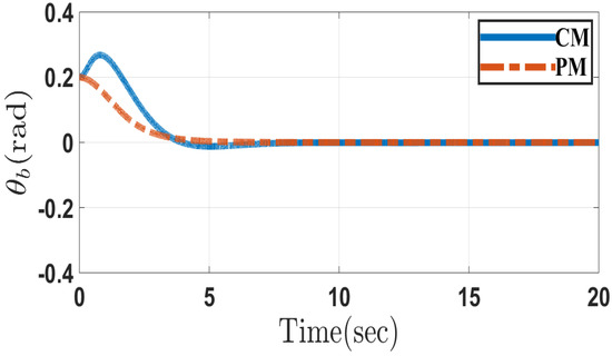
Figure 2. Pitch angle of the system in the conventional method (CM) and proposed method (PM) in Case 1.

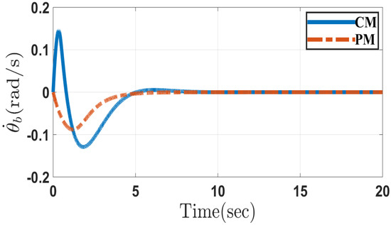
Figure 3. Pitch angular velocity of the system in the conventional method (CM) and the proposed method (PM) in Case 1.

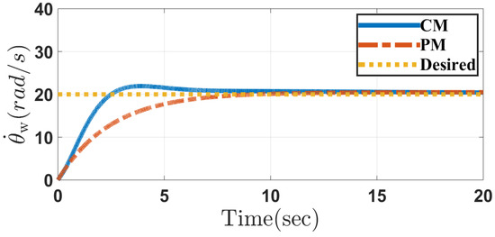
Figure 4. Wheel angular velocity of the system in the conventional method (CM) and the proposed method (PM) in Case 1.

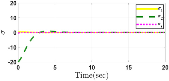
Figure 5. Sliding mode surfaces in the conventional method in Case 1.

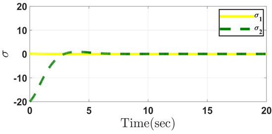
Figure 6. Sliding mode surfaces in the proposed method in Case 1.

Figure 7 depicts the input torque of wheels in Case 1 through the conventional and the proposed methods, respectively. It can be seen that they are similar to each other. However, as shown in Figure 8, the required power in the proposed method is much smaller than that required in the conventional method. There are high-frequency components in the input torque and power trajectories which are mainly due to the switching actions near the sliding surfaces in both the controllers. Though the QSMC controller is designed to smooth out the high-frequency components in the system outputs, it cannot eliminate them. On the other hand, the additional movable mechanism used in the proposed method increases the complexity of the system dynamics which also contributes to the high-frequency components.

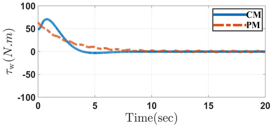
Figure 7. Input torque of wheels in the conventional method (CM) and the proposed method (PM) in Case 1.

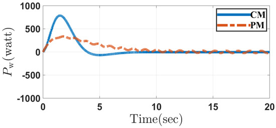
Figure 8. Input power of wheels in the conventional method (CM) and the proposed method (PM) in Case 1.

As shown in Figure 9 and Figure 10, the input torque and power required for the motion of the pendulum is almost negligible. As shown in Figure 11, the range of the angular displacement of the pendulum is very small. This shows that it can be made compact and be operated in a small space to achieve the control objectives without causing large disturbances to the system including the rider.

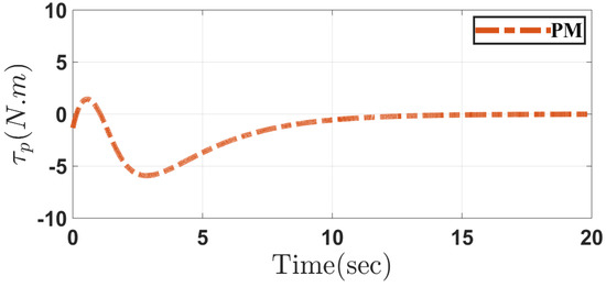
Figure 9. Input torque of movable mechanism in the proposed method (PM) in Case 1.

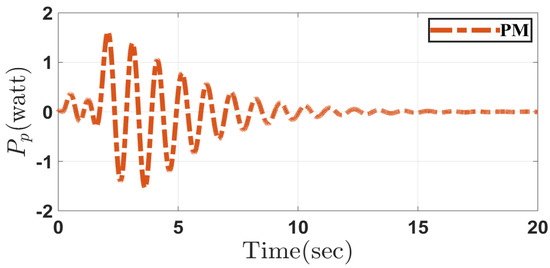
Figure 10. Input power of movable mechanism in the proposed method (PM) in Case 1.

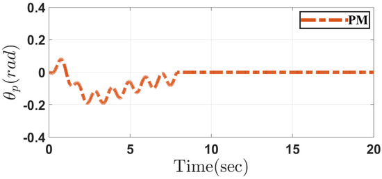
Figure 11. Movable mechanism angle in the proposed method (PM) in Case 1.

5.2. Case 2

In Case 2, the initial values of system are chosen as

$${\theta }_{b_0}=0.1rad,{\dot{\theta }}_{b_0}=0,{\theta }_{{\mathrm{w}}_0}=0,{\dot{\theta }}_{{\mathrm{w}}_0}=0,{\theta }_{p_0}=0,{\dot{\theta }}_{p_0}=0.$$

The control objectives are set as

$${\theta }_{b_d}=0,{\dot{\theta }}_{b_d}=0,{\dot{\theta }}_{{\mathrm{w}}_d}=10rad/s.$$

The control parameters for the HSMC and QSMC controllers are chosen same as the values selected in Case 1. As the mass of rider varies for each person, the uncertainty of the body’s mass should be considered to prove the robustness of the controllers. In this case, the uncertainty of body’s mass is chosen as $\Delta m_b=20kg$.

Figure 12, Figure 13, Figure 14, Figure 15, Figure 16, Figure 17, Figure 18, Figure 19, Figure 20 and Figure 21 depict the performance of system in Case 2 through the conventional and proposed methods. It can be seen that the results are similar to those obtained in Case 1. Considering the disturbances caused by parameter uncertainty, the system can overcome it and prove the controller robustness designed for both the methods.

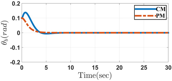
Figure 12. Pitch angle of system in the conventional method (CM) and the proposed method (PM) in Case 2.

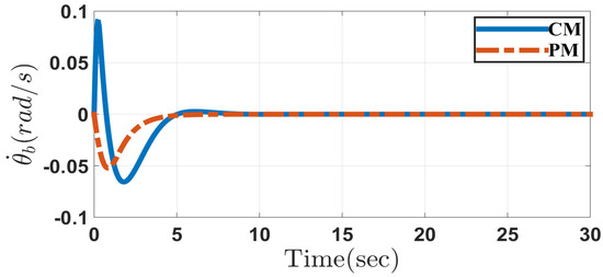
Figure 13. Pitch angular velocity of the system in the conventional method (CM) and the proposed method (PM) in Case 2.

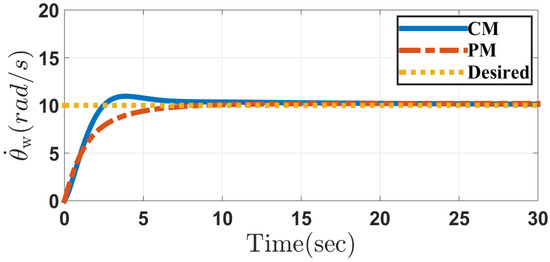
Figure 14. Wheel angular velocity of the system in the conventional method (CM) and the proposed method (PM) in Case 2.

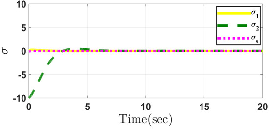
Figure 15. Sliding mode surfaces in the conventional method in Case 2.

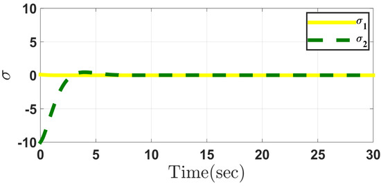
Figure 16. Sliding mode surfaces in the proposed method in Case 2.

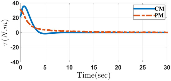
Figure 17. Input torque of the wheels in the conventional method (CM) and the proposed method (PM) in Case 2.

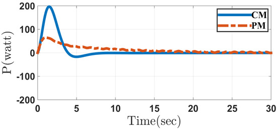
Figure 18. Input power of the wheels in the conventional method (CM) and the proposed method (PM) in Case 2.

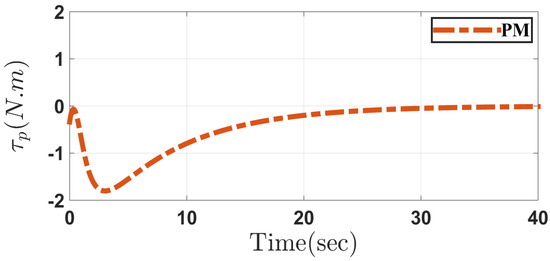
Figure 19. Input torque of the movable mechanism in the proposed method (PM) in Case 2.

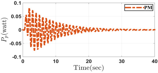
Figure 20. Input power of the movable mechanism in the proposed method (PM) in Case 2.

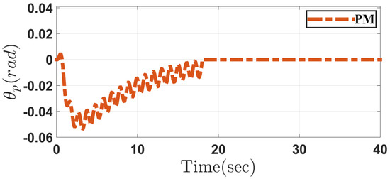
Figure 21. Movable mechanism angle in the proposed method (PM) in Case 2.

6. Conclusions

This paper presents a novel method for stability and velocity control of a two-wheeled robotic wheelchair. In this method, a movable pendulum-like movable mechanism is added to the wheelchair mainly for stability control. The Euler-Lagrange equation is used to establish the equation of motion of the system and a quasi-sliding mode control scheme is used in the controller design. The simulation results show that the proposed method achieves better stability and velocity control with less input power than the conventional methods only relying on the motions of the wheels. It is also robust against external disturbances. The future work is to implement the proposed method on a two-wheeled robotic wheelchair system under development in our lab.

References

- Stout, G. Some aspects of high performance indoor/outdoor wheelchairs. Bull. Prosthet Res. 1979, 16, 135–175. [Google Scholar] [PubMed]
- Abdulghani, M.M.; Al-Aubidy, K.M.; Ali, M.M.; Hamarsheh, Q.J. Wheelchair Neuro Fuzzy Control and Tracking System Based on Voice Recognition. Sensors 2020, 20, 2872. [Google Scholar] [CrossRef] [PubMed]
- Ren, T.J.; Chen, T.C. Modelling and control of a power-assisted mobile vehicle based on torque observer. IET Control Theory Appl. 2007, 1, 1405–1412. [Google Scholar] [CrossRef]
- Seki, H.; Sugimoto, T.; Tadakuma, S. Novel straight road driving control of power assisted wheelchair based on disturbance estimation and minimum jerk control. In Proceedings of the 2005 Conference Record of the Industry Applications, Fourtieth IAS Annual Meeting, Hong Kong, China, 2–6 October 2005; pp. 1711–1717. [Google Scholar]
- Almeshal, A.M.; Goher, K.M.; Nasir, A.N.K.; Tokhi, M.O. Steering and dynamic performance of a new configuration of a wheelchair on two wheels in various indoor and outdoor environments. In Proceedings of the 2013 18th International Conference on Methods & Models in Automation & Robotics, MMAR, Miedzyzdroje, Poland, 26–29 August 2013; pp. 223–228. [Google Scholar]
- Zhou, Y.; Wang, Z.; Chung, K.W. Turning Motion Control Design of a Two-Wheeled Inverted Pendulum Using Curvature Tracking and Optimal Control Theory. J. Optim. Theory Appl. 2019, 181, 634–652. [Google Scholar] [CrossRef]
- Wieczorek, B.; Warguła, Ł.; Rybarczyk, D. Impact of a hybrid assisted wheelchair propulsion system on motion kinematics during climbing up a slope. Appl. Sci. 2020, 10, 1025. [Google Scholar] [CrossRef]
- Hirata, K.; Murakami, T. Stability analysis of disturbance observer based controllers for two-wheel wheelchair systems. Adv. Robot. 2014, 28, 467–477. [Google Scholar] [CrossRef]
- Vermeiren, L.; Dequidt, A.; Guerra, T.M.; Rago-Tirmant, H.; Parent, M. Modeling, control and experimental verification on a two-wheeled vehicle with free inclination: An urban transportation system. Control Eng. Pract. 2011, 19, 744–756. [Google Scholar] [CrossRef]
- Han, J.; Li, X.; Qin, Q. Design of two-wheeled self-balancing robot based on sensor fusion algorithm. Int. J. Autom. Technol. 2014, 8, 216–221. [Google Scholar] [CrossRef]
- Cooper, R.A.; Boninger, M.L.; Cooper, R.; Kelleher, A. Use of the INDEPENDENCE 3000 IBOT™ transporter at home and in the community: A case report. Disabil. Rehabil. Assist. Technol. 2006, 1, 111–117. [Google Scholar] [CrossRef]
- Arthanat, S.; Desmarais, J.M.; Eikelberg, P. Consumer perspectives on the usability and value of the iBOT® wheelchair: Findings from a case series. Disabil. Rehabil. Assist. Technol. 2012, 7, 153–167. [Google Scholar] [CrossRef] [PubMed]
- Uustal, H.; Minkel, J.L. Study of the Independence IBOT 3000 Mobility System: An innovative power mobility device, during use in community environments. Arch. Phys. Med. Rehabil. 2004, 85, 2002–2010. [Google Scholar] [CrossRef]
- Baloh, M.; Parent, M. Modeling and model verification of an intelligent self-balancing two-wheeled vehicle for an autonomous urban transportation system. In Proceedings of the Conference on Computational Intelligence, Robotics, and Autonomous Systems, Singapore, 15 December 2003; pp. 1–7. [Google Scholar]
- Karkoub, M.A.; Parent, M. Modelling and non-linear feedback stabilization of a two-wheel vehicle. Proc. Inst. Mech. Eng. Part J. Syst. Control Eng. 2004, 218, 675–686. [Google Scholar] [CrossRef]
- Ghaffari, A.; Shariati, A.; Shamekhi, A.H. A modified dynamical formulation for two-wheeled self-balancing robots. Nonlinear Dyn. 2016, 83, 217–230. [Google Scholar] [CrossRef]
- Nikpour, M.; Huang, L.; Al-Jumaily, A.M.; Lotfi, B. Stability control of mobile inverted pendulum through an added movable mechanism. In Proceedings of the 25th International Conference on Mechatronics and Machine Vision in Practice, M2VIP, Stuttgart, Germany, 20–22 November 2018; pp. 1–6. [Google Scholar]
- Raffo, G.V.; Ortega, M.G.; Madero, V.; Rubio, F.R. Two-wheeled self-balanced pendulum workspace improvement via underactuated robust nonlinear control. Control Eng. Pract. 2015, 44, 231–242. [Google Scholar] [CrossRef]
- Ahmad, N.S. Robust H∞-Fuzzy Logic Control for Enhanced Tracking Performance of a Wheeled Mobile Robot in the Presence of Uncertain Nonlinear Perturbations. Sensors 2020, 20, 3673. [Google Scholar] [CrossRef]
- Raffo, G.V.; Madero, V.; Ortega, M.G. An application of the underactuated nonlinear H∞ controller to two-wheeled self-balanced vehicles. In Proceedings of the IEEE 15th Conference on Emerging Technologies & Factory Automation, ETFA, Bilbao, Spain, 13–16 September 2010; pp. 1–6. [Google Scholar]
- Shen, H.; Iorio, J.; Li, N. Sliding Mode Control in Backstepping Framework for a Class of Nonlinear Systems. J. Mar. Sci. Eng. 2019, 7, 452. [Google Scholar] [CrossRef]
- Hong, G.S.; Yu, D.; Wong, Y.S. Integral sliding mode control for fast tool servo diamond turning of micro-structured surfaces. Int. J. Autom. Technol. 2011, 5, 4–10. [Google Scholar]
- Nikpour, M.; Huang, L.; Al-Jumaily, A.M. Stability and Direction Control of a Two-Wheeled Robotic Wheelchair Through a Movable Mechanism. IEEE Access 2020, 8, 45221–45230. [Google Scholar] [CrossRef]
- Elmokadem, T.; Zribi, M.; Youcef-Toumi, K. Control for Dynamic Positioning and Way-point Tracking of Underactuated Autonomous Underwater Vehicles Using Sliding Mode Control. J. Intell. Robot. Syst. 2019, 95, 1113–1132. [Google Scholar] [CrossRef]
- Yue, M.; Wei, X. Dynamic balance and motion control for wheeled inverted pendulum vehicle via hierarchical sliding mode approach. Proc. Inst. Mech. Eng. Part J. Syst. Control Eng. 2014, 228, 351–358. [Google Scholar] [CrossRef]
- Huang, J.; Guan, Z.H.; Matsuno, T.; Fukuda, T.; Sekiyama, K. Sliding-mode velocity control of mobile-wheeled inverted-pendulum systems. IEEE Trans. Robot. 2010, 26, 750–758. [Google Scholar] [CrossRef]
- Huang, J.; Ding, F.; Fukuda, T.; Matsuno, T. Modeling and velocity control for a novel narrow vehicle based on mobile wheeled inverted pendulum. IEEE Trans. Control Syst. Technol. 2013, 21, 1607–1617. [Google Scholar] [CrossRef]
- Sago, Y.; Noda, Y.; Kakihara, K.; Terashima, K. Parallel two-wheel vehicle with underslung vehicle body. Mech. Eng. J. 2014, 1, 1–12. [Google Scholar] [CrossRef][Green Version]
- Sago, Y.; Terashima, K.; Noda, Y.; Kakihara, K. Attitude control using active-mass-system in parallel two-wheel vehicle with underslung vehicle body. In Proceedings of the 2014 IEEE International Conference on Systems, Man, and Cybernetics, SMC, San Diego, CA, USA, 5–8 October 2014; pp. 1532–1537. [Google Scholar]
- Rao, S.S.; Yap, F.F. Mechanical Vibrations; Prentice Hall: Upper Saddle River, NJ, USA, 2011; Volume 4. [Google Scholar]
- Craig, J.J. Introduction to Robotics: Mechanics and Control; Pearson Education: Bengaluru, India, 2009; Volume 3/E. [Google Scholar]
- Bolton, W. Mechatronics: Electronic Control Systems in Mechanical and Electrical Engineering; Pearson Education: London, UK, 2003. [Google Scholar]
- Shtessel, Y.; Edwards, C.; Fridman, L.; Levant, A. Sliding Mode Control and Observation; Springer: New York, NY, USA, 2014. [Google Scholar]
- Qian, D.; Yi, J. Hierarchical Sliding Mode Control for Under-Actuated Cranes; Springer: Heidelberg/Berlin, Germany, 2016. [Google Scholar]
© 2020 by the authors. Licensee MDPI, Basel, Switzerland. This article is an open access article distributed under the terms and conditions of the Creative Commons Attribution (CC BY) license (http://creativecommons.org/licenses/by/4.0/).