Characteristics of Position and Pressure Control of Separating Metering Electro-Hydraulic Servo System with Varying Supply Pressure for Rolling Shear

Featured Application

To improve energy efficiency while also ensuring position tracking accuracy, this paper gives the design and the analysis of a separate metering electro-hydraulic servo system with varying supply pressure for a rolling shear. This work is also suitable for similar engineering applications.

Abstract

The traditional valve-controlled hydraulic servo system has large throttling losses and undergoes serious heat problems when used in electro-hydraulic servo systems (EHSSs) for a rolling shear. In order to improve the energy efficiency of the EHSS for the rolling shear while also ensuring the position tracking accuracy, the separate metering electro-hydraulic servo system with varying supply pressure (VSP-SMEHSS) is proposed in this work. The inlet valve controls the position of a hydraulic cylinder, while the outlet valve controls the back pressure of the hydraulic cylinder. However, due to the disturbance caused by the varying supply pressure, the proportional–integral–derivative (PID) controller or active disturbance rejection controller (ADRC) cannot meet the requirements of accuracy. In order to solve this problem, based on a nonlinear disturbance observer (NDO) and a tracking differentiator (TD), a dynamic surface control (DSC) is proposed in this work. Firstly, the stability of the controller is validated using the Lyapunov method. Then, experiments are conducted to verify the proposed control strategy. As a result, the hydraulic cylinder can accurately track the reference displacement signal and effectively reduce the pressure drop at the valve’s orifice, due to which the hydraulic system achieves significant energy-savings. Compared with that of the EHSS, the energy consumption of the VSP-SMEHSS is reduced by 44.6%.

1. Introduction

A hydraulic roller shear is used to cut steel plates into a certain size on a rolling production line. When the rolling shear is driven by two hydraulic cylinders, an upper blade is rapidly rolling on the steel plate to cut it. If the trajectory of the upper blade is inaccurate, it will affect the quality of the shear section of the steel plate. Therefore, the trajectories of the hydraulic cylinders need to be precisely controlled for better quality. However, the traditional four-sided spool-valve-controlled system undergoes significant throttling losses [1,2,3,4], which generates a lot of heat and affects the reliability of the system. High temperature during the process affects the control of the system. Therefore, improving the energy efficiency of the electro-hydraulic servo system (EHSS) while guaranteeing the tracking accuracy is a topic worth research attention.

In order to reduce throttling losses of a valve-controlled hydraulic servo system, one solution is to use a closed pump-controlled system [5,6,7,8], which includes a fixed-displacement pump system driven by a servo motor and a constant-speed variable-displacement pump system [9,10]. The flow rate of the pump is varied to control the speed of an actuator. Due to this reason, theoretically speaking, there are no throttling losses. Due to obvious energy-saving effects, this technology has been applied to hydraulic systems of plastic injection molding machines [11]. However, this scheme has a poor dynamic response, and it is difficult to meet the high-response requirement of a rolling shear EHSS.

Load-sensing technology is another solution to reduce throttling losses [12,13], and it is widely used in hydraulic systems of excavators [14] and steering systems of hydraulic power [15]. In the load-sensing system, the pressure of the pump changes with the change in load force. The output flow of the pump matches the speed of the actuator. However, the dynamic response of this scheme is still poor, which is also not suitable for rolling shear EHSSs.

Another solution for reducing throttling losses is a separate metering system [16,17]. In the literature [18] based on separate metering systems, segmented speed and continuous displacement control strategies were proposed. These studies showed that the energy efficiency of a hydraulic system using the separate metering technology was improved. In a previous work [19], a three-level coordinated control method was proposed for a load-port-independent system. Compared to that in the conventional valve control system, throttling losses were significantly reduced. In another study [20], four control strategies were proposed for a separate metering system to control the boom hydraulic cylinder of an excavator. The control performance and the energy efficiency of the system were improved. In a previous work [21] based on a separate metering system, a pump-and-valve cooperative control strategy was proposed to improve the energy efficiency of the system. A previous study [22] showed that two proportional directional valves can be used to control hydraulic cylinders. Among them, one was used for controlling the speed of the hydraulic cylinders, while the other was used for controlling the back pressures of the hydraulic cylinders. In two other studies [23,24], four valves were used to control the speed of a hydraulic cylinder. Since the four valves were independent, the system had more degrees of freedom. In another study [25], a programmable valve with five 2/2-way high-speed on–off valves was studied. The adaptive robust control strategy was applied to control the speed of a hydraulic cylinder and the system pressure. In another work [26], a separate metering system was used for controlling the position of the press, and based on an extended segmented disturbance observer, a nonlinear motion controller was proposed. Under the influence of an unknown load force, the press obtained excellent motion tracking performance. However, the energy-saving characteristics of the system were not considered in the work.

In a separate metering system, there are no mechanical connections between valve metering orifices, whereas the system layout is flexible and convenient. Therefore, based on the independent system of a load port and considering the fast response, high precision, and the requirement for low throttling losses for a rolling shear hydraulic servo system, a separate metering electro-hydraulic servo system with variable supply pressure (VSP-SMEHSS) was proposed. Because the supply pressure matches the load force, the pressure drops across the valves’ orifices are reduced. This, in turn, helps in achieving energy-savings. However, varying supply pressure brings disturbance to the system, which results in difficulties in the design of a controller.

In order to solve the disturbance caused by the varying supply pressure, based on dynamic surface control (DSC) methods, a DSC method with a tracking differentiator (TD) and a nonlinear disturbance observer (NDO) was proposed in this paper. The NDO was used to eliminate the disturbance caused by the varying supply pressure in the system. In addition, a first-order filter in the DSC was replaced by the TD, which improved the performance of the controller.

In Section 2 of the paper, a VSP-SMEHSS is proposed and modeled. In Section 3, the design of a supply pressure regulator (SPR) is presented. Then, the positions and pressures of controllers are designed using the DSC method combined with both the TD and the NDO. In Section 4, experimental results are presented to show the effectiveness of the proposed control method and the feasibility of the energy-saving aspect of the proposed control method. Based upon the results, conclusions are drawn and presented in Section 5.

2. Working Principle of a Rolling Shear and Schematic of an Electro-Hydraulic Servo System

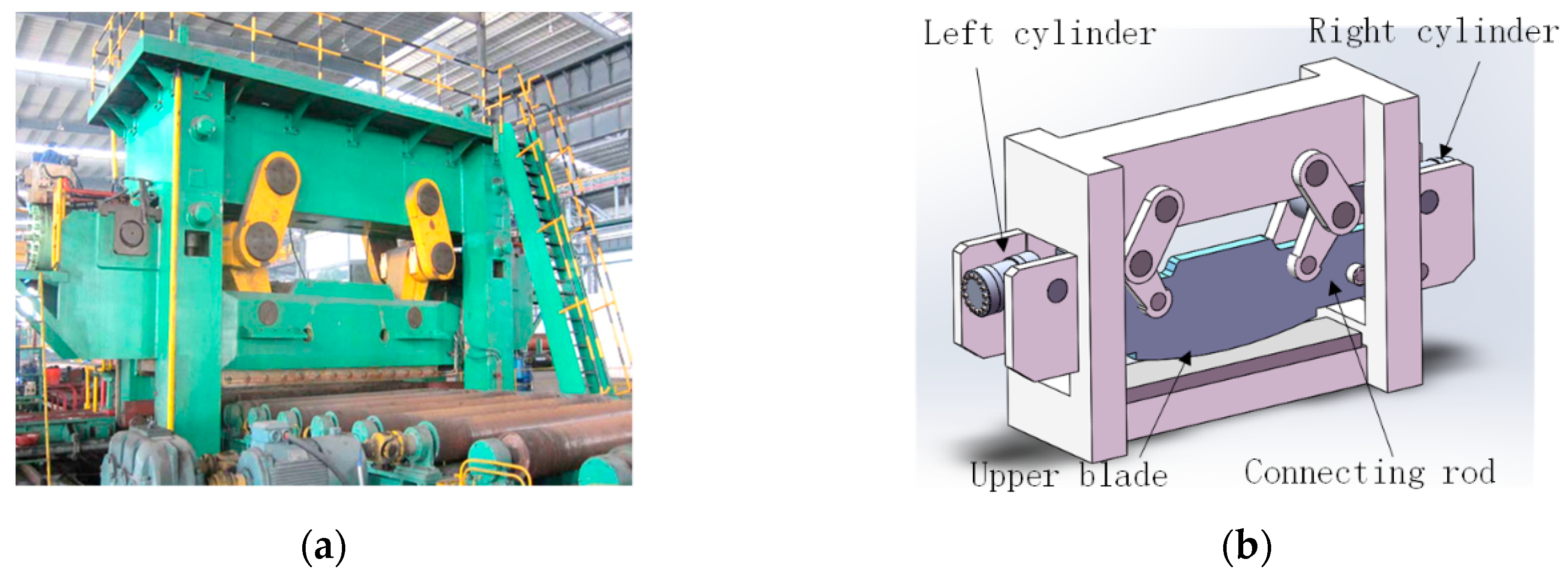
2.1. Working Principle of a Rolling Shear

A hydraulic rolling shear is a device used for shearing steel plates in rolling production lines. It is mainly composed of an upper blade, connecting rods and two hydraulic cylinders (Figure 1). Figure 2 illustrates the work cycle of a rolling shear. The two hydraulic cylinders push the connecting rods to drive the upper cutting edge to perform the rolling motion. At the beginning of the work cycle, the hydraulic cylinders on both sides are retracted, while the upper blade is at the highest position (Figure 2a). Then, the left-hand hydraulic cylinder extends, and the upper blade descends to start cutting a steel plate (Figure 2b). When cutting, the hydraulic cylinders on both sides harmoniously drive the upper blade to create the rolling motion on the steel plate (Figure 2c). When the cutting finishes, the right-hand hydraulic cylinder retracts, whereas the upper blade is lifted up to prepare for the next work cycle (Figure 2d). Figure 3 shows the position curves of the two hydraulic cylinders during one work cycle.

2.2. Electro-Hydraulic Servo System

The schematic of the proposed VSP-SMEHSS is shown in Figure 4. The proposed system consists of two hydraulic cylinders, four servo valves, two servo-hydraulic pumps, and two relief valves. The two hydraulic cylinders work in the same way. The inlets and the outlets of the cylinders are driven by two separate servo valves. A relief valve is used to ensure that the system pressure does not exceed the maximum allowable pressure. For the left-hand hydraulic cylinder, shown in Figure 4, the hydraulic system contains two control loops. One is the displacement closed loop at the inlet, which is used to control the trajectory of the hydraulic cylinder using valve 1. This helps in accurately following a given signal. The other is the pressure closed loop. The back pressure should be controlled accurately, and the control loop needs a fast dynamic response. Therefore, valve 2 is utilized rather than a proportional relief valve. A variable pump is used to provide pressure for the entire system, whereas the pressure is proportional to an input signal. The supply pressure changes with the change in load force, which reduces the pressure drop of a valve’s orifice. Due to this reason, the system’s energy consumption is reduced.

3. Electro-Hydraulic Servo System Modeling

In order to derive the control law, the EHSS must be modeled. For the system shown in Figure 4, the two cylinders are controlled in the same way. The control system on the left-hand side (shown in Figure 4) is modeled. This system can be divided into two subsystems, namely the position servo system at the inlet and the pressure servo system at the outlet. The two subsystems are modeled as follows.

3.1. Modeling of the Position Servo System

In the position control loop, a servo valve is used to control the trajectory of the hydraulic cylinder $x_L$ to follow a given signal $x_d$. The force on the hydraulic cylinder can be given using Equation (1):

$${\ddot{x}}_L=\frac{1}{m}(p_1{A}_1-p_2{A}_2-b{\dot{x}}_L-f_L)+\Delta e_2,$$

(1)

where $m$ is the total mass of the piston, $f_L$ is the load force, which is related to the thickness and the material of the steel plate and the shear speed and time, $b$ is the viscous damping coefficient and $\Delta e_2$ is the uncertainty due to parameter perturbation, modeling errors, and disturbances. Since the natural frequency of the valve is much higher than the natural frequency of the system, the valve’s dynamics can be regarded as a proportional component. The relationship between the spool displacement and the input signal is given by Equation (2):

$$x_{v1}=k_{s1}{u}_1,$$

(2)

where $x_{v1}$ is the spool’s displacement, $k_{s1}$ is the valve gain and $u_1$ is the signal input to the valves; $q_1$ represents the flow at the inlet, which is related to the opening of the valve orifice $x_{v1}$ and the pressure drop $\Delta p_1$ [27], and is obtained using Equation (3):

$$q_1=k_{v1}{x}_{v1}\sqrt{\Delta p_1},$$

(3)

where $k_{v1}$ is the flow coefficient and $\Delta p_1$ is the pressure drop of the valve, which is given by Equation (4):

$$\Delta p_1=\{\begin{array}{l}{p}_s-p_1,{\mathrm{x}}_{v1}\ge 0\\ p_1-p_o,{\mathrm{x}}_{v1}<0\end{array},$$

(4)

where $p_s$ is the supply pressure and $p_o$ is the tank pressure.

For the chamber at the inlet, according to the flow continuity equation, Equation (5) is obtained and shown as following:

$${\dot{p}}_1=[q_1-A_1{\dot{x}}_L-C_{ep1}{p}_1-C_{ip1}(p_1-p_2)]\frac{{\beta }_e}{V_1+A_1{x}_L}+\Delta e_3,$$

(5)

where ${\beta }_e$ is the effective oil bulk modulus, $p_1$ is the pressure of the piston chamber, $p_2$ is the pressure of the rod chamber, $A_1$ is the area of the piston, $A_2$ is the effective area of the rod, $x_L$ is the displacement of the rod, $V_1$ and $V_2$ are the initial volumes of the cylinder chambers, including the chamber volume of the connected pipeline, $C_{ep1}$ is the external leakage coefficient, $C_{ip1}$ is the internal leakage coefficient and $\Delta e_3$ is a variable arising from parameter perturbation, modeling errors, and disturbance.

Considering that $u_1$ is the system input and $x_L$ is the system output, the system state variable is defined using Equation (6):

$$x_i={[x_{i1},x_{i2},x_{i3}]}^T={[x_L,{\dot{x}}_L,p_1]}^T.$$

(6)

According to Equations (1)–(5), the model of the position servo system can be illustrated using Equation (7):

$$\{\begin{array}{l}{\dot{x}}_{i1}=x_{i2}\\ {\dot{x}}_{i2}=c_1{x}_{i3}+c_2{x}_{i2}+{\delta }_{i2}+{\theta }_{i2}\\ {\dot{x}}_{i3}=c_3{u}_1+c_4{x}_{i2}+{\theta }_{i3}\end{array},$$

(7)

where ${\delta }_{i2}=\frac{-p_2{A}_2-f_L}{m}$, $c_1=\frac{A_1}{m}$, $c_2=-\frac{b}{m}$, $c_3=\frac{{\beta }_e}{V_1}{k}_{v1}{k}_{s1}\sqrt{\Delta p_1}$, $c_4=-\frac{{\beta }_e}{V_1}{A}_1$ and ${\theta }_{i2}$ and ${\theta }_{i3}$ are the uncertainties due to modeling errors, parameter uncertainties, and disturbance caused by the varying supply pressure. An NDO is designed to compensate for ${\theta }_{i2}$ and ${\theta }_{i3}$ (as explained in Section 4).

3.2. Modeling of the Pressure Servo System

In the pressure control loop, a servo valve is used to regulate the cylinder’s back pressure for a given signal. Similarly, the valve’s dynamics is regarded as a proportional component. The relationship between the displacement of the spool and the input signal can be expressed as follows:

$$x_{v2}=k_{s2}{u}_2.$$

(8)

Since the natural frequency of the valve is much higher than the natural frequency of the system, the relationship between the spool displacement and the input signal is represented using Equation (9):

$$x_{v2}=k_{s2}{u}_2,$$

(9)

where $x_{v2}$ is the spool’s displacement, $k_{s2}$ is the valve’s gain and $u_2$ is the signal input to the valves. The flow at the outlet $q_2$, which is related to the opening of the valve’s orifice $x_{v2}$, is given by Equation (10):

$$q_2=k_{v2}{x}_{v2}\sqrt{\Delta p_2}$$

(10)

where $k_{v2}$ is the flow coefficient, and $\Delta p_2$ is the pressure drop of the valve [27], which is given by Equation (11):

$$\Delta p_2=\{\begin{array}{l}{p}_s-p_2,{\mathrm{x}}_{v2}\ge 0\\ p_2-p_o,{\mathrm{x}}_{v2}<0\end{array}.$$

(11)

For the chamber at the outlet, according to the flow continuity equation, Equation (12) is obtained and shown as following:

$${\dot{p}}_2=[q_2+A_2{\dot{x}}_L-C_{ep1}{p}_2+C_{ip2}(p_1-p_2)]\frac{{\beta }_e}{V_2-A_2{x}_L}+\Delta e_1,$$

(12)

where ${\beta }_e$ is the effective oil bulk modulus, $p_2$ is the pressure of the rod chamber, $A_2$ is the effective area of the rod, $x_L$ is the displacement of the rod, $V_2$ is the initial volume of the cylinder chamber, $C_{ep2}$ is the external leakage coefficient, $C_{ip2}$ is the internal leakage coefficient and $\Delta e_1$ is the uncertainty due to parameter perturbation, modeling errors, and disturbance.

Considering that $u_2$ is the system input and $p_2$ is the system output, according to Equations (9)–(12), the state space equation of the system can be written as Equation (13):

$${\dot{x}}_{o1}=d_1{u}_2+d_2+{\theta }_{o1},$$

(13)

where $x_{o1}$ is the state variable, $d_1=\frac{{\beta }_e}{V_2-A_2{x}_L}{k}_{v2}{k}_{s2}\sqrt{\Delta p_2}$, $d_2=\frac{{\beta }_e}{V_2-A_2{x}_L}{A}_2{\dot{x}}_L$, and ${\theta }_{o1}$ is the uncertainty due to modeling error, parameter uncertainties, and disturbance. Similarly, an NDO is designed to compensate for ${\theta }_{o1}$.

4. Design of the Controller

As shown in Figure 5, the controller consists of an SPR, a position controller, and a cylinder pressure controller. The SPR adjusts the system’s supply pressure according to the magnitude of a load force. Due to this reason, the system pressure matches the load force, thereby reducing the throttling losses of valves’ orifices and achieving energy-saving effects. The position controller is used to control the displacement of the cylinder to follow a given motion signal, thus ensuring that the upper blade of the rolling shear is accurately moving according to the trajectory. The pressure controller is used to regulate the pressure in the cylinder chamber near a reference signal.

4.1. Supply Pressure Regulator

Generally, the supply pressure of an EHSS remains constant and is often set to a large value to ensure that the system produces sufficient force. Since the inlet and the outlet of a hydraulic cylinder are controlled by the same spool when the load force is small, the supply pressure results in a large pressure drop at a valve’s orifice and increases the system temperature.

The VSP-SMEHSS proposed in this paper breaks the mechanical connection between the inlet and the outlet, whereas the supply pressure changes with the change in load. When the load force is small, the supply pressure becomes small, due to which the pressure drop at a valve’s orifice decreases. Since the back pressure of the hydraulic cylinder can be controlled separately, the back pressure is set to a smaller value to reduce throttling losses of the outlet orifice, thus achieving energy-saving effects.

In this paper, an electro-hydraulic proportional variable pump was used as a hydraulic source. The output pressure of the variable pump is proportional to the input signal. Considering the hysteresis characteristics of the variable pump, the output pressure can be expressed using Equation (14):

$$p_{pump}(t)=k_p\cdot u_p(t-t_0),$$

(14)

where $p_{pump}$ is the output pressure, $u_p$ is the input signal and $t_0$ is the response time of the variable pump. For the position servo system, the minimum required pressure $p_{s1}$ is given by Equation (15):

$$p_{s1}=\frac{f_L+{\lambda }_f}{A_1}+\frac{A_2}{A_1}{p}_2+\Delta P_{v1}+\Delta P_1,$$

(15)

where $f_L$ is the load force, $p_2$ is the back pressure, $\Delta P_1$ is the adjustment margin and $\Delta P_{v1}$ is the pressure drop across the valve’s orifice.

For the pressure servo system, the required minimum supply pressure $p_s$ is given by Equation (16):

$$p_{s2}=P_d+\Delta P_{v2}+\Delta P_2,$$

(16)

where $P_d$ is the reference signal and $\Delta P_2$ is the adjustment margin. Therefore, the control law of an oil SPR is expressed using Equation (17):

$$u_3(t)=k_p\cdot max\{p_{s1}(t+t_0),p_{s2}\}.$$

(17)

It should be noted that the maximum acceleration of the load is given by Equation (18):

$$a=A_1\Delta P_1/m.$$

(18)

According to Equation (18), it is known that a larger $\Delta P_1$ can generate a larger acceleration, which means that the load can quickly track the command signal. However, a large $\Delta P_1$ will result in a higher $p_{s1}$, which means that the system will generate a larger throttling loss. Similarly, a larger $\Delta P_2$ results in a higher $p_{s2}$. Therefore, the choices of $\Delta P_1$ and $\Delta P_2$ requires a trade-off between the system dynamics and the energy-saving effects.

4.2. Design of the Position Controller

Many researchers have studied control algorithms for EHSSs. In a previous study [28], a two-loop control structure of a position–pressure master-slave controller in a rolling shear hydraulic system was studied. However, the nonlinear characteristics of the system were not considered in the design process of the controller. The DSC algorithm can handle nonlinear problems [29,30,31,32]. However, a first-order filter used in the DSC limits the performance of the controller. In this section (Section 4.2), based on NDO and TDDSC control methods, a position controller was designed. An NDO was used to observe the disturbance in the system. The first-order filter of the NDO was replaced by a TD, which has a better performance than the first-order filter used in the DSC [33]. The TD used in this paper is expressed using Equation (19):

$$\{\begin{array}{l}{\dot{x}}_1=x_2\\ {\dot{x}}_2=R^2\{-a_1\arctan (f_1(x_1-v)-a_2\arctan (\frac{f_2{x}_2}{R})\}\end{array},$$

(19)

where $v$ is the input, $x_1$ is the tracking output of $v$ and $x_2$ is the tracking output of the derivation of $v$; $R$, $a_1$, and $f_1$ are the gain of TD, and they are positive, which determine the tracking speed of TD; $a_2$ and $f_2$ determine the differentiation effect of the TD. The detailed parameter-tuning method was described in the literature [33].

The design of the position controller is divided into three steps using the TDDSC method. In this paper, symbol $^$ represents the estimate of a variable, symbol $˜$ represents the estimate error of a variable. For example, $A$ is a variable, $\widehat{A}$ is used to denote the estimate of $A$, whereas $\tilde{A}$ is used to represent the error in the estimate of $A$, which means the relationship: $\tilde{A}=A-\widehat{A}$. The error state variables are defined using Equation (20):

$$\{\begin{array}{l}{e}_1=x_{i1}-x_d\\ e_2=x_{i2}-{\alpha }_1\\ e_3=x_{i3}-{\alpha }_2\end{array},$$

(20)

where ${\alpha }_1$ and ${\alpha }_2$ are the virtual control variables.

Step 1:

The first error surface $e_1$ is defined using Equation (21):

$$e_1=x_{i1}-x_d.$$

(21)

The derivative of Equation (21) is given by Equation (22):

$${\dot{e}}_1={\dot{x}}_{i1}-{\dot{x}}_d=x_{i2}-{\dot{x}}_d.$$

(22)

Furthermore, the virtual control variable ${\alpha }_1$ is given by Equation (23):

$${\alpha }_1=-k_1{e}_1+{\dot{x}}_d,$$

(23)

where $k_1$ is the controller gain and $k_1>0$.

When the Lyapunov function is expressed as $V_1=\frac{1}{2}{e}_1^2$, Equation (24) is obtained and shown as following:

$${\dot{V}}_1=e_1{\dot{e}}_1=e_1(e_2+{\alpha }_1-{\dot{x}}_d)=-k_1{e}_1^2+e_1{e}_2.$$

(24)

As long as $e_2$ converges to 0 and $k_1>0$, it can be guaranteed that ${\dot{V}}_1<0$. Therefore, step 2 is needed.

Step 2:

The second error surface $e_2$ is defined using Equation (25):

$$e_2=x_{i2}-{\alpha }_1.$$

(25)

The derivative of $e_2$ is given by Equation (26):

$${\dot{e}}_2={\dot{x}}_{i2}-{\dot{\alpha }}_1=c_1{x}_3+c_2{x}_{i2}+{\theta }_{i2}+{\delta }_2-{\dot{\alpha }}_1,$$

(26)

where ${\dot{\alpha }}_1$ is obtained using the TD, which is given by Equation (19). In order to estimate ${\theta }_{i2}$, the following NDO is designed (Equation (27)):

$$\{\begin{array}{l}{\widehat{\theta }}_{i2}={\sigma }_{i2}+{\eta }_{i2}{x}_{i2}\\ {\dot{\sigma }}_{i2}=-{\eta }_{i2}{\sigma }_{i2}-{\eta }_{i2}(c_1{x}_{i3}+c_2{x}_{i2}+{\delta }_{i2}+{\eta }_{i2}{x}_{i2})\end{array},$$

(27)

where ${\eta }_{i2}$ is the observer gain (${\eta }_{i2}>0$), which is related to the convergence speed of the NDO, and ${\sigma }_{i2}$ is the internal variable. Furthermore, the virtual control variable ${\alpha }_2$ is given by Equation (28):

$${\alpha }_2=\frac{1}{c_1}(-k_2{e}_2-c_2(e_2+{\alpha }_1)-{\widehat{\theta }}_{i2}-e_1-{\delta }_{i2}+{\widehat{\dot{\alpha }}}_1),$$

(28)

where $k_2$ is the controller gain, ${\widehat{\dot{\alpha }}}_1$ is obtained using TD and ${\widehat{\theta }}_{i2}$ is the observed uncertainty. When the Lyapunov function is described as $V_2=V_1+\frac{1}{2}{e}_2^2$, Equation (29) is obtained and shown as following:

$${\dot{V}}_2=-k_1{e}_1^2-k_2{e}_2^2+c_1{e}_2{e}_3+e_2{\tilde{\theta }}_{i2}-e_2{\tilde{\dot{\alpha }}}_1.$$

(29)

As long as $e_3$, ${\tilde{\theta }}_{i2}$, and ${\widehat{\dot{\alpha }}}_1$ converge to 0 and $k_2>0$, it can be guaranteed that ${\dot{V}}_2<0$. Therefore, step 3 is devised.

Step 3:

The second error surface $e_3$ is defined using Equation (30):

$$e_3=x_{i3}-{\alpha }_2.$$

(30)

The derivative of $e_3$ is given by Equation (31):

$${\dot{e}}_3={\dot{x}}_3-{\dot{\alpha }}_2=c_3{u}_1+c_4(e_2+{\alpha }_1)+{\theta }_{i3}-{\dot{\alpha }}_2.$$

(31)

The control law is obtained using Equation (32):

$$u_i=\frac{1}{c_3}(-k_3{e}_3-c_4(e_2+{\alpha }_1)-{\widehat{\theta }}_{i3}+{\widehat{\dot{\alpha }}}_2-c_1{e}_2),$$

(32)

where $k_3$ is the controller gain and $k_3>0$. Furthermore, ${\widehat{\dot{\alpha }}}_2$ is obtained using the TD given in Equation (19). ${\widehat{\theta }}_{i3}$ is obtained using the NDO (Equation (33)), shown as follows:

$$\{\begin{array}{l}{\widehat{\theta }}_{i3}={\sigma }_{i3}+{\eta }_{i3}{x}_{i3}\\ {\dot{\sigma }}_{i3}=-{\eta }_{i3}{\sigma }_{i3}-{\eta }_{i3}(c_3{x}_{i4}+c_4{x}_{i2}+{\eta }_{i3}{x}_{i3})\end{array},$$

(33)

where ${\eta }_{i3}$ is the observer gain (${\eta }_{i3}>0$), which is related to the convergence speed of the NDO, and ${\sigma }_{i3}$ is the internal variable.

4.3. Design of the Pressure Controller

The pressure controller is designed to control the cylinder outlet chamber pressure $p_2$ to follow a given signal $p_d$. Similarly, according to Equation (13), the control law is given by Equation (34):

$$u_o=(-d_2+{\dot{p}}_d-{\widehat{\theta }}_{o1}-k_{o}e)/d_1,$$

(34)

where $k$ is the controller gain,$d_1=\frac{{\beta }_e{K}_{v2}{K}_{s2}\sqrt{\Delta P_2}}{V_2-A_2{x}_L}$ and $d_2=\frac{A_2{\dot{x}}_L{\beta }_e}{V_2-A_2{x}_L}$; $e_o$ is the tracking error and is given by: $e_o=p_2-p_d$; ${\widehat{\theta }}_{o1}$ is the estimated uncertainty in the system, which is obtained using the NDO (Equation (35)):

$$\{\begin{array}{l}{\widehat{\theta }}_{o1}={\sigma }_{o1}+{\eta }_{o1}{x}_{o1}\\ {\dot{\sigma }}_{o1}=-{\eta }_{o1}{\sigma }_{o1}-{\eta }_{o1}(d_{1}u+d_2+{\eta }_{o1}{x}_{o1})\end{array},$$

(35)

where ${\eta }_{o1}$ is the observer gain (${\eta }_{o1}>0$), which is related to the convergence speed of the NDO, and ${\sigma }_{o1}$ is the internal variable.

4.4. Stability Analysis

In order to verify the stability and the convergence of the position controller, for the position servo system, the Lyapunov function is written as: $V_i=V_2+\frac{1}{2}{e}_3{}^2$, and results in Equation (36):

$${\dot{V}}_i=-k_1{e}_1^2-k_2{e}_2^2-k_3{e}_3^2+e_2{\tilde{\theta }}_{i2}+e_3{\tilde{\theta }}_{i3}-e_2{\tilde{\dot{\alpha }}}_1-e_3{\tilde{\dot{\alpha }}}_2.$$

(36)

Equation (37) shows the assumptions used here, and is written as:

$$\{\begin{array}{l}k=\min \{k_1,k_2,k_3\}\\ \epsilon =|{\tilde{\theta }}_{i2}|+|{\tilde{\theta }}_{i3}|+|{\tilde{\dot{\alpha }}}_1|+|{\tilde{\dot{\alpha }}}_2|\end{array},$$

(37)

Based on Equations (36) and (37), Equation (38) is expressed as:

$${\dot{V}}_i\le -k(e_1^2+e_2^2+e_3^2)+|e_2||{\tilde{\theta }}_2|+|e_3||{\tilde{\theta }}_3|+|e_2||{\tilde{\dot{\alpha }}}_1|+|e_3||{\tilde{\dot{\alpha }}}_2|\le -2(k-1)V_i+\frac{1}{2}{\epsilon }^2.$$

(38)

When the inequality is solved, the non-negative Lyapunov function $V_i$ is bounded by the condition given in the inequality, shown in Equation (39):

$$V_i\le [V_i(0)-\frac{{\epsilon }^2}{4(k-1)}]e^{-2(k-1)t}+\frac{{\epsilon }^2}{4(k-1)}.$$

(39)

When all the initial conditions satisfy the condition: $V_i(0)\le \phi$, any positive number $\phi$ is chosen and $k\ge 1+\frac{{\epsilon }^2}{4\phi }$, and then $V_i(t)\le \phi$ is guaranteed for all $t>0$. The tracking error can converge to a sufficiently small neighbor of zero, and the stability is proved. A similar process is applicable to the pressure controller and is not presented here.

5. Experiments

In order to verify the VSP-SMEHSS proposed in this paper, a test rig was constructed. The TDDSC, DSC, active disturbance rejection controller (ADRC), and proportional–integral–derivative (PID) algorithms were utilized for the purpose of comparing results. Finally, the energy consumptions between the VSP-SMEHSS and the EHSS were compared.

5.1. Test Rig

The test rig used in this work is shown in Figure 6. Figure 7 shows the schematic of the test rig. Valves 3.1 and 3.2 controlled hydraulic cylinder 5. Pump 1.1 is a electro-hydraulic proportional variable pump, which can maintain system pressure near a given signal. Relief valve 2.1 was used to set the safety pressure of the system. Hydraulic cylinder 8 was used to generate a load force onto hydraulic cylinder 5. Directional valve 9 was used to control the direction of the loading force, while relief valve 2.2 was used to control the magnitude of the loading force.

Table 1. Main parameters of the test rig.

Item	Value	Units
Pump displacement (1 and 10)	40	mL/r
Motor speed	1500	rpm
Servo valve rated flow (3.1)	63	L/min
Servo valve rated flow (3.2)	38	L/min
Piston diameter of cylinders (5 and 8)	63	mm
Rod diameter of cylinders (5 and 8)	36	mm
Weight of the moving part	100	Kg
Cylinder strokes (5 and 8)	300	mm

shows the main parameters of the test rig.

5.2. Position/Pressure Tracking Experiments

Firstly, compared to the ADRC algorithm and the PID algorithm, the TDDSC algorithm was tested to evaluate the tracking accuracy of the displacement controller. The back pressure was set to be 4 MPa, whereas the position reference curve and the load curve during the test are shown in Figure 8. A large number of parameter sets were verified in order to make sure that the TDDSC controller worked with the highest performance. The TDDSC controller parameters have the values shown as following: $k_1=50$, $k_2=40$, $k_3=400$, $R=10$, $a_1=0.9$, $a_2=0.8$, $f_1=0.8$, $f_2=0.5$, and ${\eta }_{o1}=100$. The PID controller parameters were tuned using the Ziegler–Nichols tuning rule [34]. The parameters of PID are $\left[40,25,0\right]$. The control law of the ADRC is given by Equations (40) and (41):

$$\{\begin{array}{l}{\dot{x}}_1=x_2-{\phi }_{1}e\\ {\dot{x}}_2=-{\phi }_2\cdot fal(e,\alpha ,\delta )\\ {\dot{x}}_3=x_4-{\phi }_3\cdot fal(e,\beta ,\delta )+b\cdot u\\ {\dot{x}}_4=-{\phi }_4\cdot fal(e,\gamma ,\delta )\end{array},$$

(40)

$$u={\lambda }_1\cdot fal(e_1,\alpha ,\delta )+{\lambda }_2\cdot fal(e_2,\beta ,\delta )+{\lambda }_3\cdot fal(e_3,\gamma ,\delta ),$$

(41)

where $e_1$, $e_2$, and $e_3$ are the state variable errors and $fal$ function is given by Equation (42):

$$fal=\{\begin{array}{l}{|e|}^{\alpha }\cdot sign(e),|e|\ge \delta \\ \frac{e}{{\delta }^{1-\alpha }},|e|<\delta \end{array}.$$

(42)

The initial values of parameters for the ADRC were determined by the method mentioned in the literature [35], and minor adjustments were required to make sure that the ADRC worked with the highest performance. The parameters of the ADRC are as follows:$\alpha =0.75$, $\beta =1.5$, $\gamma =1.5$, $\delta =0.1$, ${\lambda }_1=6$, ${\lambda }_2=1.5$, ${\lambda }_3=0.05$, ${\phi }_1=100$, ${\phi }_2=300$, and ${\phi }_3=1000$.

The tracking errors of the TDDSC, ADRC, and PID algorithms are shown in Figure 9. Since the supply pressure causes disturbance to the system, the ADRC algorithm oscillates, when the cylinder retracts. Although the PID algorithm does not oscillate, the tracking error is still large. The root-mean-square errors (RMSEs) of the TDDSC, ADRC, and PID algorithms have values of 0.47, 1.25 and 2.24 mm, respectively. Since the uncertainty in the model is observed by the NDO, the TDDCS algorithm has higher tracking accuracy, which indicates that the designed position controller meets the requirements. Figure 10 and Figure 11 show the estimated values for ${\widehat{\theta }}_{i2}$ and ${\widehat{\theta }}_{i3}$, respectively, which indicated that the designed NDO works properly.

In another experiment, the tracking accuracies of the TDDSC and DSC algorithms were evaluated. Their tracking errors are shown in Figure 12. Since a TD is applied to the TDDSC controller, the performance of the TD is better than that of the first-order filter in the DSC. Therefore, the tracking accuracy of the TDDCS control algorithm is higher, and it is not easy to generate oscillations.

In order to verify the influence of varying supply pressure, the load force was set to 1 kN, and the supply pressure was varied according to the curve shown in Figure 13. The displacement tracking errors of the TDDSC, ADRC, and PID control algorithms are shown in Figure 14. It can be seen that the error of the TDDSC algorithm is smaller than those of the ADRC and PID algorithms, which indicates that the TDDCS algorithm can suppress the disturbance caused by the varying supply pressure.

For the pressure controller, experiments were conducted to evaluate the tracking accuracies of the TDDSC and PID algorithms. The reference pressure was set to be 4 MPa, while the hydraulic cylinder was moved according to the reference trajectory shown in Figure 8. Figure 15 shows the pressure of the rod chamber. The RMSEs of the TDDSC and PID algorithms are 0.08 and 0.22 MPa, respectively. Due to the nonlinear characteristics of the pressure servo system and the uncertainty of the system, the RMSE of the TDDSC algorithm is less than that of the PID algorithm, which indicates that the designed pressure controller meets the requirements of accuracy.

5.3. Analysis of the Energy-Saving Characteristics

In order to analyze the energy-saving characteristics of the VSP-SMEHSS proposed in this paper, further experiments were carried out to compare the energy consumptions of the EHSS and the VSP-SMEHSS. The EHSS consisted of a pressure-compensated pump, a servo valve, and a hydraulic cylinder. The output pressure of the pump was adjusted to 15 MPa. The supply pressure, the pressures of the two hydraulic chambers, and the load force of the VSP-SMEHSS and the EHSS are shown in Figure 16 and Figure 17, respectively.

In Figure 16, the value of $p_s$ changes during the entire work cycle. When the load force is large, a higher $p_s$ value is required. When the load force is small, a lower $p_s$ value is required. The back pressure of the hydraulic cylinder was maintained at 4 MPa throughout the work cycle. Figure 18 shows the energy consumptions of the EHSS and the VSP-SMEHSS, which indicates that the throttling losses in the VSP-SMEHSS were reduced. Figure 19 shows the total energy consumptions of the VSP-SMEHSS and the EHSS during one work cycle. Compared with that of the EHSS system, the energy consumption of the VSP-SMEHSS can be reduced by 44.6%.

6. Conclusions

In order to save energy, a VSP-SMEHSS for the rolling shear was proposed. An SPR was designed to match the supply pressure with the load force. Therefore, the throttling losses of valves’ orifices were reduced, and the purpose of reducing energy consumption was achieved. The position controller and the pressure controller were designed using the TDDSC algorithm and an NDO. The disturbance caused by the varying supply pressure was consumed, and the tracking accuracy was improved. The comparative experiments indicated that the position controller and the pressure controller have higher tracking accuracies. In a single work cycle, the VSP-SMEHSS system can reduce energy consumption by 44.6% as compared to that of the EHSS.

References

1. Abuowda, K.; Okhotnikov, I.; Noroozi, S.; Godfrey, P.; Dupac, M. A review of electrohydraulic independent metering technology. ISA Trans. 2019. [Google Scholar] [CrossRef] [PubMed]
2. Lyu, L.; Chen, Z.; Yao, B. Energy Saving Motion Control of Independent Metering Valves and Pump Combined Hydraulic System. IEEE-ASME Trans. Mechatron. 2019, 24, 1909–1920. [Google Scholar] [CrossRef]
3. Zhang, X.; Qiao, S.; Quan, L.; Ge, L. Velocity and Position Hybrid Control for Excavator Boom Based on Independent Metering System. IEEE Access 2019, 7, 71999–72011. [Google Scholar] [CrossRef]
4. Zhao, W.; Zhou, X.; Wang, C.; Luan, Z. Energy analysis and optimization design of vehicle electro-hydraulic compound steering system. Appl. Energy 2019, 255, 113713. [Google Scholar] [CrossRef]
5. Quan, Z.; Quan, L.; Zhang, J. Review of energy efficient direct pump controlled cylinder electro-hydraulic technology. Renew. Sustain. Energy Rev. 2014, 35, 336–346. [Google Scholar] [CrossRef]
6. Li, J.; Fu, Y.l.; Wang, Z.l.; Zhang, G.Y. Research on fast response and high accuracy control of an airborne electro hydrostatic actuation system. In Proceedings of the International Conference on Intelligent Mechatronics & Automation, Chengdu, China, 26–31 August 2004. [Google Scholar]
7. Huang, J.H.; Hu, Z.; Quan, L.; Zhang, X.G. Development of an asymmetric axial piston pump for displacement-controlled system. Proc. Inst. Mech. Eng. Part. C J. Eng. Mech. Eng. Sci. 2014, 228, 1418–1430. [Google Scholar] [CrossRef]
8. Jiang, J.H. Direct drive variable speed electro-hydraulic servo system to position control of a ship rudder. In Proceedings of the 4th International Fluid Power Conference Dresden, Dresden, Germany, 24 March 2004; pp. 103–114. [Google Scholar]
9. Minav, T.A.; Laurila, L.I.E.; Pyrhönen, J.J. Analysis of electro-hydraulic lifting system’s energy efficiency with direct electric drive pump control. Autom. Constr. 2013, 30, 144–150. [Google Scholar] [CrossRef]
10. Wang, L.k.; Book, W.J.; Huggins, J.D. A hydraulic circuit for single rod cylinders. J. Dyn. Sys. Meas. Control. 2012, 134, 011019. [Google Scholar] [CrossRef] [Green Version]
11. Bloomquist, J.V.; Niemiec, A.J. Electrohydraulic System and Apparatus with Bidirectional Electric-Motor/Hydraulic-Pump Unit. United States Patent Application No. 5778671, 14 July 1998. [Google Scholar]
12. Wang, B.; Wang, W. An Energy-Saving Control Strategy with Load Sensing for Electro-Hydraulic Servo Systems. Strojniški Vestnik J. Mech. Eng. 2016, 62, 709–716. [Google Scholar] [CrossRef]
13. Xu, B.; Cheng, M.; Yang, H.Y.; Zhang, J.H.; Sun, C.S. A Hybrid Displacement/Pressure Control Scheme for an Electrohydraulic Flow Matching System. IEEE ASME Trans. Mechatron. 2015, 20, 2771–2782. [Google Scholar] [CrossRef]
14. Xu, B.; Zeng, D.R.; Ge, Y.Z.; Liu, Y.J. Research on characteristic of mode switch of separate meter in and meter out load sensing control system. J. Zhejiang Univ. 2011, 5, 14. [Google Scholar]
15. Collier Hallman, S.J. Electro-Hydraulic Power Steering Control with Fluid Temperature and Motor Speed Compensation of Power Steering Load Signal. United States Patent Application No. US6092618A, 25 July 2000. [Google Scholar]
16. Shi, J.; Quan, L.; Zhang, X.; Xiong, X. Electro-hydraulic velocity and position control based on independent metering valve control in mobile construction equipment. Autom. Constr. 2018, 94, 73–84. [Google Scholar] [CrossRef]
17. Choi, K.; Seo, J.; Nam, Y.; Kim, K.U. Energy-saving in excavators with application of independent metering valve. J. Mech. Sci. Technol. 2015, 29, 387–395. [Google Scholar] [CrossRef]
18. Ge, L.; Quan, L.; Zhang, X.G.; Zhao, B.; Yang, J. Efficiency improvement and evaluation of electric hydraulic excavator with speed and displacement variable pump. J. Mech. Sci. Technol. 2017, 150, 62–71. [Google Scholar] [CrossRef]
19. Xu, B.; Ding, R.Q.; Zhang, J.H.; Cheng, M.; Tong, S. Pump/valves coordinate control of the independent metering system for mobile machinery. Autom. Constr. 2015, 57, 98–111. [Google Scholar] [CrossRef]
20. Liu, B.; Quan, L.; Ge, L. Research on the performance of hydraulic excavator with pump and valve combined separate meter in and meter out circuits. Chin. J. Mech. Eng.-En 2016, 52, 173–180. [Google Scholar]
21. Xu, B.; Ding, R.Q.; Zhang, J.H. Experiment research on individual metering systems of mobile machinery based on coordinate control of pump and valves. J. Zhejiang Univ. 2018, 49, 93–101. [Google Scholar]
22. Liu, Y.J.; Xu, B.; Yang, H.Y.; Zeng, D.R. Modeling of Separate Meter In and Separate Meter Out Control System. In Proceedings of the IEEE/ASME International Conference on Advanced Intelligent Mechatronics, Singapore, 14–17 July 2009. [Google Scholar]
23. Liu, Y.; Xu, B.; Yang, H.; Zeng, D. Simulation of Separate Meter In and Separate Meter Out Valve Arrangement used for synchronized control of two cylinders. In Proceedings of the 2009 IEEE/ASME International Conference on Advanced Intelligent Mechatronics, Singapore, 14–17 July 2009; pp. 1665–1670. [Google Scholar]
24. Shenouda, A.; Book, W. Energy Saving Analysis Using a Four-Valve Independent Metering Configuration Controlling a Hydraulic Cylinder. In Proceedings of the Sae Commercial Vehicle Engineering, Chicago, IL, USA, 1–3 November 2005. [Google Scholar]
25. Yao, B.; Liu, S. Energy-saving control of hydraulic systems with novel programmable valves. In Proceedings of the World Congress on Intelligent Control & Automation, Shanghai, China, 10–14 June 2002. [Google Scholar]
26. Zhang, Q.; Wei, J.H.; Fang, J.; Li, M.J. Nonlinear motion control of the hydraulic press based on an extended piecewise disturbance observer. Proc. Inst. Mech. Eng. Part. I J. Syst Control. Eng. 2016, 230, 830–850. [Google Scholar] [CrossRef]
27. Merritt, H.E. Hydraulic Control. Systems; Wiley: New York, NY, USA, 1967. [Google Scholar]
28. Wang, J.; YuSun, B.; Huang, Q.X.; Li, H.Z.; Han, H.Y. Research on the Position-Pressure Master-Slave Control for a Rolling Shear Hydraulic Servo System. Stroj. Vestn. J. Mech. Eng. 2015, 61, 265–272. [Google Scholar]
29. Du, J.; Abraham, A.; Yu, S.; Zhao, J. Adaptive dynamic surface control with Nussbaum gain for course-keeping of ships. Eng. Appl. Artif. Intell. 2014, 27, 236–240. [Google Scholar] [CrossRef]
30. Chen, M.; Tao, G.; Jiang, B. Dynamic Surface Control Using Neural Networks for a Class of Uncertain Nonlinear Systems With Input Saturation. IEEE Trans. Neural Netw. Learn. Syst. 2015, 26, 2086–2097. [Google Scholar] [CrossRef] [PubMed]
31. Pan, Y.P.; Yu, H.Y. Composite Learning From Adaptive Dynamic Surface Control. IEEE Trans. Autom. Control 2016, 61, 2603–2609. [Google Scholar] [CrossRef]
32. Swaroop, D.; Hedrick, J.K.; Yip, P.P.; Gerdes, J.C. Dynamic surface control for a class of nonlinear systems. IEEE Trans. Autom. Control 2000, 45, 1893–1899. [Google Scholar] [CrossRef] [Green Version]
33. Zhang, P. Design and phase plane analysis of an arctangent-based tracking differentiator. Chin. Control Appl. 2010, 4, 533–537. [Google Scholar]
34. Zhong, J. PID Controller Tuning: A short Tutorial; Purdue University: West Lafayette, IN, USA, 2006. [Google Scholar]
35. Han, J. From PID to active disturbance rejection control. IEEE Trans. Ind. Electron. 2009, 56, 900–906. [Google Scholar] [CrossRef]
Figure 1. (a) Photograph of a hydraulic rolling shear; (b) schematic of its mechanism.
Applsci 10 00435 g001
Figure 2. Work cycle of a rolling shear: (a) the initial state; (b) the beginning of the cutting process; (c) cutting being performed; (d) the end of the cutting process.
Applsci 10 00435 g002
Figure 3. Displacements of two driving cylinders in a hydraulic rolling shear.
Applsci 10 00435 g003
Figure 4. Schematic of the proposed electro-hydraulic servo system.
Applsci 10 00435 g004
Figure 5. Schematic of the controller.
Applsci 10 00435 g005
Figure 6. Photograph of the test rig used in this work.
Applsci 10 00435 g006
Figure 7. Schematic of the test rig: (1) electro-hydraulic proportional variable pump; (2) relief valve; (3) servo valve; (4) pressure sensor; (5) hydraulic cylinder; (6) position sensor; (7) mass block; (8) loading cylinder; (9) directional valve; (10) hydraulic pump; (11) controller.
Applsci 10 00435 g007
Figure 8. Displacement and load force as a function of time.
Applsci 10 00435 g008
Figure 9. Tracking errors of the TDDSC, active disturbance rejection controller (ADRC), and proportional–integral–derivative (PID) algorithms as a function of time.
Applsci 10 00435 g009
Figure 10. Estimate of θ i 2 as a function of time.
Applsci 10 00435 g010
Figure 11. Estimate of θ i 3 as a function of time.
Applsci 10 00435 g011
Figure 12. Tracking errors of the TDDSC and DSC algorithms as a function of time.
Applsci 10 00435 g012
Figure 13. Oil supply pressure as a function of time.
Applsci 10 00435 g013
Figure 14. Displacement tracking error as a function of time under varying supply pressure.
Applsci 10 00435 g014
Figure 15. Rod chamber pressure as a function of time.
Applsci 10 00435 g015
Figure 16. Values of p s , p 1 , p 2 , and F L of the electro-hydraulic servo system (EHSS).
Applsci 10 00435 g016
Figure 17. Values of p s , p 1 , p 2 , and F L of the separate metering electro-hydraulic servo system with varying supply pressure (VSP-SMEHSS).
Applsci 10 00435 g017
Figure 18. Energy consumptions of the EHSS and the VSP-SMEHSS due to Δ P 1 , Δ P 2 , and the load.
Applsci 10 00435 g018
Figure 19. Total energy consumptions of the EHSS and the VSP-SMEHSS.
Applsci 10 00435 g019