1. Introduction
In bad weather, the absorption or scattering of light by atmospheric particles such as rain, snow, fog, or haze can significantly reduce the visibility of scenes [
1]. On the highway, the reduction of visibility makes it difficult for the drivers to clearly see the road ahead of them, dramatically degrading driver’s judgment in vehicles and causing various traffic accidents [
2]. The visual conditions of nighttime driving are challenging for drivers, including dim street lighting, oncoming headlight glare, and the need for quick adaption across a wide range of lighting levels [
3]. If visibility can be accurately identified and predicted in time, traffic accidents will be significantly reduced.
At present, the attenuation characteristics of the laser in the atmosphere were generally used to estimate the visibility at major airports, highways, and meteorological monitoring stations. The implementation of this theory needs to be equipped with laser transmitting and receiving units. Although there are many hardware settings and fixed detection distance, this method is relatively mature, stable, and has less environmental interference. The visibility meter on the market mainly uses this method.
In recent years, making use of image analysis to estimate visibility has attracted more and more attention. The advantages of these methods include fewer hardware facilities needed and no additional equipment required, and thus, the estimation can be made only with the video processed by the cameras. However, the shortcomings of these methods are also undeniable, such as low accuracy in special circumstances, high instability, and so on. Nicolas Hautière et al. have developed a system which is used in-vehicle CCD cameras, aiming to estimate the visibility in adverse weather conditions, particularly in fog situations [
4]. They presented several dedicated roadside sites and used them to validate the proposed model. Rachid Belaroussi et al. have identified an approach to estimate visibility conditions using an onboard camera and a digital map [
5]. The method determines the current visual range in hazy conditions with reference to the characteristics of the traffic sign detectors in the fog and the registered detection by vision and information encoded in the map. Li Yang et al. proposed a visibility range estimation algorithm for real-time adaptive speed-limit control in intelligent transportation systems [
2]. Environmental data and road images are collected via roadside units. The analysis is performed using two image processing algorithms, namely, the improved dark channel prior (DCP) and weighted image entropy (WIE), and the support vector machine (SVM) classier is used to produce a visibility indicator in real-time. The method mainly relies on the road image taken by the camera to achieve real-time visibility estimation, and it also requires high precision and speed calculation of the analysis processing unit. According to the visual effects of night fog, Gallen R et al. proposed two methods [
6]. The first method evaluates the presence of fog around a vehicle due to the detection of the backscattered veil created by the headlamps. The second evaluates the presence of fog due to the detection of halos around light sources ahead of the vehicle. These two schemes can work in the condition either with streetlights or without streetlights. The scheme of recognizing the night fog by the halo of the lamp is a solution that can be widely applied to traffic. Andrey Giyenko et al. discussed the possibility of application of a Convolutional Neural Network for visual atmospheric visibility estimation [
7]. The authors implemented a Convolutional Neural Network with 3 convolution layers and trained it on a data set taken from CCTV cameras in South Korea. The authors divided the visibility condition into 20 levels, so the estimate results were not specific visibility values. Yang You et al. proposed a CNN–RNN model for directly estimating relative atmospheric visibility from outdoor photos without relying on weather images or data that require expensive sensing or custom capture [
8]. The CNN captures the global view while the RNN simulates human’s attention shift, namely, from the whole image (global) to the farthest discerned region (local).
Present literature shows that most methods for road visibility estimation are performed on two separate methods, namely, laser transmission and image processing. The measurement range of the laser atmospheric transmission method is not wide enough. The image processing method is affected strongly by camera quality. Based on this, some people have proposed methods for estimating visibility, which combine laser transmission and image analysis. Miclea Razvan-Catalin et al. built a system that uses light-scattering properties to estimate the visibility distance in foggy conditions [
9]. The laser emitter is mounted next to the camera. The camera captures the laser images during the launch and estimates the visibility distance by image characteristics such as the contrast. Silea Ioan et al. have presented some principles which can lead to the development of a system capable of estimating the visibility distance in foggy weather conditions by using the light scattering property [
10]. The effect of fog concentration on the light source and the relationship between fog concentration and visual acuity are used as the input data. The authors analyzed the influence of the LED light source and the laser light source on the fog environment. Experiments using visual acuity charts show a link between fog concentration and vision. These methods are not suitable for road visibility estimation, because the use of images is limited to the simple analysis of laser image contrast and eye chart.
Consequently, we propose a Traffic Sensibility Visibility Estimation (TSVE) algorithm which combines laser transmission and image analysis. By extracting the visibility characteristics obtained from laser transmission and image processing, we can estimate the visibility of foggy traffic scenes at night without reference to the corresponding fog-free images and camera calibration. Guided by laser atmospheric transmission theory, TSVE organizes laser emitters and receivers to detect the transmissivity of the current atmospheric environment. For the road images and the adjustable brightness target images, the dark channel prior (DCP) algorithm is used to detect and calculate the image transmittance [
11]; then, the gray distribution information in the brightness and contrast of the adjustable brightness target images is extracted for visibility calculation. The adjustable brightness target can be applied to different brightness environments. Multiple nonlinear regression (MNLR) is used to fuse the multiple different visibility features obtained before. Due to the low ambient brightness at night, the final estimation results may be different from human perception. Based on the actual nighttime ambient brightness, we adjust the nighttime road visibility. The algorithm has been evaluated by using actual traffic images and reference visibility meter. TSVE has significant advantages compared with the method of laser atmospheric transmission theory or image analysis. Once the visibility is estimated, the driver can adjust his or her current driving speed accordingly.
3. Proposed Visibility Estimation Methodology
In this section, the proposed visibility estimation process is to be demonstrated. Firstly, obtain the atmospheric transmissivity of the current environment. Then, combine the DCP algorithm with brightness and contrast to obtain image visual visibility indicators. Finally, merge the multiple visibility indicators by MNLR analysis. The obtained visibility results are calibrated to span the range [10, 10000], where the lower limit corresponds to the worst visibility possibly, and the upper limit corresponds to the visibility which has no adverse effects on people’s travel.
3.1. Visibility Estimation Based on Laser Atmospheric Transmission Theory
The theory of laser atmospheric transmission mentioned in
Section 2.1 is to obtain the current atmosphere transmissivity by the ratio of the received optical power to the optical power emitted by the laser, and then to obtain the visibility according to Lambert’s law. Our laser transmission system uses a multi-point measurement method to obtain the optical power received at different points and obtains multiple sets of atmospheric transmissivity [
15], as shown in
Figure 2.
To test the attenuation of the system, the distance between the transmitter and the receiver is set to zero, at which point the laser transmission does not need to pass through the atmosphere.
indicates the attenuation of light energy generated by the system (without atmospheric attenuation):
is the emitted power of the laser in the initial state;
represents the power received by the receiver at the zero position. At this time, the atmospheric length is zero.
When the distance between the transmitter and the receiver is 1 cm, the measured value of the receiver is
:
is the total amount of light attenuation generated by the optical measurement system, including the light attenuation
caused by the atmosphere and the light attenuation
generated by the system:
Therefore, the actual power emitted by the laser emitter can be considered as
, at which time the atmospheric transmissivity is the following:
Suppose that the transmittance of the gas to be tested is uniform and static during the measurement. When the distance between the receiver and the transmitter is
n cm, by analogy, the measured transmittance at the point
n is the following:
is the power received by the laser receiver at the point
n. By moving the laser receiver,
n groups transmittances can be obtained.
3.2. Visibility Estimation Based on Image Analysis
Image brightness and contrast contain the information about the fog concentration during image acquisition. We set a horizontal brightness histogram: the horizontal axis represents left-to-right information of the intermediate horizontal line selected in the image, and the vertical axis represents the pixel value of each point. For example,
Figure 3 shows the horizontal brightness histograms of clear daytime, foggy daytime, clear evening, foggy evening, clear midnight, and foggy midnight.
Figure 3a,b corresponds to a daytime image with good air quality and a foggy daytime image. The horizontal brightness histogram y-axis absolute value of the fog-free image is larger than the foggy image. The darkness of the foggy image is higher than that of the fog-free image. Since the darkness makes high-value pixels be fewer in the images, it can be seen from the histograms of the evening images given in
Figure 3c,d that the y-axis absolute value of the foggy image with poor visibility is small, and the brightness of the bright portion of the foggy image is significantly reduced while the brightness of the dark part is significantly increased. The same pattern can be seen in the midnight images shown in
Figure 3e,f. Therefore, image brightness histogram analysis can be used to estimate the visibility level of the given image.
Develop the visibility indicators which are based on the image horizontal brightness histogram. Making use of the concept of image brightness, from the image get
, the 20% darkest pixels, and
, the 20% lightest pixels. In the heavy foggy days,
and
are around 0.5; in sunny and clear weather conditions,
= 0,
= 1. Additionally, using the concept of image contrast, in heavy foggy dense,
= 0; in clear weather dense,
= 1. However, these are ideal scenarios that do not often occur in the real world. For example, the values of
of
Figure 3a–f are (0.311, 0.559, 0.248), (0.342, 0.516, 0.174), (0.251, 0.781, 0.467), (0.316, 0.476, 0.16), (0.182, 0.474, 0.292), and (0.208, 0.366, 0.158), respectively.
is significantly higher in the foggy images than that of the clear weather images, while
,
mainly indicate the current ambient brightness, such as daytime, streetlight night or no streetlight night.
Although the DCP algorithm and image brightness contrast analysis are effective methods to characterize the image visibility, in the high visibility environment, the gaps of image features are minimal. To optimize the results, the method of obtaining atmospheric transmissivity described in
Section 3.1 is invoked to fuse the process as what is described in
Section 3.3.
3.3. Feature Fusion and Classification
Visibility estimation by laser transmission or image analyses can generally produce satisfactory results. However, the results of the two methods do not necessarily match, and there will be differences between them. Therefore, the method of combining the results of the two methods through the MNLR model to generate final image visibility is proposed. The variables describing the visibility are composed of the atmospheric transmissivity obtained by the laser transmission system, the road image transmittance, the target image transmittance, the target image low brightness values, the target image high brightness values, and contrasts obtained by image analyses. The detailed descriptions of the variables are given in
Table 1. The MNLR model is first trained by using train set, then tested by using the test set, and compared by using statistical measures of goodness of fit [
16].
The visibility
d is considered as the dependent variable. The variables in
Table 1 are considered as the independent variables. MNLR analysis is carried out using a computing package SPSS (Statistical Package for the Social Sciences). The model developed is given as follow,
,
, …,
,
,
, …,
, c are the parameters:
Since the actual night traffic environment includes two different situations, with streetlight (ambient brightness) and without streetlight (non-ambient brightness), the degree of its influence on traffic is different. We divide the MNLR model into two cases: ambient brightness and non-ambient brightness. It is worth noting that the subdivision of the lighting environment and the production of the training set should be processed and optimized empirically on a large number of images.
3.4. Road Visibility Adjustment in Night Scenes
Although the methods described in
Section 3.1,
Section 3.2 and
Section 3.3 might be used to estimate the visibility, they do not generally produce accurate results because the DCP algorithm does not consider the visibility in other driving conditions such as during night time. For example, as shown in
Figure 4, from daytime to evening and to late-night, as the ambient brightness decreases, even when the air is clear, the information about the road ahead that people can recognize during driving is less and less. Night road visibility should be based on the driver’s identification of road information such as road directions, road boundaries, road signs, etc., so we refer to the actual ambient brightness to estimate night road visibility.
In the same context, we use the average brightness of the image as the current ambient brightness. First, the ambient brightness
of the clear day in this context is to be obtained. The ambient brightness of the current image is
. The adjustment parameter
at this time is:
Night road visibility is:
5. Experiment Results and Analysis
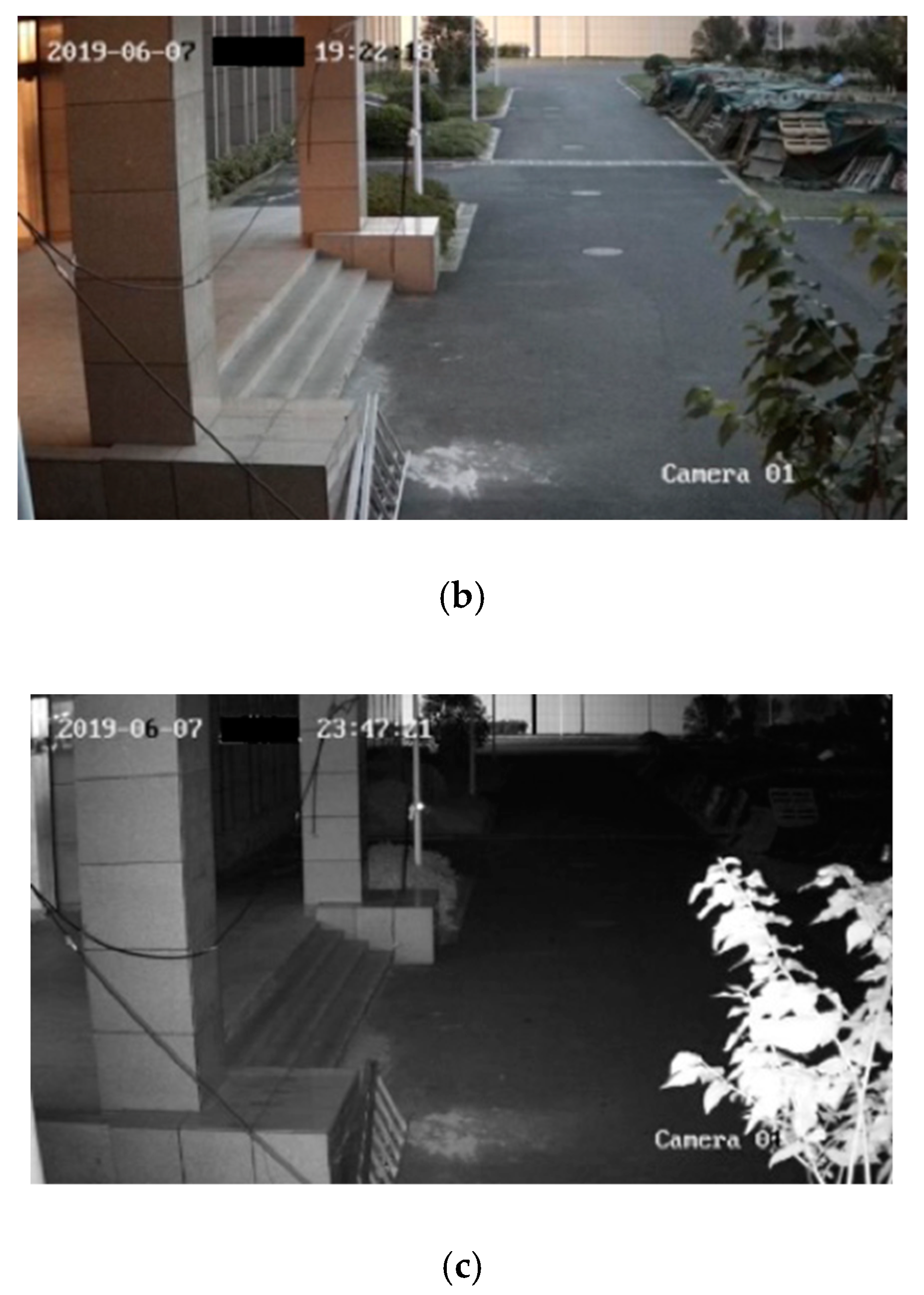
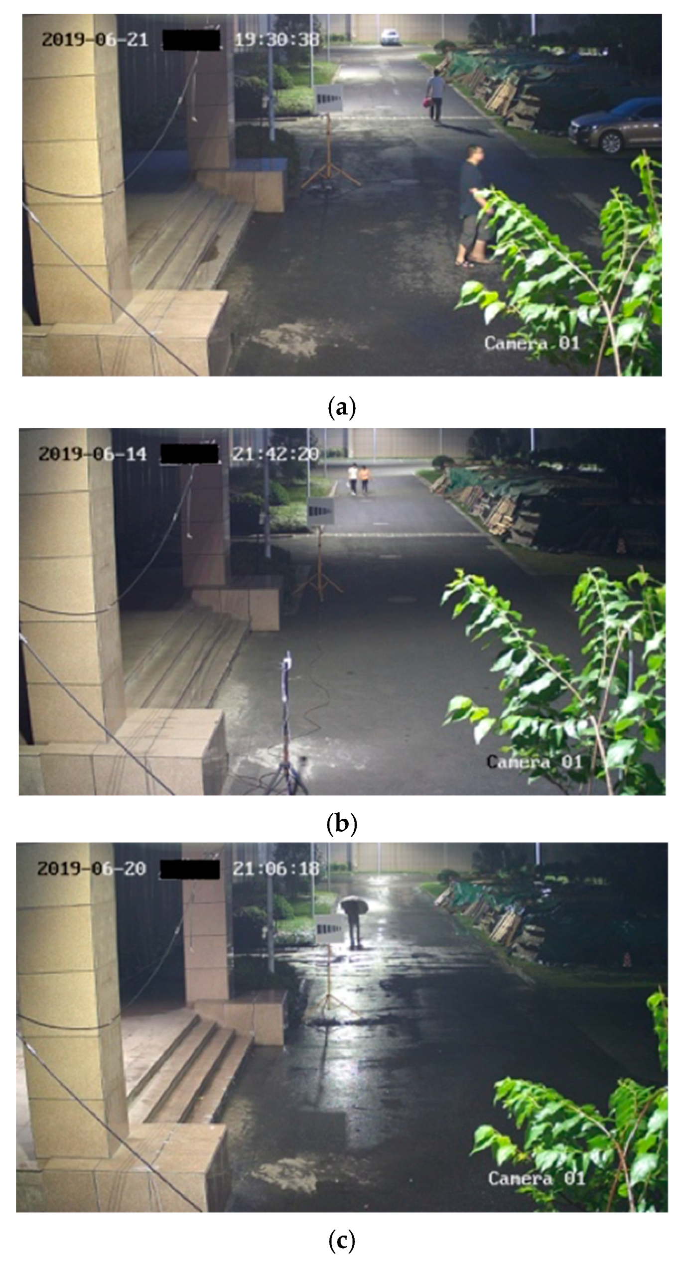
In different weather conditions such as sunny, foggy, and rainy days, pictures of the verification site were captured. Since both fog and rainfall can lead to low visibility, no distinction is made between fog and rainfall in practice. Approximately 600 verified images under different visibility conditions have been collected.
In some pictures, cars and pedestrians are set on the road at various distances to test the robustness of the method. Some samples of the original images are given in
Figure 7. The laser transmission scheme mentioned in
Section 3.1 is used to estimate the atmospheric transmissivity of the current state; the image analysis mentioned in
Section 3.2, to obtain the image characteristics; and the method mentioned in
Section 3.3, to assess visibility as a whole.
Table 3 shows the estimated visibility of the images in
Figure 7 and the errors between the estimated and measured values. The results show that the visibility estimation errors are within 20% when there are cars and pedestrians on the road, which has a certain degree of credibility.
In this paper, three values are presented for each image, which are based on the method used to derive the visibility, namely, laser transmission method alone (V1), image analysis method alone (V2), and proposed TSVE method (V). The estimated results and the errors with the visibility meter measurements of the six representative sample images in
Figure 8 are shown in
Table 4. It can be seen that the trend of the results obtained by using V1 is in line with the expectations. Both fog and rain can block out the transmission of the laser and lead to low visibility. The results obtained by using V2 are more inaccurate in the case of low visibility. Therefore, visibility must be calculated with the aid of laser transmission in the case of low visibility. Laser transmission and image analysis are required for reference in the case of high visibility. In addition,
Table 4 shows a significant difference in the visibility levels calculated by the three methods, where the V2 estimation error is higher than that of the V1. The estimation result of V1 is consistent with the trend of the visibility meter results, with the visibility level getting lower and lower from
Figure 8a to
Figure 8f. The estimated result of V does not match V1 result of
Figure 8d, and does not match V2 result of
Figure 8f, which to a certain extent agrees with the human perception of these images. In the case of visibility greater than 2000 m, the accuracy of our proposed TSVE method is less than 10%, and in the case of visibility below 2000 m, it is 10% to 30%.
We evaluate the proposed visibility algorithm by calculating the mean absolute error (MAE) [
2]. The MAE is defined as:
is the estimated visibility,
is the measured value by visibility meter,
,
N is the number of samples. The final experimental results in
Table 5 show that the proposed algorithm made fewer errors than V1 and V2. Some of the experimental images were captured in various common nighttime conditions (clear day, foggy, and rainy conditions), which shows that our algorithm has high accuracy under common nighttime weather conditions. In addition, experiments have shown that our approach provides better performance when data size increases.
Indeed, experimental verification of these methods is difficult. Taking photos in natural fog is a daunting task because weather conditions and fog uniformity cannot be controlled. Increasing the fog concentration of the environment through high-pressure spray equipment is also uneven. Our implementation is done through a target, which has some minor flaws. Using a purely “black” and larger target will result in a better estimate, but this is not realistic. In the future, we will test these methods with better cameras, measure the atmospheric extinction coefficient in a more precise way, and minimize or not use the target.
6. Conclusions
In this paper, we have presented a traffic perception visibility estimation algorithm that combines laser transmission and image processing. Nighttime road visibility was estimated by current atmospheric transmissivity and images characteristics, which include road image transmittance, target image transmittance, target brightness, and contrast. Multivariate nonlinear regression analyses were performed on various visibility indicators; two regression models with ambient brightness and without ambient brightness were established. Different classifications and multiple data improved the accuracy of the estimation. This algorithm was suitable for road visibility estimation under different weather conditions, without camera calibration. Finally, the adjustment suggestions for nighttime road visibility were also given. Experiments show that our proposed method can accurately estimate nighttime road visibility. When applied to highways, the estimated visibility can be used to adjust the speed limit of expressways, thereby reducing the occurrence of traffic accidents.


