Robust and Efficient Corner Detector Using Non-Corners Exclusion

Abstract

Corner detection is a traditional type of feature point detection method. Among methods used, with its good accuracy and the properties of invariance for rotation, noise and illumination, the Harris corner detector is widely used in the fields of vision tasks and image processing. Although it possesses a good performance in detection quality, its application is limited due to its low detection efficiency. The efficiency is crucial in many applications because it determines whether the detector is suitable for real-time tasks. In this paper, a robust and efficient corner detector (RECD) improved from Harris corner detector is proposed. First, we borrowed the principle of the feature from accelerated segment test (FAST) algorithm for corner pre-detection, in order to rule out non-corners and retain many strong corners as real corners. Those uncertain corners are looked at as candidate corners. Second, the gradients are calculated in the same way as the original Harris detector for those candidate corners. Third, to reduce additional computation amount, only the corner response function (CRF) of the candidate corners is calculated. Finally, we replace the highly complex non-maximum suppression (NMS) by an improved NMS to obtain the resulting corners. Experiments demonstrate that RECD is more competitive than some popular corner detectors in detection quality and speed. The accuracy and robustness of our method is slightly better than the original Harris detector, and the detection time is only approximately 8.2% of its original value.

1. Introduction

Feature point detection is used as the fundamental step of image analysis and computer vision. As an important element, corner detection is still widely used today in applications including object detection, motion tracking, simultaneous localization and mapping, object recognition and stereo matching [1,2,3]. A corner detector can be successfully used for these tasks if it has good consistency and accuracy [4]. For this reason, a large amount of pioneering work has been performed on corner detection in recent years. These techniques can be broadly classified into two categories: intensity-based corner detectors [5,6,7,8,9,10] and contour-based corner detectors [11,12,13,14]. Both types of corner detectors have their respective merits and demerits.

The contour-based corner detectors are mainly based on the curvature scale space (CSS). An edge detector is used in these detectors, for example the Canny edge detector [15], to obtain planar curves parameterized by arc-length. They are smoothed by a set of multi-scale Gaussian functions. Then the curvature is calculated on each point of the curves smoothed by the Gaussian functions. Finally, the candidate corners will be comprised of the absolute maximum curvature points from which weak and false corners will be excluded by thresholds. In order to improve localization, some CSS-based corner detectors additionally use a corner tracking step [13]. These detectors perform well in corner detection, but they suffer from two main problems. First, the curvature estimation technique is sensitive to the local variation and noise on contours because it uses second order derivatives of curve-point locations. Second, the large-scale Gaussian functions fail to detect true corners while small-scale ones detect a number of false corners. In other words, scale selection is a difficult task. In order to overcome the aforementioned problems, the multi-scale detector based on the chord-to-point distance accumulation (CPDA) technique is developed [14]. However, the complexity of the CPDA corner detector is high and it is difficult to improve from the algorithm architecture, so it cannot be applied to many computer vision systems. Other novel techniques are also proposed to improve performance, including angle difference of principal directions [16], Laplacian scale-space [17] and so on. However, all the methods in this category do not detect every corner region in an image. In particular, they fail to detect corner regions formed by a texture [18].

The intensity-based detectors indicate the presence of a corner by using the first-order or second-order derivatives of images and calculating the corner response function (CRF) of each pixel. Moravec computes the local sum of squared differences (SSD) between an image patch and its shifted version in four different directions [5]. The point with the largest SSD in a certain range is determined as a corner. But this technique is dramatically sensitive to noise and strong edges. Smith and Brady developed the smallest univalue segment assimilation nucleus (SUSAN) method for corner and edge detection [7]. This method is mainly based on a circular mask applied to the interest region. The pixels which have similar brightness to the nucleus construct the univalue segment assimilating nucleus (USAN) area. However, the accuracy of this algorithm is heavily dependent on the threshold. If the threshold is too big or too small, corner detection errors will result. Rosten and Drummond proposed the feature from accelerated segment test (FAST) algorithm based on the SUSAN corner detector [9,10]. As with SUSAN, FAST also uses a Bresenham circle of radius 3 pixels as test mask. The difference is that FAST just uses the 16 pixels in the circle to decide whether a point is actually a corner. The FAST algorithm requires very short computation time, but it is very sensitive to noise and needs to be combined with other algorithms to improve its robustness. By developing Moravec’s idea, Chris Harris and Mike Stephens proposed the famous Harris corner detection algorithm, which is one of the most important corner detectors based on intensity [6]. It computes the SSD in any direction. Simultaneously, it enhances the stability and robustness of the algorithm by introducing Gaussian smoothing factor. However, the computational efficiency of the technique is observably low. E. Mair et al. developed the FAST algorithm by constructing the optimal decision tree [19]. Leutenegger et al. further proposed the binary robust invariant scalable keypoints (BRISK) algorithm by constructing a scale-space with the FAST score [20]. Alcantarilla et al. proposed a fast multi-scale detector in non-linear scale spaces [21]. Xiong et al. introduced directionality to FAST in order to avoid repeatedly searching [22]. These FAST-based algorithms aim to speed up detection efficiency and retain good performance.

In this paper, a robust and efficient corner detector improved from the Harris corner detector, named the robust and efficient corner detector (RECD), is proposed. It is worth noting that the number of corners of an image is generally far fewer than 1% of the whole pixels. Thus, a key idea behind our method is to exclude a very large number of non-corners before detection. Because the non-maximum suppression (NMS) of the original Harris corner detector is complex, using an improved efficient NMS to reduce the complexity is another key idea. The original algorithm detects corners by three major steps. First, the image gradients are computed by the convolution of Gaussian first order partial derivatives in x and y directions with the image. Second, the CRF of each pixel is computed. Last, the maximum points are retained by NMS. In order to reduce the complexity, we analyze the three steps carefully and conduct many experiments. The experiment results show that the RECD possesses good robustness and efficiency. The RECD can be used for many visual processing domains because of its high speed and good performance.

The remainder of this paper is organized as follows. In Section 2, we discuss briefly the Harris corner detector and two criteria for performance evaluation of corner detectors. Section 3 introduces our detector, with a description of the algorithm and its implementation details. Section 4 illustrates the results of comparative experiments and gives an analysis of the results. Finally, we conclude our paper in Section 5.

2. Related Work

2.1. Harris Corner Detection Algorithm

The Harris corner detector is based on computing the corner response function of each pixel in an image [6]. If it is the local maximum and greater than a threshold value, the pixel is considered to be a corner. The corner response function is calculated by the autocorrelation matrix as follows:

$$M(p)={\displaystyle \sum _{(x,y)\in W}\{[\begin{array}{cc}I{}_x{}^2(p)& I{}_{xy}(p)\\ I{}_{xy}(p)& I{}_y{}^2(p)\end{array}]\otimes \omega (p)\}=[\begin{array}{cc}A& C\\ C& B\end{array}]}$$

(1)

where I_x(p) and I_y(p) are the respective horizontal and vertical image gradients at position p, obtained by the convolution of Gaussian first order partial derivatives in x and y directions with the image, respectively. The ω(p) is a Gaussian filtering function.

Harris and Stephens [6] suggested that direct eigenvalue decomposition can be avoided by calculating the response function as follows:

$$R=\det (M)-k\times {(trace(M))}^2$$

(2)

where det(M) and trace(M) are, respectively, the determinant and the trace of the autocorrelation matrix in the Equation (1). The coefficient k is an empirical value, usually lying in the interval [0.04, 0.06]. The image pixel is selected as a corner if R is the local maximum and greater than a given threshold value.

2.2. Performance Measurements

In order to evaluate the invariance of the proposed approach under the various transforms such as addition of noise and affine transformation, we introduce consistency of corner numbers (CCN) criterion for measuring the stability of corner detectors.

Mohanna and Mokhtarian presented the concept of the CCN criterion [4], which is defined as (3).

$$CCN=100\times {1.1}^{-|N_t}{{}^{-N_o}}^{|}$$

(3)

N_o is the number of corners in the original image and N_t is the number of corners in the transformed image. Since stable corner detectors do not change the corner numbers from original image to transformed images, in terms of consistency, the value of CCN for stable corner detectors should be close to 100% [23]. CCN is close to zero for corner detectors with many false corners.

This criterion does not determine the quality of the detected corners in any way, and the correctness of corner detections is obtained by the accuracy (ACU) measure [4]. The ACU is defined as follows:

$$ACU=100\times \frac{\frac{N_a}{N_o}+\frac{N_a}{N_g}}{2}$$

(4)

where N_o is the number of the detected corners in the original image, N_a is the total number of matched corners when comparing the first set of corners (found using a corner detector) to the second set (ground truth) using a neighborhood test, and N_g is the number of corners in the ground truth. When the majority of the detected corners are ground truths, the value of ACU will be close to 100%. Otherwise the value of ACU will be close to zero. Note that the ground truth corners are created by human judgment.

3. Proposed Methods

Generally, a corner can be defined as the pixel of large gray change in two different directions. The RECD is mainly based on the Harris corner detector. To speed up this algorithm and enhance the robustness, the principle of the FAST algorithm is used in corner pre-detection to rule out many non-corners and retain those strong corners as real corners as described in Section 3.1. Those uncertain corners are looked at as candidate corners to process further with Harris. Then, gradient calculation is analyzed as described in Section 3.2. On the basis of the first two steps, we just conduct the Gaussian filtering at the neighborhood of the candidate corners, the size of the window is 5 × 5. We then only calculate the CRF of the candidate corners. This step is described in Section 3.3. 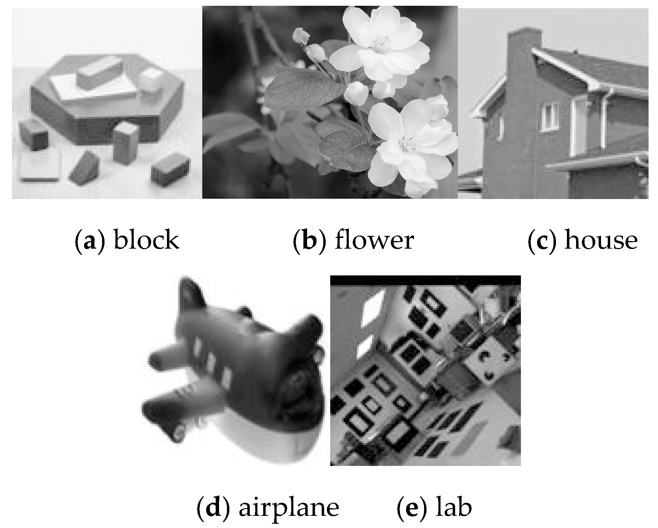Finally, the resulting corners are obtained by the improved NMS as described in Section 3.4. The test image sets we used are from standard databases [24,25] et al. In order to make the experimental results persuasive and convenient to compare with other methods, we selected these five images as test sets in the paper, which are shown in Figure 1.

3.1. Non-Corners Exclusion

The FAST theory has good robustness for transformations, especially for rotation, owing to the use of a circular template. A corner is generally at the vertex of a sharp angle on the image edge. Transformations change the structure of an angle to some extent. But the continuity of an edge is relatively robust. The FAST can detect out those structural corners and retain those uncertain corners from a transformed image. By contrast with the FAST, the Harris corner detector directly conducts gradient computation with a small window of 3 × 3 on the whole image. So the uncertain corners can be detected further with the Harris detector. If an uncertain corner is also validated by the Harris, it is a real corner.

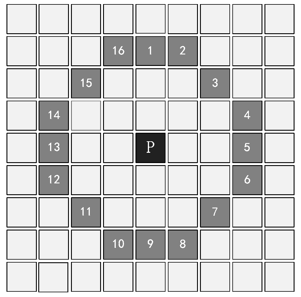
The key step of the FAST detector is that a circle of 16 pixels (a Bresenham circle of radius 3) is examined surrounding the point P as shown in the Figure 2. The point P is classified as a corner if the intensities of at least N contiguous pixels in the circle are all brighter (darker) than the intensity of the point plus (minus) a threshold t. N is actually a scale to judge the corners. Too large an N can lead to several missed corners and the small N will bring about too many weak corners. To ensure the accuracy and stability of the algorithm, N is generally set to 12.

In this paper, fast corner detection theory is applied to the first step: corner pre-detection. Three of the four pixels 1, 5, 9 and 13 certainly exist in these 12 contiguous pixels. We first examine the pixels 1 and 9. If both of the intensities of the two pixels are in a range of t of the intensity of the point P, then P is excluded to be a corner and the computation for current pixel is terminated. If not, we examine the pixels 5 and 13. If at least three of the four pixels are all brighter (darker) than the intensity of the point plus (minus) a threshold t, the point P is a corner. This is because 12 contiguous pixels are bound to include three of the pixels which will be examined. Note that if only two nearest neighborhood pixels in the four pixels, for example pixels 1 and 5, are both extremely brighter or darker than P, then P still can be a corner. We called these uncertain corners candidate corners. For an image of n × n pixels, the time complexity of this step is O(n²). Using this method can reject most non-corners, so that the computational complexity is reduced to a great extent for the next step gradient calculation. The FAST principle can only detect those obvious corners when there are 12 contiguous pixels in the circle of radius 3. For the situation of contiguous pixels less than 12, it does not perform well. This method can also detect some corners adjacent to one another. The pixels can be divided into three types by the FAST: non-corners, uncertain corners and strong corners. Therefore, we use this principle to exclude those non-corners and mark those strong corners as real corners. The uncertain pixels are all considered candidate corners to be detected further with Harris. In this case, almost all of the real corners are retained in the set of candidate corners and strong corners.

3.2. Gradient Calculation

Let the candidate corners be the center of a 3 × 3 neighborhood. After step A, we calculate the gradients in x and y direction of candidate corners after filtering the image with the level difference operator and the vertical difference operator, respectively. It is efficient to reduce computation complexity so that only the gradients of candidate corners are calculated without filtering the whole image in the Harris detector. After step A, a majority of background pixels of low-frequency parts are ruled out, because those pixels are easy to distinguish. We assume that m (m << n²) pixels remain as candidate corners. The computation complexity of the step B depends on the results of step A. Generally, the background contains a majority of pixels in an image and step A can filter out most of them and m is much less than n². It reduces many unnecessary operations in the background for the later steps. Actually, in the non-maximum suppression step, each pixel needs a 3 × 3 neighborhood to search the maximum of the CRF values. Thus, the gradients should be calculated for each pixel in this 3 × 3 neighborhood. Its time complexity is O (9m). In the Harris corner detector algorithm, this step has a time complexity of O (9n²).

3.3. Corner Response Function

The CRF step is computationally the most intensive and time-consuming stage of the Harris corner detector. The CRF of a pixel is calculated by determinant and trace of the autocorrelation matrix as in (2). The autocorrelation matrix is evaluated by Gaussian filtering for the squares and products of gradients as in (1). The CRF is calculated at each 3 × 3 neighborhood of candidate pixels. By employing the method in Section 3.1, we can reject a large number of non-corners. Then we only calculate the CRF based on the results of step B. Hence, this step can be accelerated drastically. Because many false corners are rejected in Section 3.1, the computational efficiency is improved much by calculating the CRF at the candidate corners. Also, the time complexity of this step depends on the m and it is O (9m).

3.4. Non-Maximum Suppression

NMS can be positively formulated as local maximum search [26]. In the original Harris corner detector, if the CRF of a pixel is the local maximum of its neighborhood and greater than a given threshold value, the pixel is considered to be a corner. The neighborhood is usually (2k + 1) × (2k + 1) region centered around the pixel under consideration. The NMS is performed at each pixel. However, there is one main problem with this approach. Once a local maximum is found, this would imply that we can skip all other pixels in the neighborhood of the maximum pixel point, because they must be smaller than the maximum point. For solving this problem, Neubeck and Gool proposed the efficient non-maximum suppression (E-NMS) method [26]. First, the algorithm partitions the input image into blocks of size (k + 1) × (k + 1). Then, it searches within each block for the greatest element. Finally, the full neighborhood of this greatest element is tested.Other pixels of each block can be skipped.

There is one main problem with the E-NMS algorithm. The areas of non-corners also execute the NMS procedure. This will inevitably increase complexity because of none existing corners. So, this paper improves the E-NMS algorithm. As an example shown in Figure 3, let the neighborhood window be equal to 3 × 3. By employing the method in Section 3.1, we have already calculated the candidate corners. First, we take a candidate corner as the center pixel to form a block of size 3 × 3 as shown in Figure 3a. Second, we search within the four candidate corners for the maximum element. Here, we assume that the p is the maximum element. The maximum of time complexity is O (9m) and the minimum is O (m). If the maximum of black blocks is not the center element P, the center pixel is abandoned and the next candidate corner is tested. Third, the full neighborhood is tested for the maximum element and the other three candidate corners in the block of size 3 × 3 will be skipped as shown in Figure 3b. Here the time complexity also can be taken as O (9m). Finally, we continue to test until traversing all candidate corners which do not include the skipped candidate corners. This step can effectively solve the main problem and play a role in accelerating the proposed method. For the Harris, this step takes O (9n²) owing to its operation for each pixel.

If the size of an image is very large with n, the total time complexity of Harris is O (9n² + n² + 9n²). The RECD takes O (n² + 9m + 9m + 10m) or O (n² + 9m + 9m + 18m). Thus if m < 4n²/7, the RECD has a faster speed. In fact, the m is far less than n² for a realistic image because many non-corners are excluded. The proposed RECD can improve the detection efficiency.

4. Experimental Results and Analysis

This section focuses on experiments and performance evaluation. The RECD is compared against a variety of other detectors such as Moravec [5], Harris [6], SUSAN [7] and FAST-9 [27,28] in terms of execution speed and the quality of the corner detection. The quality of the corner detectors is determined not only by the accuracy but also by the repeatability. We measured it based on the ACU and CCN criteria as described in Section 2. For the purpose of evaluation, a reference solution for each image is manually generated. Since there is no standard procedure to decide whether or not a point should be judged as a corner, only entirely obvious corners are included in the reference solutions [29].

4.1. Analysis of Accuracy

Accuracy requires that corners should be detected as close as possible to their correct positions [4]. The formula of ACU has been described in Section 2. We attempted the five test images, but due to lack of space only two test images are depicted in this paper. The ground truths of the block image and the lab image are illustrated in Figure 4, where the block image has 60 strong corners and the lab image has 242 strong corners. The corners for the two test images by the five algorithms are shown in Figure 5 and Figure 6. Each detector includes adjustable parameters and their settings affect detection results [30]. To give a fair evaluation, several tests have been conducted with each algorithm to attain individual optimal parameter settings.

We count the numbers of True Positives, False Negatives and False Positives for the five algorithms of the block and the lab. The results are listed in

Table 1. Evaluation results of the block image.

Detector	True Positives	False Negatives	False Positives	ACU
Moravec	39	21	16	0.680
SUSAN	28	32	36	0.452
FAST-9	47	13	9	0.811
Harris	48	12	1	0.890
RECD	48	12	1	0.890

and

Table 2. Evaluation results of the lab image.

Detector	True Positives	False Negatives	False Positives	ACU
Moravec	148	94	58	0.665
SUSAN	61	181	134	0.282
FAST-9	142	100	55	0.654
Harris	156	86	49	0.703
RECD	157	85	47	0.709

, where the True Positives refers to positive examples that are classified as positive examples. The False Negatives refers to positive examples that are classified as negative examples. The False Positives refers to negative examples that are classified as positive examples. The ACU means accuracy of the correctness of corner detections. It can be seen from Table 1 that the number of true corners is 60. The RECD and the Harris corner detector give the same results. Both detect the highest number of true positives and have the least number of false negatives and false positives. The FAST-9 corner detector performs slightly worse than the Harris corner detector and the RECD, but it performs substantially better than the Moravec detector and the SUSAN detector. The detection performance of the SUSAN corner detector is the worst. Similar results are shown in Table 2. However, the FAST-9 corner detector is now slightly worse than the Moravec corner detector in detecting true positives and false negatives, while the RECD performs slightly better than the Harris corner detector. It is noted that the RECD always performs best on accuracy. Subjective observation of the two experimental figures shows that the RECD detects the largest number of the true positives while it detects the least false negatives and false positives.

4.2. Consistency of Corner Numbers

Consistency means corner numbers should not vary with various transforms [4]. The formula of CCN has been described in Section 2. Here, the block image is used as test image to evaluate the consistency. According to the definition of CCN, its computation does not need the ground truths of test images. The number and the position of corners in the block image are shown in Figure 5. To evaluate the consistency of the five corner detectors, the rotation transformation, the shearing transformation, the brightness transformation, the uniform scaling and the Joint Photographic Experts Group (JPEG) compression are performed. The original image is first transformed with these transformations. Then, we use the five corner detectors to extract the number and the position of corners in all transformed images. Finally, the values for the CCN criterion are computed. The transformation factors are as follows:

• Rotation: 19 different angles in [−90°, 90°] at 10° apart.
• Shearing: the shearing factor of y direction in [−1, 1] at 0.2 apart.
• Uniform scaling: 11 scaling factors in [0.5, 1.5] at 0.1 apart.
• Brightness variation: 9 brightness factors in [0.2, 1.8] at 0.2 apart.
• JPEG compression: the quality loss factors in [0.1, 1] at 0.1 apart.

The Figure 7 shows the average consistency of corner numbers (CCN) under each transformation for five corner detectors. Figure 8 shows the CCN values of the five corner detectors under different shearing factors in vertical direction.

It can be seen that the proposed RECD achieves the best performance when shearing factor is in [−0.2, 0.4]. The Harris performs better than the RECD in the range from −1 to −0.4. Although the FAST-9 has better CCN at the shearing factor −0.6 and 0.6, it has large fluctuation and achieves low value at other shearing factors. As the basis of FAST−9, the SUSAN detector achieves similar results. The consistency of Moravec detector is the worst. It can be seen from Figure 7 that the average CCN value of RECD is highest which is followed slightly by Harris.

The consistency performance under uniform scaling is shown in Figure 9. It is obvious that RECD detector is the most stable one for the variation of scaling factor. Moreover, it performs best when the scaling factor is in [1, 1.3] and [0.6, 0.7]. As the basis of RECD, Harris has similar CCN to it. However, RECD has better consistency owing to the strong corner validation in Section 3.1. When the image is shrunk, FAST-9 achieves the best performance followed by RECD. By contrast, it performs worst when the image is enlarged. In Figure 7, the RECD has the best average CCN. It demonstrates that RECD has better detection capability under scaling transformation than the other four detectors.

Figure 10 shows the relation between CCN and image brightness. When the brightness factor is 1, the image is not changed. It becomes darker when brightness factor is less than 1 and brighter when brightness factor is more than 1. RECD and Harris both have a more stable curve and achieve better performance than other three detectors in Figure 10. FAST-9 performs worst under brightness variation. Seen from Figure 7, the RECD has highest average CCN under different brightness variations.

Figure 11 shows the consistency performance of the five detectors under different JPEG compression factors. The quality loss factor determines the percent of lost image information. As the increase of quality loss factor, the lost information increases. Obviously, the Moravec detector achieves the highest CCN. This is because the Moravec detector is more sensitive to edges of different directions. FAST-9 performs worst for JPEG compression seen from Figure 11. Figure 7. Shows the average CCN under each transformation for five corner detectors. It can be seen that the average CCN of the RECD detector is the second best under compression and slightly more than SUSAN and Harris.

For image rotation as shown in Figure 12, the average consistency of the RECD is highest at most of the rotation angles. Its invariance to rotation is better than the other four corner detectors. The Moravec corner detector shows the worst consistency, because the corner measures of the detector are highly sensitive to rotation. Although the average consistency of the RECD is highest, its consistency is obviously lower than the FAST-9 corner detector and SUSAN corner detector in the angle range of 20° to 30° and significantly higher than both of them in the angle range of 40° to 55°. No matter how much the angle of rotation is, the consistency of the Moravec corner detector is the worst. Through observation of Figure 12 and Figure 7, The RECD detector performs best under rotation transformation and is followed by the FAST-9 corner detector. The Harris detector performs better than the SUSAN corner detector and worse than the FAST-9 corner detector.

Compared with other four detectors, the proposed RECD detector achieves better consistency under shearing, scaling, brightness variation and rotation. It has the second best consistency under lossy JPEG compression. The RECD corner detector combines the merits of FAST and Harris. The non-corners exclusion step eliminates the interference of many non-corners and reduces the amount of computation of following steps. Thus, the following steps can detect fewer false corners without interference of those non-corners. As a result, the final corners obtained by RECD are more robust than the FAST-9 detector and Harris corner detector.

Image compression can retain the high-frequency information such as edges in an image. The Moravec detector chooses the edge direction with minimum variance to detect corners. It can extract many pixels on image edges although some are not corners. This is the reason why the Moravec detector performs best under JPEG compression.

4.3. Computational Time Performance

All the timing experiments are operated on Matlab R2014a with a 3.20 GHz Pentium(R) dual-core central processing unit (CPU) and 2 GB random access memory. To get more reasonable results, the five corner detectors are executed 100 times and mean execution times are measured. The time is obtained through the timing function in Matlab (tic/toc).

Table 3. Execution time of the five corner detectors.

Detector	Time (s)					Speed up (%)
	Block	Flower	House	Airplane	Lab
RECD	0.100	1.014	0.102	0.138	0.814	100.0
Moravec	0.561	6.166	0.559	0.977	2.251	20.6
SUSAN	1.010	12.002	1.111	1.856	4.391	10.6
Harris	1.239	16.155	1.307	2.280	5.266	8.2
FAST-9	0.293	2.427	0.340	0.449	1.326	44.8

and Figure 13 show the execution time of the RECD compared with other corner detectors. The speedup is relative to the performance of the RECD which represents the ratio of each referenced detector to the RECD. The computing method of the speedup is shown as (5):

$$speedup=\frac{t_1}{t_2}$$

(5)

where t₁ represents the execution time of the RECD and t₂ represents the execution time of one of the five corner detectors. The smaller the value of speedup, the more obvious the speed advantage of RECD over this compared method.

Figure 13 is Contrast of execution time of the five corner detectors. The RECD is the fastest among the five corner detectors while the conventional Harris corner detector is the slowest. The speed of RECD is more than 10 times faster than the traditional Harris angle detector.

As can be seen in Figure 13, compared with other detectors, the speed advantage is also obvious: the execution time of RECD is only 20.6% and 10.6% of Moravec and SUSAN respectively. Even with the closest FAST-9, our method has more than doubled the speed. This is enough to show that the speed improvement of RECD is significant. Note that the FAST-9 detector is different from the original FAST detector. It involves a machine-learning step to refine the result after the FAST step with 9 contiguous pixels. That is why the FAST-9 is slower than RECD.

5. Conclusions

In this paper, a robust and computationally efficient corner detector is proposed based on the Harris corner detector [6]. First, we used the theory of the feature from accelerated segment test (FAST) algorithm [9] to exclude a large number of non-corners and mark those strong corners. For those uncertain corners, they are judged as candidate corners and processed further. Second, we calculated the gradients in x and y directions of the image by filtering the candidate corners. Third, we calculated the corner response function (CRF) of the candidate corners. Finally, we used the improved efficient non-maximum suppression (NMS) to obtain the resulting corners. Consequently, we achieved a corner detector of good detection quality and high speed. The detection and localization performance evaluation were carried out using two theoretical criteria of the consistency of corner numbers (CCN) and accuracy (ACU). The experimental results show that the RECD is more accurate with respect to the ACU criterion and more robust with respect to the CCN criterion under all the five transformations except compression. Moreover, the RECD shows the fastest computation time among the five corner detectors. The detection time of the RECD is only approximately 8.2% that of the original Harris corner detector.

References

1. Pang, Y.; Cao, J.; Li, X. Learning sampling distributions for efficient object detection. IEEE Trans. Cybern. 2017, 47, 117–129. [Google Scholar] [CrossRef] [PubMed] [Green Version]
2. Yan, C.; Xie, H.; Chen, J.; Zha, Z.; Hao, X.; Zhan, Y. A fast Uyghur text detector for complex background images. IEEE Trans. Multimed. 2018, 20, 3389–3398. [Google Scholar] [CrossRef]
3. Zhang, S.; Liu, W. Single image 3D reconstruction based on control point grid. Multimed. Tools Appl. 2018, 77, 1–19. [Google Scholar] [CrossRef]
4. Mohanna, F.; Mokhtarian, F. Performance evaluation of corner detectors using consistency and accuracy measures. Comput. Vis. Image Underst. 2006, 102, 81–94. [Google Scholar]
5. Moravec, H. Towards automatic visual obstacle avoidance. In Proceedings of the 5th International Joint Conference on Artificial Intelligence, Cambridge, MA, USA, 22–25 August 1977. [Google Scholar]
6. Harris, C.; Stephens, M. A combined corner and edge detector. In Proceedings of the Alvey Vision Conference, Manchester, UK, 31 August–2 September 1988. [Google Scholar]
7. Smith, S.M.; Brady, J.M. SUSAN-A new approach to low-level image. Int. J. Comput. Vis. 1997, 23, 45–78. [Google Scholar] [CrossRef]
8. Trajkovic, M.; Hedley, M. Fast Corner Detection. Image Vis. Comput. 1998, 16, 75–87. [Google Scholar] [CrossRef]
9. Rosten, E.; Drummond, T. Fusing Points and Lines for High Performance Tracking. In Proceedings of the 10th IEEE International Conference on Computer Vision, Beijing, China, 17–21 October 2005. [Google Scholar]
10. Rosten, E.; Reitmayr, G.; Drummond, T. Real-Time Video Annotations for Augmented Reality. Adv. Vis. Comput. 2005, 3804, 294–302. [Google Scholar]
11. Rattarangsi, A.; Chin, R.T. Scale-based detection of corners of planar curves. IEEE Trans. Pattern Anal. Mach. Intell. 1992, 14, 430–449. [Google Scholar] [CrossRef]
12. Mokhtarian, F.; Suomela, R. Robust image corner detection through curvature scale space. IEEE Trans. Pattern Anal. Mach. Intell. 1998, 20, 1376–1381. [Google Scholar] [CrossRef] [Green Version]
13. He, X.C.; Yung, N.H.C. Corner detector based on global and local curvature properties. Opt. Eng. 2008, 47, 1–12. [Google Scholar]
14. Awrangjeb, M.; Lu, G. Robust image corner detection based on the chord-to-point distance accumulation technique. IEEE Trans. Multimed. 2008, 10, 1059–1072. [Google Scholar] [CrossRef] [Green Version]
15. Canny, J. A Computational Approach to Edge Detection. IEEE Trans. Pattern Anal. Mach. Intell. 1986, 8, 679–698. [Google Scholar] [CrossRef] [PubMed]
16. Zhang, W.C.; Shui, P.L. Contour-based corner detection via angle difference of principal directions of anisotropic Gaussian directional derivatives. Pattern Recognit. 2015, 48, 2785–2797. [Google Scholar] [CrossRef]
17. Zhang, X.; Qu, Y.; Yang, D.; Wang, H.; Kymer, J. Laplacian Scale Space Behavior of Planar Curve Corners. IEEE Trans. Pattern Anal. Mach. Intell. 2015, 37, 1. [Google Scholar] [CrossRef] [PubMed]
18. Mainali, P.; Yang, Q.; Lafruit, G.; van Gool, L.; Lauwereins, R. Robust Low Complexity Corner Detector. IEEE Trans. Circuits Syst. Video Technol. 2011, 21, 435–445. [Google Scholar] [CrossRef]
19. Mair, E.; Hager, G.D.; Burschka, D.; Suppa, M.; Hirzinger, G. Adaptive and generic corner detection based on the accelerated segment test. In Proceedings of the European Conference on Computer Vision, Crete, Greece, 6–9 September 2010. [Google Scholar]
20. Leutenegger, S.; Chli, M.; Siegwart, R.Y. BRISK: Binary robust invariant scalable keypoints. In Proceedings of the 2011 International Conference on Computer Vision, ICCV 2011, Barcelona, Spain, 1 March 2011. [Google Scholar]
21. Alcantarilla, P. Fast explicit diffusion for accelerated features in nonlinear scale spaces. IEEE Trans. Pattern Anal. Mach. Intell. 2013, 34, 1281–1298. [Google Scholar]
22. Xiong, W.; Tian, W.; Yang, Z.; Niu, X. Improved FAST corner-detection method. J. Eng. 2019, 2019, 5493–5497. [Google Scholar] [CrossRef]
23. Zhang, X.H.; Lei, M.; Yang, D.; Wang, Y.; Ma, L. Multi-scale curvature product for robust image corner detection in curvature scale space. Pattern Recognit. Lett. 2007, 28, 545–554. [Google Scholar] [CrossRef]
24. Petitcolas. Photo Database. Available online: http://www.petitcolas.net/fabien/watermarking/image_database/ (accessed on 2 January 2020).
25. The Usc-Sipi Image Database. Available online: http://sipi.usc.edu/database/ (accessed on 2 January 2020).
26. Neubeck, A.; van Gool, L. Efficient non-maximum suppression. In Proceedings of the International Conference on Pattern Recognition, Hong Kong, China, 20–24 August 2006. [Google Scholar]
27. Rosten, E.; Drummond, T. Machine Learning for High Speed Corner Detection. In Proceedings of the 9th European Conference on Computer Vision, Graz, Austria, 7–13 May 2006. [Google Scholar]
28. Rosten, E.; Porter, R.; Drummond, T. Faster and Better: A Machine Learning Approach to Corner Detection. IEEE Trans. Pattern Anal. Mach. Intell. 2010, 32, 105–119. [Google Scholar] [CrossRef] [PubMed] [Green Version]
29. He, X.C.; Yung, N.H.C. Curvature scale space corner detector with adaptive threshold and dynamic region of support. In Proceedings of the International Conference on Pattern Recognition, Cambridge, UK, 26 August 2004. [Google Scholar]
30. Shui, P.L.; Zhang, W.C. Corner Detection and Classification Using Anisotropic Directional Derivative Representations. IEEE Trans. Image Process. 2013, 22, 3204–3218. [Google Scholar] [CrossRef] [PubMed]
Figure 1. The images used for the performance test are block (256 × 256), flower (1024 × 576), house (256 × 256), airplane (331 × 361) and lab (512 × 512).
Applsci 10 00443 g001
Figure 2. Feature from accelerated segment test (FAST) corner detection in a Bresenham circle of radius 3.
Applsci 10 00443 g002
Figure 3. The improved efficient non-maximum suppression (E-NMS) algorithm. The black blocks are the candidate corners. The white blocks are the non-corners. The candidate corner p is the center pixel. (a) 3 × 3 block centered on candidate corner. (b) The neighborhood around that block.
Applsci 10 00443 g003
Figure 4. Test images (a) block and (b) lab and their ground truths where corners are labeled.
Applsci 10 00443 g004
Figure 5. Corner detection on the block image. (a) Moravec. (b) Smallest univalue segment assimilation nucleus (SUSAN). (c) FAST-9. (d) Harris. (e) Robust and efficient corner detector (RECD).
Applsci 10 00443 g005
Figure 6. Corner detection on the lab image. (a) Moravec. (b) SUSAN. (c) FAST-9. (d) Harris. (e) RECD.
Applsci 10 00443 g006
Figure 7. The average CCN under each transformation for five corner detectors.
Applsci 10 00443 g007
Figure 8. Consistency of corner numbers (CCN) of each method under shearing transformation.
Applsci 10 00443 g008
Figure 9. CCN of each method under uniform scaling transformation.
Applsci 10 00443 g009
Figure 10. CCN of each method under brightness variation.
Applsci 10 00443 g010
Figure 11. CCN of each method under JPEG compression.
Applsci 10 00443 g011
Figure 12. CCN of each method under rotation transformation.
Applsci 10 00443 g012
Figure 13. Contrast of execution time of the five corner detectors.
Applsci 10 00443 g013