1. Introduction
It is widely acknowledged that the number and diversity of water-related challenges are large and are expected to increase in the future. So, hydrological modeling can be efficient in order to analyze, understand, and explore solutions for sustainable water management in order to support decision-makers and operational water managers [
1]. In recent years, many water-experts have tried to use a range of methods for predicting hydrological components such as streamflow [
2]. The prediction of streamflow is essential in many aspects of water resources management, for example, reservoir operation and allocation. Also, streamflow can directly interfere with floods, droughts, agricultural issues, drinkable water supply, and all water-related systems [
3]. Predicting streamflow has been conducted by researches on different scales such as hourly scales [
4], daily scales [
5], 10 days scales [
6,
7,
8], monthly scales [
9], and annual scales [
10]. It is a difficult and challenging task for modelers to predict streamflow due to its complex (nonlinear) and non-deterministic characteristics. Hence, the execution of all simulation and predicting models is strongly based on the quality of the input data [
11]. Data-Driven models (DDMs), which are a combination of two main groups called Artificial Intelligence (AI) and time-series methods, are popular because of the ability to compute, their influential theory, and their implicit process in modeling [
12].
Recent reviews have shown that there is a great range of DDMs (such as ELM and CHAID) application for hydrological variables modeling, conducting several types of research in various topics such as daily water temperature [
13], daily streamflow [
5], dissolved oxygen concentration [
14], and salinity data [
15] estimation. Yadav et al. considered the Online Sequential ELM (OSELM) model for flood forecasting in the case of Neckar River, Germany. They tested the applied model by three evaluation techniques, and their results were compared with commonly used models like Support Vector Machines (SVM), Artificial Neural Networks (ANN), and genetic programming and they found out that the OSELM method can be used as a flood events alerting method rather than the aforementioned methods [
16]. Yaseen et al. conducted the OPELM model for the Tigris River in Iraq, and they used five groupings of inputs with lagged data. However, the results of the OPELM method were compared with the results of two other models, namely Support Vector Regression (SVR) and Generalized Regression Neural Network (GRNN) and it has been found that the OPELM model is superior in comparison to the previously mentioned methods [
17]. Rezaie-Balf and Kisi conducted three different soft computing methods, including Multilayer Perceptron Neural Network (MLPNN), OPELM, and evolutionary polynomial regression (EPR) as the sole model in forecasting daily streamflow in three stations on the Tajan River of Iran. The outcomes of this study reveal that the EPR method performed better than two other methods [
5].
CHAID model is one of the classification based techniques, which is used in determining the linearity or non-linearity of streamflow processes [
18,
19,
20,
21]. Althuwaynee et al. conducted CHAID and Multivariate Logistic Regression (MLR) models for extracting landslide maps in the case of the Pohang-Kyeong Joo catchment (Korea). The outcomes showed that both models have excellent efficiency in mapping [
22]. DDMs have some advantages and disadvantages in estimating the deterministic part of streamflow equations. For example, they are excellent for modeling the deterministic and algebraic parts of these variables, but they are not so useful for modeling the stochastic part of streamflow because of its nonlinear behavior. To overcome this issue, it would be worthwhile for experts to endeavor to use linear and non-linear time-series models (e.g., AR, ARMA, ARIMA, ARCH, Smooth Transition Autoregressive (STAR), Self-Exciting Threshold Autoregressive (SETAR), Bilinear models) to define the stochastic parts of models [
23,
24,
25,
26,
27], which are widely used in predicting hydrological variables like precipitation [
28,
29], streamflow [
30,
31], and runoff [
32,
33].
Several studies have carried out nonlinear, parametric and nonparametric methods like ARCH, STAR, SETAR [
20,
34] in predicting streamflow from reservoirs [
12,
35,
36,
37,
38], in modeling stage–discharge curves [
39,
40], and in the impact of climate change on runoff [
41]. The use of hybrid models in both AIs and time-series methods has been recently conducted by researchers worldwide [
42,
43,
44,
45,
46,
47]. The main goal of utilizing hybrid methods is to make prediction models concise by producing very remarkable and reliable results. Fathian et al. developed a nonlinear hybrid time-series, namely SETAR-GARCH, generalized autoregressive conditional heteroscedasticity, modeling streamflow in the case of Zarrineh Rood River at Urmia Lake Basin (ULB). They found that SETAR-GARCH models performed better than the models without GARCH, showing that the hybrid method performed better in modeling than sole models [
48]. However, the integration of AI and time-series methods with accuracy and optimum results is still scarce for hydrological phenomena such as streamflow. Mehdizadeh et al. proposed two new combined models of GEP-ARCH and ANN-ARCH methods in estimation of monthly rainfall in five selected stations of Iran. Their outcomes indicated that hybrid models outperform the sole models [
49].
The core objective of the present research is to develop a stronger and more accurate model for predicting monthly streamflow data using its antecedent values at two stations of Tapik and Dizaj in the Nazluchai and Baranduzchai rivers located in ULB of Iran, respectively for a period of 31 years. That is, this study aims to define new ARCH-type family models that can be used to obtain the stochastic terms of the streamflow equations. Although several studies have been carried out using linear and nonlinear time-series methods for hydrological forecasting, there is not any published work, to the best knowledge of the authors, related to the application of ARCH model integrated with two DDMs such as OPELM and CHAID (classification based technique) in predicting monthly streamflow. Another objective of this study is to assess the robustness of the hybrid OPELM/CHAID-ARCH vs. standalone models viz diagnostic evaluation of performance with visual plots and statistical score metrics of predicted and observed streamflow for the independent validation data.
The rest of the present research is organized as follows.
Section 2, which is considered as the materials and methods, includes
Section 2.1, study area and data analysis;
Section 2.2,
Section 2.3,
Section 2.4,
Section 2.5 and
Section 2.6, describing the methodology of nonlinear models (ARCH) and two DDMs (e.g., CHAID and OPELM) and their integration; and
Section 2.7, describing the statistical performance indicators applied for this study.
Section 3.1,
Section 3.2,
Section 3.3,
Section 3.4,
Section 3.5 and
Section 3.6 discusses the forecasting results of the proposed models and comparative results.
Section 3.7 is the discussion and, finally,
Section 4 presents a summary, future work, and the conclusion of the outline results are given.
2. Material and Methods
2.1. Study Area and Data Analysis
Two rivers, named Baranduzchai and Nazluchai for full streamflow data, and with two measurement stations, named Dizaj and Tapik, in the ULB in Iran, were considered. The Baranduzchai River has an area of 1203 km
2 and is located in the north-west of Iran between Urmia Lake, Iraq, and Turkey, at 44°45′ to 45°14′ latitude and 37°06′ to 37°29′ longitude. The stream is 75 km long, and the basin’s maximum altitude is 1250 m. It has four hydrometric stations named Babarud, Dizaj, Gasemlu, and Bibakran. The Nazluchai River is almost 93 km long and has an area of 2030 km
2. Almost 90% of this stream is located in Iran, with the remaining 10% in Turkey. The stream’s maximum altitude is 3600 m. It has four hydrometric stations named Abajalu, Tapik, Karim Abad, and Marz Sero. In this research, Dizaj and Tapik stations were selected, as shown in
Figure 1.
In the present study, the dataset contained 31 years of monthly streamflow data (372 months) from January 1986 to December 2016. These data were obtained from the Urmia Lake Research Institute (ULRI) in Urmia, Iran. In this study, 70% and 30% of data from the beginning (260 months and 112 months) were used for calibration and validation stages, respectively.
Figure 2 shows the monthly streamflow data in both stages for this period.
The geographical and statistical properties of monthly discharge of both streams are shown in
Table 1 and
Table 2, respectively. As can be seen from
Table 2, standard deviation values are higher than skewness values in both river gauges. It is worth mentioning that these statistical properties have been calculated before normalization of data, and they belong to the only streamflow data before any changes.
2.2. ARCH-Type Models
By applying nonlinear models to hydrologic processes, especially streamflow modeling, it is worth mentioning that the conventional linear models primarily focus on the average of data (first-order moment) because they do not consider the second moment of data (variance), thus, their application is not enough for modeling stochastic data. By using linear models, experts cannot seize the nonlinear characteristics of hydrological data [
48]. Besides, methods for working with changes to variance over time are necessary for water resources management developments [
50]. Defining nonlinear methods for modeling variance variation is essential in modeling and forecasting. For this purpose, Engle (1982) introduced the ARCH model. Equations (1) and (2) illustrate the ARCH model [
51].
where
is conditional variance,
is a discrete-time stochastic process, and
is the ARCH model’s parameters,
q is the model’s order, and
zt is the normal and standard series.
This study presents 12 steps for modeling the stochastic parts of time-series using ARCH-type methods:
Step 1: Data collection. All stream data were first collected on a monthly scale.
Step 2: Data Preprocessing. It included checking data lengths, investigating statistical parameters, and data stationery.
Step 3: Data normalization. This used the Delleur and Karamouz method [
52] and defined the average and standard deviation of streamflow data.
Step 5: Fitting the best AR models to stream time-series data.
Step 6: Defining .
Step 7: Comparison of different ARCH-type models. At this point, the best-performing method was selected.
Step 8: Defining different scenarios for estimating the deterministic part of the modeling equations.
Step 9: Dividing data into two sections (calibration and validation). At this point, the best input combination and selection method can be defined.
Step 10: Running DDMs for defining the deterministic part of the streamflow modeling formula.
Steps 11 and 12: Selecting the best-performing hybrid model for estimating streamflow.
As a conclusion, autoregressive conditional heteroscedastic residuals occur when the ARCH model considers the assumption that all data are normal, but the conditional variance of the residuals fluctuates linearly with squared residuals. The main difference of ARCH models with the other time-series models like AR, MA, and ARMA is that they can be applied on squared residuals of data.
2.3. CHAID Model
CHAID was first developed by [
53]. CHAID algorithms, as well as CART models, are used for classification, and the outcomes are usually classification trees, which are nonparametric methods. In other words, these methods are called decision tree methods, while this tree offers specific rules along with their inputs and outputs. Each input variable in these methods is divided into subgroups. Despite black-box methods, the internal procedures of these tree models are visible for the user, and they have been called white-box methods [
54]. The main difference between decision trees and regression models is in their relations between their variables, in which there are simple linear combinations for regression methods with classification and categorization based on output variables in decision methods [
55].
CHAID algorithm uses Pearson’s Chi-square when a target variable is categorical and uses the likelihood ratio Chi-square statistic as a separation reference when a target variable is continuous. The function of likelihood ratio Pearson’s Chi-square statistic is calculated as [
53]
Overall, the steps of CHAID model application are as follows:
(1) The best division for each input variable is found.
(2) The best input variable was selected.
(3) The whole data were divided into subgroups.
(4) Each of these subgroups is divided into new subdivisions.
More detailed of this method can be found in [
55].
2.4. OPELM Model
OPELM is developed in order to select the weights of the hidden neurons of traditional ANN models, such as FFNN, which are known as AI techniques. OPELM was first introduced by [
56]. This algorithm has some advantages in comparison to a single-layer feedforward neural network (SLFN) and typical methods. SLFN contains an input layer, a hidden layer, and output layer [
57]. A typical SLFN with M samples, L hidden nodes, and h(x) as an activation function can be described as
By using the least-square method, OPELM picks input weights
w and biases
b and then calculates the output weights
β. In another way, activation function can be illustrated as below:
In which
H is the hidden layer output matrix and can be defined as
The main aim of OPELM [
58] is to minimize
that is equivalent to maximization of
. As discussed in [
59], utilizing OPELM algorithms can diminish the time for training models, and
i and
t also have simpler algorithms. In the OPELM algorithm, parameters of hidden nodes are selected randomly, and the output weights are calculated using the least-squares method [
60].
However, the OPELM algorithm has some problems with correlated data. Therefore, OPELM is based on the original algorithm of OPELM with some different and extra steps to make it vigorous by the pruning of the neurons. This algorithm was first introduced by [
59]. It relays on both classification and regression problems. The OPELM utilizes a leave-one-out (LOO) criterion for the selection of a suitable number of neurons [
5]. It also uses four types of kernel functions, namely Gaussian, sigmoid, linear and nonlinear. More information can be found in [
59].
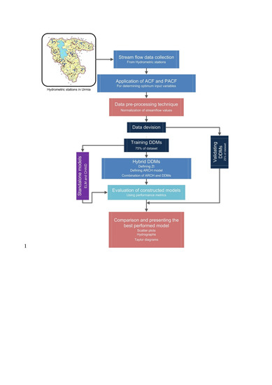
2.5. Hybrid Models Development
As previously highlighted, OPELM and CHAID models are defined as deterministic methods in which the equation of models is determined by initial parameters and values. On the other hand, stochastic models like ARCH have some intrinsic randomness in which using the same initial parameters and values will initiate a group of different outputs. After defining both the deterministic and random parts of the streamflow data using OPELM, CHAID, and ARCH models, new series were generated by combining these two parts. The combined ARCH-OPELM and ARCH-CHAID hybrid based model can be defined as
where
is the modeled deterministic part of the streamflow time-series by two methods of CHAID and OPELM and
is the modeled random part of the streamflow series. As shown in Equation (9), this formula was found to estimate both the deterministic and random parts of hydrological nonlinear events. In this study, the equation obtained from two methods of CHAID and OPELM models and the results of ARCH modeling are considered as
and
respectively. In other words, using the two-step process, the new integrated hybrid nonlinear model is established. In the first step, a linear deterministic model from OPELM and CHAID method is estimated in order to generate new values of monthly streamflow. In the second step, the ARCH model, which is nonlinear and estimated using the volatility forecasts, is plugged into the proposed models of OPELM and CHAID. As a result, new-formed models, namely ARCH-CHAID and ARCH-OPELM, are established. The process of the proposed hybrid (OPELM/CHAID-ARCH) models to predict monthly streamflow is shown in
Figure 3.
2.6. Optimum Antecedent Streamflow as the Input Variables
Input variables selection is one of the critical steps in every model creation. However, it might result in accurate and natural streamflow predictions. Since the streamflow is one of the physical and natural phenomena in the hydrological cycle, the modeler could be interfaced with a lot of candidate inputs, so defining optimum inputs could be helpful. In this research, the authors proposed optimum inputs by utilizing the Autocorrelation Function (ACF) and Partial Autocorrelation Function (PACF). The number of lags in order to model the AR model is defined by the number of non-zero lags in ACF. PACF can identify the correlation between the current month and the previous months. The number of lags that existed between the 95% confidence level in PACF was considered as the number of lags in monthly streamflow forecasting.
2.7. Performance Metrics
The outcomes of streamflow modeling with CHAID, OPELM, and hybrid ARCH-CHAID and ARCH-OPELM models were evaluated by five statistical metrics. The performance metrics utilized in this study were Correlation Coefficient (R), Root Mean Square Error (RMSE), Nash–Sutcliffe model efficiency coefficient (NSE), Mean Absolute Error (MAE), and the ratio of RMSE to the standard deviation (RSD).
(a) R: The closer is the value to 1, the higher the accuracy.
(b) RMSE: The smaller the RMSE, the more precise the prediction will be [
61].
(c) NSE: The closer the value is to 1, the higher the accuracy. The NSE is utilized to evaluate the predictive power of models [
62].
(d) MAE: The smaller the MAE, the more precise the prediction will be.
(e) RSD: The smaller the RSD, the more precise the prediction will be [
63].
Equations (10)–(14) give evaluations for assessing the accuracy of the models. In these equations, M is the number of observations, Oi is the actual observations, and Pi is the estimated values. Also, and denote the mean of the observed and predicted dataset, respectively, and STDEV represents standard deviation, in the studied period.
3. Application Results
As mentioned before, the streamflow dataset of two stations, namely Dizaj and Tapik, in north-western Iran, contained 31 years of data (372 months) from January 1986 to December 2016. In order to establish models, 70% and 30% of data from the beginning (260 months and 112 months) were used for calibration and validation stages of the proposed models. First, the quality of modeling starts with data pre-processing (data normalization). In the second step, two standalone models including OPELM and CHAID models were used to predict monthly streamflow. To improve predictive models, the stochastic term of streamflow models was calculated by ARCH model that described the variance of the current error term or innovation as a function of the actual sizes of the previous time periods’ error terms, and afterward, the results of hybrid (ARCH-OPELM and ARCH-CHAID) models were reported.
3.1. The Results of the Autocorrelation Function (ACF) and Partial Autocorrelation Function (PACF)
The correlograms of monthly streamflow, as an input variable determined by autocorrelation, and partial autocorrelation functions for both stations of Dizaj and Tapik were illustrated for 20 months. These figures demonstrate the true value of inputs for each station. With 95% confidence, the limits of ACF and PACF are given by ± 1.96/√
n, and were demonstrated by red color dash lines (
Figure 4). The lag number could be defined when the lags were considered between these two lines [
64]. As shown in
Figure 4, six months of lag were considered for Dizaj station as input variables; however, for Tapik station, lag number 4 was considered as the optimum input variable.
3.2. Data Preprocessing
In order to establish a platform for conducting the DDMs for streamflow modeling, this section provides some preliminary steps of data normalization as one of the preprocessing methods. The goal of normalization is to change the values of numeric columns in the dataset to use a standard scale, without distorting differences in the ranges of values. There are two primary advantages of data normalization, increased consistency (reducing the possibility) and easier object-to-data mapping (normalized data schemas are closer conceptually to object-oriented schemas), according to which data needs to be normalized for DDMs.
In the present research, firstly, streamflow data of Dizaj and Tapik stations were normalized by using Equation (3), and data standardization was calculated by Equation (4).
Table 3 shows the skewness of the data before and after the normalization. Before normalization, the skewness of the Baranduzchai and Nazluchai stations was 2.055 and 2.822, respectively. Using Equation (3), parameter C was extracted by trial and error; thus, the mentioned parameters were 0.714 and 0.268 for Baranduzchai and Nazluchai, respectively. Then, after the normalization process, skewness was obtained as −0.000187245 and 0.000861473 for Baranduzchai and Nazluchai, respectively.
3.3. Application Results of Standalone Models
In this study, a standalone well-designed OPELM algorithm and CHAID models were utilized by conducting the MATLAB and Statistica software, respectively. As demonstrated in
Figure 5, in order to assess the performance of standalone models, the results of streamflow by using both OPELM and CHAID models are compared with their historical and observed data for both Dizaj (the blue one) and Tapik (the red one) stations. In Dizaj and Tapik stations, the CHAID model showed better prediction performance by relying on the determination of the coefficient metric at the validation stage, while, in the comparison between two stations, the OPELM model performed better at Dizaj station. Overall, in the evaluation of these two standalone models for monthly streamflow prediction, it is interesting to conclude that the CHAID model as a DDM model appeared to be a better model in both candidate stations.
Table 4 brings the comparison standalone OPELM and CHAID models, which are developed for streamflow prediction at two selected stations (Dizaj and Tapik) in terms of five different indices, namely R, RMSE, NSE, MAE, and RSD. According to this table, in the calibration stage, Dizaj-OPELM had the highest R (R = 0.92). It was followed by Dizaj-CHAID and Tapik-OPELM (R = 0.91) and Tapik-CHAID (R = 0.90). In the case of root mean square errors, Dizaj-OPELM had the lowest error (RMSE = 3.378 m
3/s), and Tapik-CHAID had the highest error (RMSE = 7.816 m
3/s) while Tapik-OPELM (RMSE = 7.428 m
3/s) and Dizaj-CHAID (RMSE = 3.655 m
3/s) were located between these two values. As NSE, Dizaj-OPELM had the highest value (NSE = 0.84). It was followed by Dizaj-CHAID (NSE = 0.82), Tapik-OPELM (NSE = 0.81) and Tapik-CHAID (NSE = 0.79). By considering MAE, Dizaj-OPELM had the lowest error (MAE = 1.854 m
3/s). It was followed by Dizaj-CHAID (MAE = 2.144 m
3/s), Tapik-OPELM (MAE = 3.374 m
3/s), and Tapik-CHAID (MAE = 3.697 m
3/s). In the case of the ratio of RMSE to the standard deviation, Tapik-CHAID had the highest RSD value (RSD = 0.451). It was followed by Tapik-OPELM (RSD = 0.429), Dizaj-CHAID (RSD = 0.419), and Dizaj-OPELM (RSD = 0.387). The higher R and NSE values present a better-predicted model. In the comparison of two other parameters of RMSE and MAE, this table reveals that the calculated MAE values are about half of the RMSE values; the reason is that the RMSE evaluation metric gives special importance to large errors. For the validation stage dataset, CHAID had an R = 0.94, RMSE = 1.571 (m
3/s), NSE = 0.91, MAE = 1.863 (m
3/s) and RSD = 0.328 was considered as better model in Dizaj station and CHAID with an R = 0.89, RMSE = 4.329 (m
3/s), NSE = 0.77, MAE = 2.253 (m
3/s) and RSD = 0.473 was considered as the selected model in Tapik station.
3.4. ARCH Model
The ARCH-type models are nonlinear models that provide a platform for emphasizing the second-order momentum (variance) and the stochastic element of hydrological variables (in this research of streamflow). As part of ARCH development, the distribution used in this study was Gaussian white noise that the equation predicts the next month’s streamflow in principle of this month’s streamflow. With the purpose of estimating ARCH parameters, the log-likelihood method was used. The ARCH model is implemented by JMulti software. Using observed data and their variance, ARCH time-series for Dizaj and Tapik stations were calculated using a Gaussian method.
Table 5 shows the calculated models with their loglikelihood value. Since the Akaike Information Criterion (AIC) was unutilized for defining the lengths of lags.
3.5. Results for the Integration of OPELM, CHAID and ARCH Models
The ARCH model is combined with the best-resulted models OPELM and CHAID. The results of this part can be divided into two categories of ARCH-OPELM and ARCH-CHAID combinations.
Figure 6 looks at two combined models of ARCH-OPELM and ARCH-CHAID at both stations of Dizaj and Tapik. Focusing on calibration and validation stages in both stations,
Figure 6 shows excellent similarities between observed and modeled data in both calibration and validation stages at two stations of (a) Dizaj, (b) Tapik. In general, it reveals that ARCH-CHAID has more significant results of the determination coefficient in comparison to ARCH-OPELM combined models. In the right above, this figure represents scatterplots of both ARCH-OPELM and ARCH-CHAID models with their regression lines and correlation of determination (R
2). The regression equation, which is based on modeled and observed values of streamflow is obtained from
y (Gm) = aG
o + b. In which G
o stands for observed streamflow datasets, and
Gm stands for the modeled streamflow datasets. Based on a, b, and R
2 values, the best models could be selected. The results were a = 1.123, b = 2.8305, and R
2 = 0.8166 (for ARCH-OPELM), also a = 0.9616, b = 1.9938, and R
2 = 0.9201 (for ARCH-CHAID); in Dizaj station, the ARCH-CHAID model was selected as a better model. Also in Tapik station, the outcomes were a = 1.1633, b = 3.6354, and R
2 = 0.797 (for ARCH-OPELM), also a = 0.9163, b = 3.5381 and R
2 = 0.885 (for ARCH-CHAID) were obtained. The ARCH-CHAID model was selected in Tapik station based on the above-mentioned results.
In another way of comparing the performances of the hybrid models,
Table 6 summarizes the performance evaluation metrics outcomes of hybrid ARCH-OPELM and ARCH-CHAID models for Dizaj and Tapik stations. In the calibration stage, Dizaj-ARCH-OPELM had the highest R-value of 0.94. It was followed by Tapik-ARCH-CHAID (R = 0.93), Dizaj-ARCH-CHAID and Tapik-ARCH-OPELM (R = 0.92). Dizaj-ARCH-OPELM had the lowest error (RMSE = 2.168 m
3/s). It was followed by Dizaj-ARCH-CHAID (RMSE = 2.395 m
3/s), Tapik-ARCH-CHAID (RMSE = 5.678 m
3/s) and Tapik-ARCH-OPELM (RMSE = 6.896 m
3/s). In the case of the NSE coefficient, Tapik-ARCH-CHAID had the highest value (NSE = 0.85). It was followed by Dizaj-ARCH-CHAID (NSE = 0.83), Tapik-ARCH-CHAID (NSE = 0.82) and Tapik-ARCH-OPELM (NSE = 0.82). Similar to the RMSE metric, MAE metric had the highest value in Dizaj-ARCH-OPELM (MAE = 1.268 m
3/s). It is followed by Dizaj-ARCH-CHAID (MAE = 2.039 m
3/s), Tapik-ARCH-OPELM (MAE = 3.215 m
3/s), and Tapik-ARCH-CHAID (MAE = 3.167 m
3/s). In the case of the ratio of RMSE to the standard deviation, Tapik-ARCH-OPELM had the highest value (RSD = 0.422). It was followed by Tapik-ARCH-CHAID (RSD = 0.418), Dizaj-ARCH-CHAID (RSD = 0.348), and Dizaj-ARCH-OPELM (RSD = 0.319).
In the validation stage, Dizaj-ARCH-CHAID had the highest R-value of 0.96. It is followed by Tapik-ARCH-CHAID (R = 0.94), Dizaj-ARCH-OPELM (R = 0.91), and Tapik-ARCH-OPELM (R = 0.89). Dizaj-ARCH-CHAID had the lowest error (RMSE = 1.289 m3/s). It was followed by Dizaj-ARCH-OPELM (RMSE = 1.496 m3/s), Tapik-ARCH-CHAID (RMSE = 2.662 m3/s) and Tapik-ARCH-OPELM (RMSE = 3.671 m3/s). By considering NSE, Dizaj-ARCH-CHAID had the highest value (NSE = 0.92). It was followed by Tapik-ARCH-CHAID (NSE = 0.86), Tapik-ARCH-OPELM (NSE = 0.78), and Dizaj-ARCH-OPELM (NSE = 0.38). By considering MAE, ARCH-CHAID had the lowest value for both Dizaj and Tapik, respectively, 0.719 (m3/s) and 1.467 (m3/s) compared to other standalone and hybrid models. In the case of the ratio of RMSE to the standard deviation for Tapik station, ARCH-CHAID with RSD = 0.419 was better validated than the ARCH-CHAID (RSD = 0.487).
3.6. Comparison of Standalone and Hybrid Models
In order to compare standalone and hybrid models in streamflow prediction,
Figure 7 was used. The first graph shows the Taylor diagram of Dizaj station, while the second demonstrates the Tapik station diagram. These two diagrams represent the optimal predictions of four standalone and hybrid models of monthly streamflow prediction, namely OPELM, ARCH-OPELM, CHAID, and ARCH-CHAID models. These diagrams could represent graphically that which of the models has the closest prediction of streamflow with the historical calibration monthly streamflow data. All models compared graphically with three important evaluation metrics, namely correlation coefficient, standard deviation, and root mean square error (RMSD). Centered RMSD showed the reference point (observed value), and the distance of a particular model with this point shows the ideal model. As shown in the diagrams, the ARCH-CHAID model outperformed all other standalone and combined methods of DDM at two candidate study stations.
3.7. Discussion
On the one hand, as expressed earlier, streamflow and other hydrological variables have a nonlinear behavior, so that in modeling experts should consider both deterministic (algebraic) and stochastic parts of this parameter in order to make a proper decision for water resources management purposes [
48]. According to the above study results, the stochastic part of streamflow has extremely improved the performance of the sole-models, i.e., OPELM and CHAID, in terms of prediction. ARCH was introduced as a nonlinear parametric time-series approach that describes the behavior of the conditional variance of the data. In this regard, integration of ARCH with the fast and efficient ELM and CHAID models led to the newly developed ARCH-OPELM/CHAID models, which effectively ‘learns’ those two parts in emulating monthly streamflow.
On the other hand, one of the challenging issues is that the models can predict river flow accurately by chance or perform well only in some ranges of input and output variables [
65]. To respond to this circumstance, the current research considers two rivers in ULB with different characteristics of input and output variables in order to assess the applicability of the predictive models. It should be highlighted that this study tried to give some applications and models to ease the monthly time-scale forecasting of streamflow since the available data are very poor in quality and hard to achieve, especially in developing countries like Iran.
By the previous results, the better-predicting capability of ARCH-OPELM/CHAID in the monthly-time forecasting horizon is clear from the predictor metrics and the diagnostic plots at both the study sites. To evaluate the improvement achieved by the proposed models on the other two compared models of OPELM and CHAID, the performance promotion is fully exhibited in
Table 4, where the five performance metrics values are revealed. Remarkable performance improvement can be observed for all indices. The average promotion ratio of indices RMSE, MAE, and RSD of both two horizons are evident in confirming the improvements, in which the ARCH-ELM models for Dizaj and Tapik could decrease prediction error by 17% and 38%, respectively. This percentage for ARCH-ELM reaches about 41% (Dizaj) and 29% (Tapik) for validation stage.
According to the scatter plots, standalone OPELM and CHAID models show an under-predicted performance in the calibration stage for both Dizaj and Tapik stations, although this drawback improved by considering the stochastic process of streamflow integrating with ARCH time-series model. In the validation stage, the ARCH-OPELM based on histogram could predict river flow values as well as the ARCH-CHAID model. Thus the classification CHAID modeling method used in the study is confirmed as being a very useful tool to investigate the methods for forecasting streamflow on a monthly scale. The hybrid models were found to improve the streamflow prediction across the evaluation criteria for two stations of Dizaj and Tapik on two main streamflow of Nazluchai and Baranduzchai in ULB. The whole study revealed that the hybrid ARCH-DDMs could increase the performance of sole DDMs up to 10%.
As the perspective for real applications, it should be noted that providing a reliable model to forecast river flow could be instrumental for water resources planning and management [
5]. Hydrological forecasting plays an essential role in the investigation of physical mechanisms and the causes underlying changes therein. The results of forecasting can also be used for agricultural irrigation management, water resources management, flood warning, and the design and management of hydraulic structures [
66]. It is therefore not surprising that much attention has been devoted to the techniques of hydrological forecasting, development, and improvement of hydrological models, as well as the use of hydrological models in practice [
67,
68,
69,
70].
The challenges and barriers for high-accuracy forecasting of flow’s quantity are the nonlinearity and uncertainty hidden in the streamflow. An approach with high forecasting precision and efficiency would be qualified in the real application.
4. Conclusions and Future Work
Accurate forecasting of streamflow is a fundamental issue of interest to water resources engineers, scientists, and hydrologists. This research work implements and evaluates the efficiency of standalone (OPELM and CHAID) models for two different rivers, including Baranduzchai and Nazluchai in ULB, Iran. To access the optimum input variables, the PACF, which considered identifying the statistically significant lagged data to construct the models, was applied to select the relevant input variables of the final model for predicting streamflow. The inputs and the output quantities of the models were split into two subsets including calibration (70% of total dataset) and validation (30% of total dataset) phases, and then whole dataset was normalized as the pre-processing data phase in order to change the values of numeric columns in the dataset to a common scale. The performance of the developed models was evaluated in terms of R, RMSE, NSE, MAE, and RSD.
Afterward, to improve model performance for prediction of streamflow, the stochastic term of streamflow models was calculated by the ARCH model that describes the variance of the current error term or innovation as a function of the actual sizes of the previous time periods’ error terms. Therefore, the suitability of two hybrid models, ARCH-OPELM and ARCH-CHAID, has been examined and compared against standalone models (OPELM and CHAID) for streamflow modeling at two candidate study stations in ULB. The results remarkably reveal that ARCH-CHAID models in both stations outperformed all other models. Besides, standalone CHAID models have better results than OPELM methods. While ARCH-OPELM and OPELM models have ranked third and fourth in predicting monthly streamflow. As a conclusion, it is worth mentioning that the new hybrid “ARCH-DDM” models outperformed standalone models in predicting streamflow.
For future research, it could be recommended that the use of data pre-processing techniques like empirical mode decomposition (EMD), ensemble EMD, and other new hybrid models like GARCH-CHAID (OPELM), MGARCH-CHAID (OPELM), and coupling approaches in the application of other hydrological parameters like rainfall, runoff, etc. can be addressed.

 ,
, 


