Featured Application
Tide gauge records of monthly average mean sea levels for the Indian Ocean.
Abstract
Records of measurements of sea levels from tide gauges are often “segmented”, i.e., obtained by composing segments originating from the same or different instruments, in the same or different locations, or suffering from other biases that prevent the coupling. A technique is proposed, based on data mining, the application of break-point alignment techniques, and similarity with other segmented and non-segmented records for the same water basin, to quality flag the segmented records. This prevents the inference of incorrect trends for the rate of rise and the acceleration of the sea levels for these segmented records. The technique is applied to the four long-term trend tide gauges of the Indian Ocean, Aden, Karachi, Mumbai, and Fremantle, with three of them segmented.
1. Introduction
The word “segment” in sea level analyses was first used by [1] to denote segments of sea level changes that had to be characterized individually, in contrast to linear trends, ignoring the details of the observational records. Mörner [1] studied the tide gauges of Mumbai and Visakhapatnam, found on opposed sites of the Deccan Plateau, both characterized by the same four-parted segments, which they [1] interpreted as individual records of eustatic changes. More recently, [2,3,4], referred to interruptions in the tide gauge recording, artifacts by crustal movement, or changes in the tide gauge location, as different segments in a tide gauge record. This is what is discussed in the present paper.
Many sea level records in the Permanent Service for Mean Sea Level (PSMSL) or the National Oceanic and Atmospheric Administration (NOAA) databases of tide gauges refer not to continual, but to segmented records due to interruptions in the recording for technical or social problems, earthquakes, or changes in the location of the tide gauge station. These segmented tide gauge records are wrongly used for assessing the sea level rate of rise and acceleration, the same as continuous records with no quality issues, supplying unreliable estimations. In the case of changes in the location of a tide gauge station, each segment may only be analyzed individually [5,6]. This is the same if an earthquake or other perturbations have affected the record [7]. This paper proposes a technique to show errors in aligning the different segments of a segmented tide gauge record. While this technique may alleviate the misalignment issues, it certainly does not address the issues of changing sea and land contribution to the relative sea level signal or the effect of earthquakes and other perturbations.
As shown in the method section, two regressions are applied to the measured monthly average mean sea levels (MSL) of a tide gauge record to compute the sea level rate of rise and acceleration. A linear regression returns the average rate of rise over the record length, and a parabolic regression returns the average acceleration over the record length.
As the sea levels oscillate with well-known periodicities in the 60-year range, like other climate parameters [8,9,10,11,12,13], more than 60 years of continuous recording from the same tide gauge, and without any major perturbation, are needed to compute a reliable rate of rise, and more than 100 years are needed to compute a reliable acceleration. While it is extremely important to have long records, care must be taken with segmented records, which should not be used to compute rates of rise or accelerations.
Many works have reported sea level records that are not a single measurement, but a composition of different records [1,2,3,4,5,6,14,15]. The combination of different tide gauge segments mostly produces very confusing results [1,14], as only very rarely can two segments be combined satisfactorily. Most of the time, each segment may only be considered individually [1,5,6,14].
When the data originates from different tide gauges, the different segments should not be coupled together but analyzed independently [1,5,6], because the sea and land contribution to the relative sea level signal may differ from one location to the other, and alignment may be inaccurate. Even neglecting the changes in sea and land contributions to the relative sea level signal, the misalignment of the tide gauge segments to each other may be misleading. A difference of just a few millimeters in the alignment of one segment versus another translates to substantial changes in the sea level rate of rise, and even much larger changes in the sea level acceleration.
In the rest of the paper we will discuss segmented tide gauge records originating from different measurements performed by different tide gauge instruments in different locations with no overlapping, but gaps in between the measurements. Figure 1 presents some examples of segmented tide gauge records originating from perturbing events that occurred during the recording of the same tide gauge in the same location. In these cases, crustal movements, in the specific earthquakes, have affected the instrument reading.
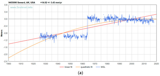
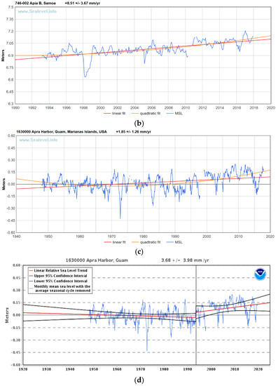
Figure 1.
Sample segmented tide gauge records available in databases of tide gauges. MSL (mean sea levels) of Seward (a), Apia B (b), Guam (c,d). Images (a) to (c) are reproduced and modified from www.sealevel.info. Image (d) is reproduced and modified from tidesandcurrents.noaa.gov.
In Figure 1a is the MSL of Seward, AK, with no correction introduced to account for an earthquake in the mid-1960s that moved up the instrument. The correct rate of rise [16] is −0.11 mm/yr pre-earthquake, and −1.74 mm/yr post-earthquake. The image suggests above +14 mm/yr of the rate of rise. This issue has been now corrected in the PSMSL database.
In Figure 1b is the MSL of Apia B, Samoa. The effect of the earthquake of 2011, shown by [7], is still unaccounted for in the PSMSL database. [7] revealed that the high rate of rise and high acceleration are only artifacts of the crustal movement connected to the earthquake. The almost +9 mm/yr sea level rate of rise is still used as proof that the sea level is rising faster in the Pacific Islands. This rate of rise practically vanishes to zero when the crustal motion is accounted for.
Figure 1c,d shows the MSL of Guam. The effect of two earthquakes is clear—one in the early 1990s, the other, which was much larger, at the end of the 1990s. However, NOAA placed a breakpoint about the first earthquake, the one with minor effects, and forgot the second one. By considering the short record starting from the time of the first earthquake, and ignoring the effect of the second earthquake, NOAA claim for Guam prior to the first earthquake a −1.05 mm/yr sea level rate of rise, and post the first earthquake a +8.58 mm/yr. [16]. This is also almost +9 mm/yr. The sea level rate of rise has been used as proof the sea levels are accelerating. Accounting for the effect of both earthquakes, the sea levels of Guam are also stable, as shown in [17].
Figure 1 explains how the problem of segmented records is widespread, also affecting records originated by the same tide gauge in the same location.
The aim of this work is to use breakpoints alignment techniques like those adopted for the global positioning system (GPS) time series [18,19,20] to detect suspicious alignments of segmented tide gauge records. Data mining and consistency with complete non-segmented tide gauge records are also used to address the misalignment issues. The case study selected to test the procedure is the Indian Ocean.
2. Materials and Methods
Two regressions are usually applied to the measured monthly average mean sea levels (MSL) of a tide gauge record to compute the sea level rate of rise and the acceleration. A linear regression:
returns the sea level rate of rise as the slope M. A quadratic regression:
returns the acceleration as twice the second-order coefficient 2·A. These computations are not reliable if the tide gauge record is segmented.
While the issue of different sea and land contributions moving from one tide gauge location to the other, or other biases to the tide gauge results originating from malfunctioning of the instrument or measurement errors, could not be addressed, there was the opportunity to verify if the alignments of the different segments satisfied some conditions, such as breakpoint alignments assuming a known pattern—for example, linear—across the segments, and extrapolate the values at the interface from both sides [2,3,21]. Regarding breakpoints detection in oceanic environmental variables, the reader is also referred to [22]. If there are n segments, the segmented time series is given as:
where yk(x) are the measurements collected by the tide gauge k, and δk is the shift that is applied to these measurements to produce a single time series. If n is the number of segments, there are (n − 1) relative shifts δi, i+1 for i = 1, n − 1 that must be verified. The number of segments composing the record was sometimes shown by comparing the PSMSL (www.psmsl.org) metric data, the raw data that the PSMSL stores before trying their alignment in their revised local reference (RLR) data set, with this latter result. Some other times, unfortunately, there was no information in PSMSL that a tide gauge record may be segmented. The databases considered for sea level information were PSMSL (www.psmsl.org) and NOAA (tidesandcurrents.noaa.gov). Supporting sea level analyses were sourced from sealevel.info (www.sealevel.info) as well as NOAA (tidesandcurrents.noaa.gov). Subsidence data were sourced from SONEL (www.sonel.org), JPL (sideshow.jpl.nasa.gov/post/series.html), and Nevada Geodetic Lab (geodesy.unr.edu).
The breakpoint alignment method alone fails to cover the option of legitimate changes in the trends, such as [22], that may occur during periods with missing values. This is the reason why the similarity between sea level patterns in the records from different tide gauges of the same ocean basin was sought. The breakpoint alignment method alone could not address the issues of the missing information periods in the records of Aden, Mumbai, or Karachi taken individually. The breakpoint alignment method coupled with the similarity analysis of the patterns between the sea levels of Aden, Mumbai, Karachi, and Fremantle could better address the issue, without being free of criticism. There is no fully satisfactory procedure that can overcome the issue of missing measurements, malfunction of instruments, or other perturbing issues. The suggestion is to flag the segmented tide gauge records as having quality issues and avoid computing any trend with these records.
3. Results
The Indian Ocean has four long-term trend tide gauges, three of which are segmented. An example of a segmented tide gauge record is Aden, where data have been collected over 135 years in five segments, with gaps totaling 67 years, by using different tide gauges [21]. Mumbai [2] and Karachi [3] are other remarkable examples of segmented tide gauge records. In Mumbai, data have been collected in five segments over 134 years, with gaps totaling 12 years, by using different tide gauges. In Karachi, data have been collected in four segments over 99 years, with gaps totaling 43 years, by using different tide gauges. There are concerns for the alignment of all the different segments of the three composite tide gauge records of Aden, Mumbai, and Karachi because the trends within the individual segments are mostly stable, and it is only their composition that produces a positive slope [2,3,21]. The present contribution proposes a procedure to check the alignment of segments when there is doubt about their misalignment.
Figure 2 presents a satellite view of the Indian Ocean, with the location of the Fremantle and Mumbai tide gauges indicated with an arrow. The figure also presents the main warm and cold currents for the area.
Figure 2.
(a) Satellite image of the ocean basin under study. Image reproduced and modified from www.psmsl.org/products/trends/. Warm and cold major currents for the area. (b) Image reproduced and modified from https://en.wikipedia.org/wiki/Ocean_current#/media/File:Corrientes-oceanicas.png.
Figure 3 presents the MSL of Aden, Mumbai, and Karachi. The figure also presents the MSL of Fremantle, the other long-term tide gauge of the Indian Ocean. Opposite to Aden, Mumbai, and Karachi, Fremantle is not a segmented record. In the pictures, from sealevel.info (www.sealevel.info), the MSL is claimed to be clear of the regular seasonal fluctuations due to coastal ocean temperatures, salinities, winds, atmospheric pressures, and ocean currents. The clearing process includes quite complicated operations that might be doubted, however marginally affecting the computed trends. Figure 3a,b presents the MSL for Aden, with data from NOAA (tidesandcurrents.noaa.gov/) and from PSMSL. The data from NOAA are simply an earlier version of the PSMSL data. The earlier version still available from NOAA is called (n − 1), and the latest version from PSMSL is called (n). As the databases of climate parameters are unfortunately unstable, it is common to have historical data revised from one version to the other.
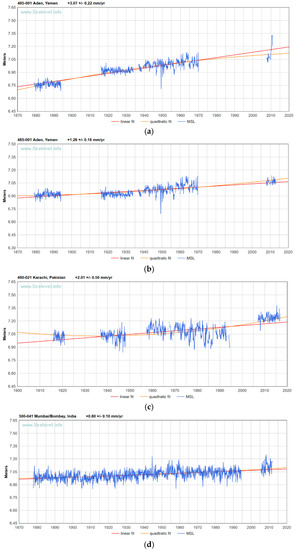
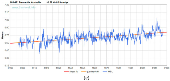
Figure 3.
Aden MSL results. (a) Version (n − 1), data sources are 795 months from the National Oceanic and Atmospheric Administration (NOAA). (b) Version (n), data source 815 months from Permanent Service for Mean Sea Level (PSMSL). Mumbai MSL results. (c) Data source 1465 months from PSMSL. Karachi MSL results. (d) Data source 673 months from PSMSL. Fremantle MSL results. (e) Data source 1331 months from PSMSL.
From a summary examination, the record for Aden includes two major gaps and one short gap. In Aden version (n − 1), Figure 3a, with the date range March 1879 to December 2010, the slope is 3.067 ± 0.222 mm/yr and the acceleration is −0.0237 ± 0.0099 mm/yr2 (negative). In Aden version (n), Figure 3b, with date range March 1879 to October 2013, the slope is +1.258 ± 0.156 mm/yr, and the acceleration is +0.01478 ± 0.00668 mm/yr2 (positive). Figure 3c presents the MSL for Mumbai. From a summary examination, it includes one gap. With the date range January 1878 to November 2011, the slope is +0.796 ± 0.095 mm/yr and the acceleration is +0.00664 ± 0.00538 mm/yr2. Figure 3d presents the MSL for Karachi. From a summary examination, it includes three gaps. With the date range January 1916 to December 2014, the slope is +1.850 ± 0.519 mm/yr and the acceleration is +0.0584 ± 0.0324 mm/yr2. Figure 3e presents the MSL for Fremantle. There are no gaps in this record. With the date range January 1897 to December 2016, the slope is +1.694 ± 0.246 mm/yr and the acceleration is +0.00571 ± 0.01567 mm/yr2.
In the case of Aden, one segment, the first of five, shifted down first, then up again 150 mm, for a misinterpretation of the published information about the tide gauges [21]. Over seven years, PSMSL has provided three different versions of the composite record of Aden, resulting in a strongly variable sea level rate of rise and acceleration. The historical data from 1879 to 1893 were first shifted down 150 mm, thus producing a much larger slope, but also a negative acceleration. Then, these data were shifted up again 150 mm, to produce a smaller slope, but a positive acceleration.
The PSMSL pattern (n − 2) of 2007 [23,24] suggested a slope for Aden of +1.21 mm/yr with data from 1880 to 1969. The PSMSL pattern (n − 1), valid up to about 2013, with a data range March 1879 to December 2010, suggested a slope of +3.067 ± 0.222 mm/yr, and acceleration −0.0237 ± 0.0099 mm/yr2 [21]. The PSMSL pattern (n) was then corrected only because of the large negative acceleration. As written in [25], “this resolves the anomalous negative acceleration value derived from the previous uncorrected data”. With dates ranging from March 1879 to December 2010, the slope is +1.330 ± 0.193 mm/yr and the acceleration is +0.0241 ± 0.0085 mm/yr2, a similar module but opposite sign. The rates of rise and accelerations have dramatically changed three times over a decade.
In the case of Aden, the alignment of the first segment in particular, but also the alignment of the last segment, appears questionable. As the network of benchmarks was compromised at the time the new tide gauge was set up, after a gap of 40 years from the prior measurements [21,26], the alignment of the new tide gauge was quite complicated. The Technical Survey [26] provided a clear description of the different tide gauges around Aden and the issues with the benchmarks: “The Great Triangulation Survey of India (GTS) provided various benchmarks around Tawahi Port of Aden”. However, “The primary benchmark at Fairway House/Post Office House next to Post Office Pier no longer exists and the other remaining vertical benchmark is at the North-East corner of the Port Engineers Office (PEO). There is another benchmark at the Pilots Pier tide gauge hut, situated on the lower wall by the steps next to the tide staff. Both benchmarks are in poor condition and need urgent repairs or replacing”. [26] concluded, “Re-establishing a new network of benchmarks should be a priority”.
Even though the Great Triangulation Survey of India (GTS) provided various benchmarks around Aden to align with the tide gauges of the time, nevertheless PSMSL made a mistake of 150 mm, misaligning the first segment with the others. Then, as the benchmarks were lost at the time the new tide gauge was set up, it is unclear how the alignment of the new tide gauge could have been performed with accuracy.
In the case of Aden, but also Mumbai and Karachi, the last segments, from the new, recently established tide gauges, which were started almost simultaneously in the three locations as part of a common international monitoring project, are very likely all misaligned with the prior segments from the historical tide gauges after substantial gaps in the measurements [2,3,21].
The procedure outlined in the Method section was applied to the tide gauge records of Aden, Mumbai, and Karachi. The different segments were detected first. Then, the breakpoint alignment was attempted. Finally, consistency with the Fremantle tide gauge record was tested.
3.1. Aden
The tide gauge record of Aden was analyzed in [21]. Figure 4 presents the RLR (revised local reference) and MET (metric) data of PSMSL (data downloaded from www.psmsl.org/data/obtaining/rlr.monthly.data/44.rlrdata, www.psmsl.org/data/obtaining/met.monthly.data/44.metdata, accessed on 18 May 2018), plus their difference Delta RLR-Met. As the database is unstable (see Figure 3), the date of download is important.
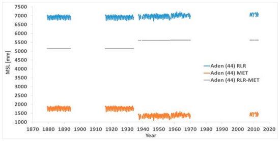
Figure 4.
PSMSL RLR (revised local reference) and MET (metric) data for Aden, plus their difference Delta RLR-Met. There were five segments, with four offsets to verify.
The different segments were found from either a change of the Delta RLR-Met, significant gaps without measurements, or specific mention in the station documentation from PSMSL.
The station documentation from PSMSL is insufficient. It does not report changes in tide gauges. It is written:
- −
- 1937–1956 values based on high and low water readings;
- −
- Aden 485/001 RLR (1962) is 9.1 m below BM PEO;
- −
- 2007/8 one-minute sea level data downloaded from the IOC Sea Level Station Monitoring Facility Ostend. This is then converted to 15 min data for processing. 2008 monthly and annual mean sea level values have now been extracted from the data. As the relationship for the prime benchmark remains the same there is no need to alter RLR. Details of the benchmarks have been derived from site installation information. Copies of these have been included in the port files and RLR file for reference;
- −
- The historic data for Aden (1879–1933) have been reviewed. As a result, the RLR factor for all that period has been set to 5.141 m;
- −
- A value of MTL − MSL = 16 mm has been applied to the RLR data for the period 1937–1956 using harmonic constituents from the GESLA2 (high-frequency tide gauge) dataset.
The data for Aden showed five (5) sets of measurements, 1879 to 1893, 1916 to 1933, 1937 to 1956, 1957 to 1969 and 2007 to present.
After having found the different segments, their alignment was then checked. A known pattern across the segment must be assumed. The simplest pattern is linear. As the length of the segments is usually short, polynomials do not work better. In the case of two segments of equal length, a breakpoint is placed at the center of the gap between two segments, while in the case of two segments of unequal length, the breakpoint is placed closer to the shortest segment. An offset in between the two segments is computed with the same values at the breakpoint from the left and right extrapolations.
Figure 5a,b presents the latest Aden results, data from March 1879 to October 2013. Figure 5a shows the linear fittings applied to the five segments. Figure 5b shows the MSL aligned compared to the PSMSL RLR data. In none of the five segments, was there a rate of rise approaching the rate of rise of the segmented record proposed by PSMSL.
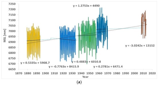
Figure 5.
Aden results. (a) Linear fittings applied to the five segments. (b) MSL aligned compared to the PSMSL RLR data. (c) MSL aligned, with the same method, but only three segments, as in [21], with the latest data omitted, compared to the PSMSL RLR data. When measured, the sea levels are rising slowly, or they are decreasing. The rising trend of the PSMSL RLR data is the result of the shifts of one segment versus the other, always upwards versus the values suggested by the alignment of the breakpoints.
In the PSMSL RLR data, the sea levels were rising at a rate of +1.28 mm/yr. In none of the segments were the sea levels are rising at such a rate. The mean trend through all segments (Figure 5a) supplied an elusive rate not anchored in observational records. We may even say that such a record must be discarded as improper. The rates were +0.53 mm/yr in segment 1, −0.78 mm/yr in segment 2, +0.49 mm/yr in segment 3, +0.28 mm/yr in segment 4, and finally −3.02 mm/yr in segment 5. This one is by far too short. The rising trend of the PSMSL RLR data is the result of the shifts of one segment versus the other, always upwards versus the values suggested by the alignment of the breakpoints.
In the realignment, segment 2 was shifted down 10.7 mm versus segment 1. Segment 3 was shifted down 42.6 mm versus segment 2. Segment 4 was shifted down 49.2 mm versus segment 3. Segment 5 was shifted down 50.3 mm versus segment 4. The slope was thus reduced from +1.28 to +0.02 mm/yr. The acceleration was also reduced from +0.0164 to +0.0038 mm/yr2.
Comparable results were obtained by [21], however no correction was introduced for the data of 1879 to 1893 and 1916 to 1933, which were aligned on their own in the metric version. Additionally, the data from 2007 to 2013 were neglected in [21], as they are 6 years of data after a gap of 40 years. [21] only aligned three segments, 1879 to 1933, 1937 to 1956, 1957 to 1969. They resolved the alignment of the first two segments with the same breakpoint alignment, and of the second and third, just a few months, with either the same breakpoint alignment or similarity to Mumbai.
With reference to Figure 5a, segment 3 was shifted down 30 mm versus segments 1 and 2, and segment 4 was shifted down 50 mm versus segment 3. The sea level trend 1879 to 1969 of [21] was +0.24 mm/yr.
From Figure 5 it may be only concluded that the alignments used by the PSMSL are not trustworthy, and the rate of rise of the sea levels is much smaller than the alleged +1.28 mm/yr, more likely completely de-trended or only weakly rising. Therefore, we feel that there is an urgent need to break down the tide-gauge record into a detailed analysis of the five segments independently.
3.2. Karachi
The tide gauge of Karachi was analyzed in [3]. Figure 6 presents the RLR (revised local reference) and MET (metric) data of PSMSL for Karachi (data downloaded from www.psmsl.org/data/obtaining/rlr.monthly.data/204.rlrdata, www.psmsl.org/data/obtaining/met.monthly.data/204.metdata, accessed on 18 May 2018), plus their difference Delta RLR-Met. The different segments are clearly shown from either change in the Delta RLR-Met or significant gaps without measurements.
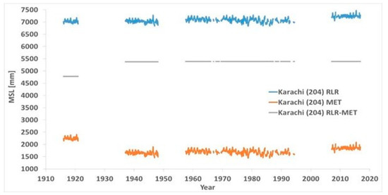
Figure 6.
PSMSL RLR and MET data for Karachi, and their difference Delta RLR-Met. There are four segments, with three offsets to verify.
The station documentation from PSMSL reports:
- −
- Bombay (Apollo B) 500/041 RLR (1964) is 13.0 m below BM 2(PP);
- −
- 1931–1958 values based on readings of high and low waters;
- −
- Benchmark and datum details for 2005/6 remain the same as previously, so the same RLRFAC (RLRFAC is the Revised Local Reference factor for the station-year) was used;
- −
- Benchmark for the historical data up to 1965 was BM 2PP1, up to 1936 the datum was 9.132 m below this benchmark;
- −
- For data 1937 onwards, the datum was “Chart Datum” with BM 2PP1 being 8.522 m above this;
- −
- In 1966 the benchmark was changed to BM 5/88 7.44 m above chart datum;
- −
- Please note that the monthly mean sea level values for the period 1931 to 1936 were reported only to the nearest tenth of a foot, approximately 30 mm. This explains the appearance of discrete sampling in height of the sea level variation during this time;
- −
- We changed the first line above, indicating that the MTL ended in 1958, not 1956 as was previously stated. We verified that the values in the database are those from PubSci 20, in which they were indicated as MTL;
- −
- A value of MTL − MSL = 31 mm was applied to the RLR data for the period 1931–1958. This value was derived from the average of three differences in the annual MSL and MTL listed in PubSci 24. Note that no correction was applied to the metric data.
The data for Karachi show four (4) sets of misaligned measurements, 1916 to 1920, 1937 to 1948, 1957 to 1995, and 2007 to present.
Figure 7a,b presents the latest Karachi results, data from January 1916 to November 2016. Figure 6a shows the linear fittings applied to the four segments. Figure 6b shows the MSL aligned compared to the PSMSL RLR data.
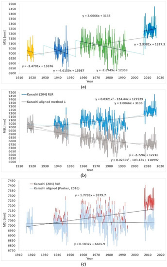
Figure 7.
Karachi. (a) Linear fittings applied to the four segments. (b) MSL aligned compared to the PSMSL RLR data. (c) MSL aligned with the same method, but only three segments, as in [3], compared to the PSMSL RLR data. When measured, the sea levels were decreasing. The rising trend of the PSMSL RLR data is the result of the shifts of one segment versus the other, always upwards versus the values suggested by the alignment of the breakpoints.
When measured, the sea levels were decreasing, apart from the last segment.
In the PSMSL RLR data, the sea levels were rising at a rate of +2.01 mm/yr. In none of the segments were the sea levels rising at such a rate, except the noticeably short segment 4. The rates were −3.47 mm/yr in segment 1, that was too short, −4.62 mm/yr in segment 2, −2.67 mm/yr in segment 3, and finally +2.94 mm/yr in segment 4, that was too short.
The rising trend of the PSMSL RLR data is the result of the shifts of one segment versus the other, always upwards versus the values suggested by the alignment of the breakpoints. In the realignment, segment 2 was shifted down 99.7 mm versus segment 1. Segment 3 was shifted down 164.2 mm versus segment 2. Segment 4 was shifted down 213.9 mm versus segment 3. The slope was thus reduced from +2.01 to −2.73 mm/yr. The acceleration was also slightly reduced from +0.0642 to +0.0510 mm/yr2.
Figure 7a gives an expressive example of how serious analyses of meaningful sea level trends must never use data recorded by tide-gauges. It shows an almost shocking misuse of available data.
Comparable results were obtained by [3], however no correction was introduced for the data of 1937 to 1948 versus 1957 to 1995, which was then considered a single segment. This study only aligned three segments, 1916 to 1920, 1937 to 1995, and 2007 to 2015 [3]. The alignment of the first two segments, and of the last two, was resolved with the same breakpoint alignment. With reference to Figure 7a, segment 2 and segment 3 were shifted down 37.5 mm versus segment 1, and segment 4 was shifted down 161.6 mm versus segment 3. With data from January 1916 to December 2014, the sea level trend of [3] was +0.18 mm/yr versus +1.78 mm/yr of the PSMSL RLR, Figure 7c.
From Figure 7 it may be only concluded that the alignments used by the PSMSL are not trustworthy, and the rate of rise of the sea levels was much smaller than the alleged +2.01 mm/yr, more likely weakly reducing rather than rising.
3.3. Mumbai
The tide gauge of Mumbai was analyzed in [2] and discussed with respect to independent coastal morphological criteria [27]. Figure 8 presents the RLR (revised local reference) and MET (metric) data of PSMSL for Mumbai (data downloaded from www.psmsl.org/data/obtaining/rlr.monthly.data/43.rlrdata, www.psmsl.org/data/obtaining/met.monthly.data/43.metdata, accessed on 18 May 2018), plus their difference Delta RLR-Met. The different segments are clearly shown from either change in the Delta RLR-Met or significant gaps without measurements.
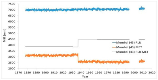
Figure 8.
PSMSL RLR and MET data for Mumbai, and their difference Delta RLR-Met. There were five segments, with four offsets to verify.
The station documentation from PSMSL is insufficient. It does not report changes in tide gauges. It is written that:
- −
- Anomalously large value June 1946 and low values at end of 1946 (just before a data gap)—correct as received from authority;
- −
- Data for 1916–1920 are MSL and were obtained from the Survey of India, Dehra Dun;
- −
- Data for 1937–1948 are MTL (Mean Tide Level) and were also obtained from the Survey of India;
- −
- Data from 1957 onwards are MSL;
- −
- Data from 1957–1965 were obtained from the Pakistan Meteorological Department, while 1966–1985 from National Institute of Oceanography. Data from 1986–1987 were obtained from the University of Hawaii Sea Level Center using data supplied by the NIO (National Institute of Oceanography);
- −
- Karachi 490/021 RLR (1947) is 9.7 m below BM 1PP (circa 1920);
- −
- New data from the Pakistan Navy for 1987 replace TOGA (Tropical Ocean and Global Atmosphere programme) data for Jan–Apr and Dec;
- −
- The gauge at Karachi has been re-sited and is now no longer on Manora Island. The new gauge has been leveled into the old one. One-minute sea level data from 2007/2008 were downloaded from the IOC Sea Level Station Monitoring Facility Ostend. This was then converted to 15 min. data for processing. Monthly and annual mean sea level values from 2007/2008 were then extracted from the data. As the relationship for the prime benchmark remains the same there is no need to alter RLR. Details of the benchmarks have been derived from site installation information. Copies of these have been included in the port files and RLR file for reference;
- −
- A value of MTL – MSL = 10 mm was applied to the RLR data for the period 1937–1948. Values were derived using values from the GESLA2 (high-frequency tide gauge) dataset. A value of 10 mm was used from the historic databank of harmonic tidal constants gathered by the International Hydrographic Organization.
The data for Mumbai showed five (5) sets of misaligned measurements, 1878 to 1930, 1931 to 1936, 1937 to 1958, 1959 to 1994, and 2007 to present.
Figure 9a,b presents the latest Mumbai results, data January 1878 to October 2011. Figure 9a shows the linear fittings applied to the five segments. Figure 9b shows the MSL aligned compared to the PSMSL RLR data. When measured, the sea levels were decreasing, apart from the last segment. In the PSMSL RLR data, the sea levels were rising at a rate of +0.80 mm/yr (+0.77 mm/yr according to [24]. In two of the five segments, the sea levels were rising at about that rate, but in the remaining three segments, they were rising at a much smaller rate, or even decreasing. The rates were +0.15 mm/yr in segment 1, −6.73 mm/yr in the noticeably short segment 2, +0.98 mm/yr in segment 3, −0.16 mm/yr in segment 4, and finally +7.67 mm/yr in the short segment 5. The longest segments, segment 1 and segment 4, had very stable sea levels, +0.15 mm/yr and −0.16 mm/yr.
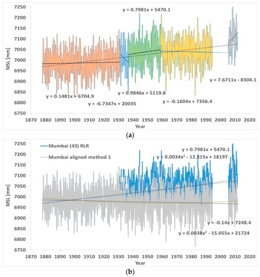
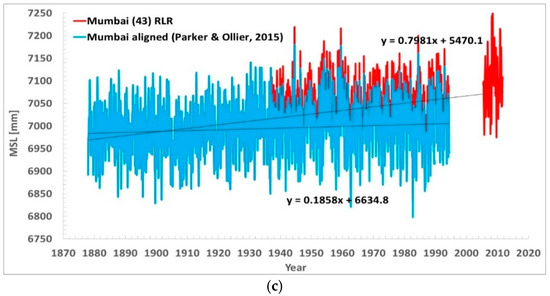
Figure 9.
Mumbai. (a) Linear fittings applied to the five segments. (b) MSL aligned compared to the PSMSL RLR data. (c) MSL aligned the same method, but only three segments, as in [2,21], compared to the PSMSL RLR data. When measured, the sea levels were decreasing. The rising trend of the PSMSL RLR data was the result of the shifts of one segment versus the other, always upwards versus the values suggested by the alignment of the breakpoints.
The rising trend of the PSMSL RLR data is the result of the shifts of one segment versus the other, always upwards versus the values suggested by the alignment of the breakpoints.
In the realignment, segment 2 was shifted down 38.8 mm versus segment 1. Segment 3 was shifted down 37.3 mm versus segment 2. Segment 4 was shifted up 6.5 mm versus segment 3. Segment 5 was shifted down 45.3 mm versus segment 4. The slope was thus reduced from +0.80 to −0.14 mm/yr. The acceleration was now slightly increased from +0.0068 to +0.0076 mm/yr2.
Comparable results were obtained by [2,21], however only two segments were considered, 1878 to 1936 and 1937 to 1994, while the latest data were neglected. The alignment of the two segments was resolved with the same breakpoint alignment.
With reference to Figure 9a, segment 3 and segment 4 were shifted down 38.8 mm versus segments 1 and 2. With data from January 1878 to June 1994, the sea level trend of [2] was +0.19 mm/yr versus the +0.80 mm/yr of the PSMSL RLR, Figure 9c.
From Figure 9, it may be concluded that, despite less evident than in the case of Aden and Karachi, the alignments operated by the PSMSL are not trustworthy, and the rate of rise of the sea levels is certainly smaller than the alleged +0.80 mm/yr, more likely only slightly positive, in good agreement with the shore morphological analysis of [27,28]. A combination with shore morphology and shore stratigraphy offers a means of overcoming the problems and reconstructing past sea levels in a meaningful way [27,28].
3.4. Comparison with Fremantle
Figure 4, Figure 5, Figure 6, Figure 7, Figure 8 and Figure 9 prove that some of the alignments proposed by the PSMSL are likely incorrect. They are producing rising and accelerating trends in composing segments where the sea level is not rising. However, the proposed method did not make it possible to produce a reliable time series to be used to compute the sea level rate of rise and acceleration. If the measurements for the past were not taken properly—in the same location, with the same tide gauge, continuously—there is no opportunity to reconstruct a reliable time series. While different alignment techniques may certainly be proposed, all these works will remain subjective reanalyses of segments in a record, which are impossible to couple together to form a reliable individual time series.
From Figure 4, Figure 5, Figure 6, Figure 7, Figure 8 and Figure 9, it is possible to claim that it is more likely that the sea levels have been mostly stable in Aden, Mumbai, and Karachi, rather than rising at the rates and accelerations proposed by the PSMSL RLR data. Especially for Aden and Karachi, the rates of rise and the accelerations were certainly overrated in the PSMSL RLR data. However, there was no opportunity to know with accuracy the precise values of sea level rate of rise and acceleration.
Long-term segmented tide gauges should be compared with long-term non-segmented tide gauges in the same basin to discover differences. We considered the tide gauge of Fremantle, in Australia, the best tide gauge of the Indian Ocean [29], Figure 10. The PSMSL RLR data downloaded from www.psmsl.org/data/obtaining/stations/111.php on 6 June 2018, with date range January 1897 to December 2016, suggest a relative rate of rise of +1.67 mm/yr and acceleration of +0.006 mm/yr2. The completeness of the tide gauge is 92%. By filling the gaps interpolating the data from the same month in neighboring years, the relative rate of rise becomes +1.70 mm/yr and the acceleration +0.005 mm/yr2.
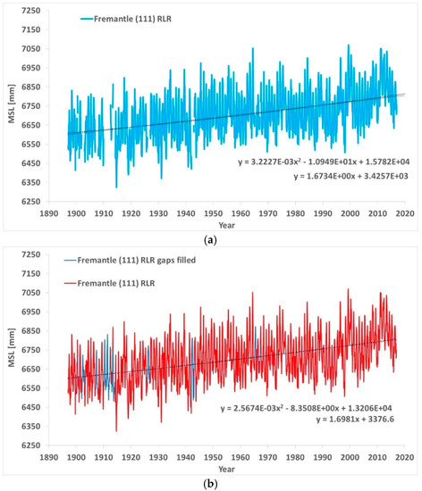
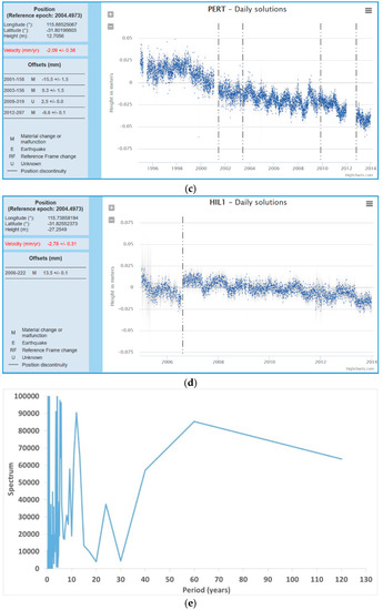
Figure 10.
Fremantle. (a) and (b) linear and parabolic fittings of the PSMSL RLR data, as it is or with gaps filled. (c) and (d) subsidence rates of nearby GPS domes. Images reproduced and modified from SONEL, www.sonel.org. (e) Periodogram of the PSMSL RLR data with gaps filled about the parabolic trend.
The rate of rise of the sea level is less than the subsidence rate of the nearby GPS dome of PERT (in Landsdale). According to SONEL (www.sonel.org), the subsidence rate of this inland dome is −2.09 ± 0.38 mm/yr. Even larger subsidence was found by SONEL for the similarly close inland GPS dome of HIL1 (in Hillarys). The subsidence rate here is here −2.78 ± 0.31 mm/yr.
According to JPL (sideshow.jpl.nasa.gov/post/series.html), the subsidence rate for PERT (in Landsdale) is −2.883 ± 0.612 mm/yr. While the Fremantle tide gauge may be subjected to reduced subsidence compared to the GPS domes of PERT (in Landsdale) or HIL1 (in Hillarys), certainly all the Perth basin is subjected to subsidence [30,31].
Nevada Geodetic Lab (geodesy.unr.edu) has many more GPS antennas in the area. PERT (in Landsdale) has a subsidence rate of −1.933 ± 0.603 mm/yr; HIL1 (in Hillarys) has a subsidence rate of −2.821 ± 0.603 mm/yr. Moving closer to the tide gauge location, WLT1 (in Willetton) has a subsidence rate of −3.821 ± 1.231 mm/yr, CUTA and SPA8, both slightly south of East Victoria Park, about the location of Curtin University, have a subsidence rate of −1.108 ± 0.944 mm/yr, and–3.795 ± 1.529 mm/yr. respectively.
Both the MSL and the GPS position results from SONEL are shown in Figure 10. The figure also presents the periodogram of the oscillations about the parabolic trend, for the case of the PSMSL RLR with gaps filled. The periodogram clearly shows a 60-years periodicity, as well as a 13-years periodicity. Then, there is another, but smaller, periodicity of about 24 years. Similar oscillations are expected in Aden, Karachi, and Mumbai.
Trends like Fremantle, where the absolute sea levels are not rising, are expected in Aden, Mumbai, and Karachi, where a lack of subsidence may translate to a lack of sea level rise. Recent past subsidence of parts of the Perth Basin has most probably been caused by increased groundwater extraction for domestic and agricultural use [30,31]. This may explain the positive sea level acceleration of Fremantle, rated at +0.00571 mm/yr2.
Compared to Fremantle, the acceleration of Aden is a huge +0.0164 mm/yr2 in the PSMSL RLR data and it is +0.0038 mm/yr2 in the data realigned. The acceleration of Karachi is a huge +0.0642 mm/yr2 in the PSMSL RLR data and it is still exceptionally large at +0.0510 mm/yr2 in the data realigned. The acceleration in Mumbai is +0.0068 mm/yr2 in the PSMSL RLR data and it is +0.0076 mm/yr2 in the data realigned.
Figure 11 presents a comparison of the MSL of Fremantle and Aden (a) and their differences (b), plus a comparison of the MSL of Fremantle and Karachi (c) and their differences (d).
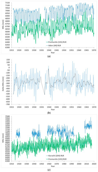
Figure 11.
Comparison of the MSL of Fremantle and Aden (a) and their differences (b). Comparison of the MSL of Fremantle and Karachi (c) and their differences (d).
The offsets of the Aden segmented record 1933–1937 and 1956–1957 were tested for similarity with Fremantle. As Fremantle had the largest relative sea level rise, the difference in the MSL in Fremantle and Aden increased at a rate of 0.7065 mm/yr. At the offsets, in between 1933–1937, and in between 1956–1957, there were two suspicious “jumps” towards more negative values.
The offsets of the Karachi segmented record 1920–1937, 1948–1957, and 1995–2007, were tested for similarity with Fremantle. As Fremantle and Karachi had a close relative sea level rise, the difference in the MSL in Fremantle and Karachi was about constant (it only increased at a rate of 0.0987 mm/yr.). At the offsets between 1948–1957 and 1995–2007, there were two suspicious “jumps” towards more negative values.
The breakpoint alignment technique may be applied to the Fremantle tide gauge record, modified by introducing the gaps of Aden or Karachi (Mumbai is affected to a lesser extent by gaps). Figure 12 presents the analysis of the Fremantle MSL records, with the same gaps as Aden. With data from 1916 to 2013 (the common time window of the two tide gauges), there were four segments and three gaps to consider. The first three segments had in Aden a very close linear trend, from −0.78 to +0.49 mm/yr, which, considering the noticeably brief time windows of 18, 20, and 13 years, indicates the presence of small oscillations over these time windows. Also, the noticeably short last segment, less than a decade long, had a linear trend of −3.02 mm/yr. In the case of Fremantle, with the same gaps as Aden (Figure 12b), the difference in the trends for the first three segments was much larger, from +0.11 to +4.88 mm/yr, reflecting much larger oscillations over these time windows. The noticeably short last segment of trend +14.21 mm/yr confirms this impression. The breakpoint alignment technique may supply satisfactory results only in specific cases, where the segments are long enough, and there are no strong oscillations over the time window to bias the linear trends.
Figure 12.
MSL of Fremantle with the same gaps as Aden. (a) The effect of the gaps. (b) Breakpoints alignment. (c) Aligned series with gaps.
In the case of Fremantle with the introduced gaps of Aden, the breakpoint technique with assumptions of the break-points suggests an increase of the second segment versus the first of 44.9 mm, an increase of the third segment versus the second of 34.9 mm, and decrease of the fourth segment versus the third of 102.9 mm.
Over the time window 1916 to 2013, with all the data considered and no gaps, the sea level trend in Fremantle was +1.65 mm/yr, as seen in Figure 12a.
By simply introducing the gaps, the sea level trend increased to +2.27 mm/yr, Figure 12a. The simple presence of gaps makes the estimation non-accurate.
By applying the breakpoint alignment technique, detailed in Figure 12b, the aligned data suggest a trend of +2.45 mm/yr (Figure 12c), that is, an 8% difference.
Figure 13 presents the analysis of the Fremantle MSL records, with the same gaps as Karachi. The sea level oscillations appeared much stronger in Fremantle than Karachi. In Karachi, the first three segments all had negative trends, from −2.67 mm/yr (the longest segment) to −4.62 mm/yr (the intermediate segment). The first, shortest segment, less than a decade, had a linear trend of −3.47 mm/yr. The last segment, less than two decades long, had a linear trend of +2.93 mm/yr. In Fremantle, with the same gaps as Karachi (Figure 13b), the first segment had a huge negative trend of −23.49 mm/yr. The other segments had a linear trend variable between −1.85 and +3.86 mm/yr. The breakpoint technique with three gaps worked poorly, suggesting a decrease in the second segment compared to the first of 46.5 mm, a decrease in the third segment compared to the second of 5.7 mm, and a decrease in the fourth segment compared to the third of 117.5 mm.
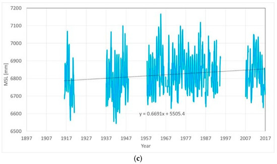
Figure 13.
MSL of Fremantle with the same gaps in Karachi. (a) The effect of the gaps. (b) Breakpoints alignments. (c) Aligned series with gaps.
Over the time window 1916 to 2017, with all the data considered, the sea level trend in Fremantle was +1.65 mm/yr, as seen Figure 13a.
By simply introducing the gaps, the sea level trend increased to +2.11 mm/yr. The simple presence of gaps makes the estimation inaccurate.
By applying the breakpoint alignment technique with three gaps, as seen in Figure 13b, the aligned data suggested a trend of +0.67 mm/yr, which is a significant difference.
The breakpoint alignment technique only works in specific conditions, when the trends for the different segments suffer from fewer oscillations. If this is not the case, the technique does not help. As there are usually interannual, decadal, and multidecadal oscillations up to 60 years, which can be very strong in the sea level signals, trends computed with only 10 or 20 years of data may be particularly misleading.
The best advice when there are segments is not to couple together the segments, that, at the most, can be analyzed only independently [1,5,6]. PSMSL, NOAA, and the other holders of tide gauge data, should simply quality flag all the tide gauges that are segmented.
4. Discussion
Long-term segmented tide gauges should also be compared for acceleration with the averages of long-term tide gauges in other basins to discover differences. As discussed in [21,32], the naïve average sea level rates of rise and acceleration of different data sets are characterized by small rates of rise and small accelerations despite the presence of many segmented records like Aden, Mumbai, and Karachi. The average trends and accelerations for these data sets are as follows:
- −
- +1.61 ± 0.21 mm/yr and +0.0020 ± 0.0173 mm/yr2 for the Mitrovica-23 data set;
- −
- +1.77 ± 0.17 mm/yr and +0.0029 ± 0.0118 mm/yr2 for the Holgate-9 data set;
- −
- +0.40 ± 0.27 mm/yr and +0.0090 ± 0.0208 mm/yr2 for the NOAA-120 data set;
- −
- +1.63 ± 0.23 mm/yr and +0.0021 ± 0.0192 mm/yr2 for the US 39 data set;
- −
- +0.49 ± 0.34 mm/yr and +0.0063 ± 0.0263 mm/yr2 for the PSMSL-162 data set;
- −
- +1.19 ± 0.29 mm/yr and +0.0014 ± 0.0266 mm/yr2 for the California-8 data set.
The NOAA-120, PSMSL-162, and California-8 data sets have, on average, shorter lengths of tide gauge records. The naïve average global sea level acceleration is therefore in the order of +0.002 ÷ 0.003 mm/yr2.
The acceleration in Karachi is unrealistic, in both the PSMSL RLR and the realigned data.
The acceleration in Aden is also unrealistic in the PSMSL RLR data.
Reference to prior works is sometimes relevant to better understand the pattern of long-term segmented tide gauges. This is marginally the case of the three segmented records of Aden, Mumbai, and Karachi, that have not been at the center of many studies.
According to [33], the record for Mumbai between 1952 and 1962 completely reversed the entire rising trend for the previous 30 years. Based on the linear fitting of the MSL data, in the latest PSMSL RLR data set, the rate of rise from January 1932 to December 1961 was +1.56 mm/yr. When the data were realigned, it was +0.65 mm/yr. Opposite to Mumbai, [33] proposes more significant rising trends for Aden and Karachi.
According to [34], the sea level rate of rise in Mumbai over the time window 1930 to 1980 was a negative −0.30 mm/yr. Based on the linear fitting of the MSL data, in the latest PSMSL RLR data set, the rate of rise from January 1930 to December 1979 was +0.52 mm/yr. When the data were realigned, it was +0.08 mm/yr. Douglas did not include Aden and Karachi in his analysis [34].
In contrast to [34], other studies [33,35] computed a large sea level rate of rise for Mumbai, of +0.91 mm/yr over the time window 1878–1982. The differences [33,36] were attributed to, “somewhat different changes of mean annual land level (or relative sea level) obtained from the two sets of records to our generally earlier and later records”. Based on the linear fitting of the MSL data, in the latest PSMSL RLR data set, the rate of rise from January 1978 to December 1981 was +0.79 mm/yr. When the data were realigned, it was −0.24 mm/yr. Emery and Aubrey [35] did not include Aden and Karachi in their analysis.
More recent works, such as [2,3,21,23,24], have been previously mentioned.
In support of stable sea levels for the Indian Ocean, [27] proposed multiple lines of evidence, including coastal morphology, stratigraphy, radiocarbon dating, archaeological remains, historical documentation, and tide gauge records for Goa over the last 500 years. They evidenced an oscillatory pattern made up of a low water level in the early 16th century, a ~50 cm high level in the 17th century, a level below present sea level in the 18th century, a ~20 cm high level in the 19th and early 20th centuries, a ~20 cm fall in 1955–1962, and a virtually stable level over the last 50 years [27]. This sea level record is almost identical to those obtained in the Maldives [37,38] and in Bangladesh [1]. The Late Holocene sea level changes in the Maldives as described by [37] showed seven transgression peaks in the last 4000 years, with three peaks in the last millennium, and absolutely nothing unprecedented occurred during the last few decades. It was concluded that the Indian Ocean lacks any record of alarming sea level rise in recent decades [27].
While ocean and coastal management should certainly be based on proven sea level data [39], it is important to make sure the databases of tide gauge records do not have segmented records without quality flags. It is important that the many segmented tide gauge records in databases of tide gauges are quality flagged, as offering them as single quality records is misleading.
Opposite to the models, the results of the tide gauges show no sign of acceleration. The presence of segmented records in the databases has not much changed the small average rate of rise, and the negligible average acceleration, of the compilations of long-term-trend (LTT) tide gauges. However, there have been cases where segmented tide gauges have been wrongly used to support claims of dramatically rising and accelerating sea levels, in compliance with the model predictions.
It must be mentioned that databases of tide gauges such as NOAA and PSMSL include both segmented records and single tide gauge records. Sometimes, they also omit to consider some data of long-term-trend tide gauges of stable sea levels, such as Wajima and Hosojima [17].
The Geospatial Information Authority of Japan [40] has provided data of Hosojima since January 1894, Wajima since January 1894, and Oshoro since November 1905. Data are updated to early 2018. For Hosojima and Wajima, NOAA and PSMSL neglect the data collected prior to 1930. NOAA does not consider Oshoro at all, while PSMSL only considers the data since 1930 but split into two tide gauges, Oshoro and Oshoro II.
5. Conclusions
The databases of tide gauge records include many segmented records, where data originate from tide gauges having different sea and land contributions to the relative sea level signal, and the segments are misaligned, or suffer from other quality issues, such as earthquakes. These segmented records should not be considered as a single tide gauge record for assessing sea level rate of rise and acceleration. Many records in the PSMSL and NOAA database are segmented, and they should be quality flagged.
We proposed a simple technique to find alignment inaccuracies, by placing breakpoints in the gaps between every two segments and computing the relative offset between every two segments needing the same values at the breakpoint from left and right extrapolations, to test suspicious alignments. Applied to the records of Aden, Mumbai, and Karachi, the technique showed inaccuracies in the alignments of the different segments. Extremely worrying is the misalignment of the reading from the novel tide gauges, contemporarily set up in the three locations (as well as many other locations worldwide) about the year 2007, versus the reading of the historical tide gauges for the same locations.
While breakpoint techniques may be used to discover misalignments, their efficacy strongly varies from case to case, depending on the length of the segments and the phasing of the periodic oscillations. Segmented records should be quality flagged. No use should be made of records resulting from the composition of segments to infer sea level rates of rise or accelerations. If a tide gauge record has many gaps, there are doubtful alignments, it originates from different tide gauges, the record is affected by crustal movements such as earthquakes, the instrument has been damaged, the land below the tide gauge is subsiding, or it suffers from other quality issues, it should not be considered a single quality record, but quality flagged and disregarded for the purpose of computing rates of rise and accelerations over the full time of the record. There is a clear need for quality assurances for all the data sets that serve the purpose of supplying vital information to policymakers. The more reliable the data sets, the better the policy that can be based on these data.
Author Contributions
This is a single author contribution. All authors have read and agreed to the published version of the manuscript.
Funding
This research received no external funding.
Conflicts of Interest
The author declares no conflict of interest.
References
- Mörner, N.A. Sea level changes in Bangladesh new observational facts. Energy Environ. 2010, 21, 235–249. [Google Scholar] [CrossRef]
- Parker, A.; Ollier, C.D. Sea level rise for India since the start of tide gauge records. Arab. J. Geosci. 2015, 8, 6483–6495. [Google Scholar] [CrossRef]
- Parker, A. Analysis of sea level in Karachi. New Concepts Glob. Tecton. 2016, 4, 1201–1226. [Google Scholar]
- Parker, A.; O’Sullivan, J. The Need of an Open, Fair Peer Review of Sea Levels Data. New Concepts Glob. Tecton. J. 2018, 6, 231–252. [Google Scholar]
- Mörner, N.A.; Matlack-Kein, P. The Fiji tide-gauge stations. Int. J. Geosci. 2017, 8, 536. [Google Scholar] [CrossRef][Green Version]
- Mörner, N.A.; Matlack-Klein, P. New records of sea level changes in the Fiji Islands. Oceanogr. Fish. Open Access J. 2017, 5, 20. [Google Scholar] [CrossRef]
- Parker, A.; Mörner, N.; Matlack-Klein, P. Sea level acceleration caused by earthquake induced subsidence in the samoa islands. Ocean. Coast. Manag. 2018, 161, 11–19. [Google Scholar] [CrossRef]
- Chambers, D.; Merrifield, M.A.; Nerem, R.S. Is there a 60-year oscillation in global mean sea level? Geophys. Res. Lett. 2012, 39. [Google Scholar] [CrossRef]
- Iyengar, R.N. Monsoon rainfall cycles as depicted in ancient Sanskrit texts. Curr. Sci. 2009, 97, 444–447. [Google Scholar]
- Schlesinger, M.; Ramankutty, N. An oscillation in the global climate system of period 657–0 years. Nature 1994, 367, 723. [Google Scholar] [CrossRef]
- Scafetta, N. The complex planetary synchronization structure of the solar system. Pattern Recognit. Phys. 2014, 2, 1–19. [Google Scholar] [CrossRef]
- Mörner, N.A. Soar wind, Earth’s rotation and changes in terrestrial climate. Phys. Rev. Res. Int. 2013, 3, 117–136. [Google Scholar]
- Mörner, N.A. Multiple planetary influence on the Earth. In Planetary Influence on the Sun and the Earth, and a Sad Modern Book-Burning; Mörner, N.A., Ed.; Nova Science Publishers: Hauppauge, NY, USA, 2015. [Google Scholar]
- Mörner, N.A. Sea level changes past records and future expectations. Energy Environ. 2013, 24, 509–536. [Google Scholar] [CrossRef]
- Telesca, L.; Lovallo, M.; Pierini, J.O. Visibility graph approach to the analysis of ocean tidal records. Chaos Solitons Fractals 2012, 45, 1086–1091. [Google Scholar] [CrossRef]
- Zervas, C.E. Sea Level Variations of the United States; Technical Report NOS CO-OPS 053; NOAA: Silver Spring, MD, USA, 2009. [Google Scholar]
- Parker, A. Sea level oscillations in Japan and China since the start of the 20th century and consequences for coastal management-Part 1: Japan. Ocean. Coast. Manag. 2019, 169, 225–238. [Google Scholar] [CrossRef]
- Blewitt, G. An automatic editing algorithm for GPS data. Geophys. Res. Lett. 1990, 17, 199–202. [Google Scholar] [CrossRef]
- Blewitt, G. Carrier phase ambiguity resolution for the Global Positioning System applied to geodetic baselines up to 2000 km. J. Geophys. Res. Solid Earth 1989, 94, 10187–10203. [Google Scholar] [CrossRef]
- Zumberge, J.F.; Heflin, M.B.; Jefferson, D.C.; Watkins, M.M.; Webb, F.H. Precise point positioning for the efficient and robust analysis of GPS data from large networks. J. Geophys. Res. Solid Earth 1997, 102, 5005–5017. [Google Scholar] [CrossRef]
- Parker, A.; Ollier, C.D. Is the Sea Level Stable at Aden, Yemen? Earth Syst. Environ. 2017, 1, 18. [Google Scholar] [CrossRef]
- Contreras-Reyes, J.E.; Canales, T.M.; Rojas, P.M. Influence of climate variability on anchovy reproductive timing off northern Chile. J. Mar. Syst. 2016, 164, 67–75. [Google Scholar] [CrossRef]
- Unnikrishnan, A.S. Long Term Variability in the Tide Gauge Records along the Coasts of the North Indian Ocean. Available online: http://www.psmsl.org/products/commentaries/northern_indian_ocean.pdf (accessed on 13 September 2016).
- Unnikrishnan, A.S.; Shankar, D. Are sea-level-rise trends along the coasts of the north Indian Ocean consistent with global estimates? Glob. Planet. Chang. 2007, 57, 301–307. [Google Scholar] [CrossRef]
- PSMSL Extended Tide Gauge Data. Hogarth 2014, Supplementary Note 4: Indian Ocean. Available online: http://www.psmsl.org/products/author_archive/Indian_Ocean_Tidal_Data_and_References_3d.pdf (accessed on 13 September 2016).
- IOC/GLOSS, UNESCO Intergovernmental Oceanographic Commission (IOC) Global Sea Level Observing System (GLOSS) Technical Survey and Assessment Report Aden. Available online: http://www.psmsl.org/train_and_info/training/gloss/general/IOC%20GLOSS%20technical%20visit%20-%20YEMEN.pdf (accessed on 13 September 2016).
- Mörner, N.A. Coastal morphology and sea-level changes in Goa, India during the last 500 years. J. Coast. Res. 2017, 33, 421–434. [Google Scholar] [CrossRef]
- Mörner, N.A. Our Oceans-Our Future: New evidence-based sea level records from the Fiji Islands for the last 500 years indicating rotational eustasy and absence of a present rise in sea level. Int. J. Earth Environ. Sci. 2017, 2, 5. [Google Scholar] [CrossRef] [PubMed]
- Parker, A. The Sea Level Rate of Rise and the Subsidence Rate Are Constant in Fremantle. Am. J. Geophys. Geochem. Geosyst. 2016, 2, 43–50. [Google Scholar]
- Featherstone, W.; Filmer, M.; Penna, N.; Morgan, L.; Schenk, A. Anthropogenic land subsidence in the Perth Basin: Challenges for its retrospective geodetic detection. J. R. Soc. West. Aust. 2012, 95, 53–62. [Google Scholar]
- Featherstone, W.E.; Penna, N.T.; Filmer, M.S.; Williams, S.D.P. Nonlinear subsidence at Fremantle, a long?recording tide gauge in the Southern Hemisphere. J. Geophys. Res. Ocean. 2015, 120, 7004–7014. [Google Scholar] [CrossRef]
- Parker, A.; Ollier, C.D. California sea level rise: Evidence based forecasts vs. model predictions. Ocean. Coast. Manag. 2017, 149, 198–209. [Google Scholar] [CrossRef]
- Pirazzoli, P.A. Secular Trends of Relative Sea-Level (RSL) Changes Indicated by Tide-Gauge Records. J. Coast. Res. 1986, 1, 1–26. [Google Scholar]
- Douglas, B.C. Global sea level rise. J. Geophys. Res. Ocean. 1991, 96, 6981–6992. [Google Scholar] [CrossRef]
- Emery, K.O.; Aubrey, D.G. Tide gauges of India. J. Coast. Res. 1989, 5, 489–501. [Google Scholar]
- Arur, M.G.; Basir, F. Yearly mean sea level trends along the Indian coast 546–1. In Papers and Proceedings of the Seminar on Hydrography in Exclusive Economic Zones, Demarcation and Survey of Its Wealth Potential; Hugh River Survey Service: High River, AB, Canada, 1981. [Google Scholar]
- Mörner, N.A. Sea level changes and tsunamis. environmental stress and migration over the seas. Int. Asienforum 2007, 38, 353–374. [Google Scholar]
- Mörner, N.A. The Maldives: A measure of sea level changes and sea level ethics. In Evidence-Based Climate Science; Easterbrook, D.J., Ed.; Elsevier: Amsterdam, The Netherlands, 2011. [Google Scholar]
- Parker, A.; Ollier, C.D. Coastal planning should be based on proven sea level data. Ocean. Coast. Manag. 2015, 124, 1–9. [Google Scholar] [CrossRef]
- Geospatial Information Authority of Japan, Access to Tidal Level Data Recorded and List of Tide Stations of the Geospatial Information Authority of Japan. Available online: www.gsi.go.jp/kanshi/tide_furnish_e.html (accessed on 10 December 2018).


© 2020 by the author. Licensee MDPI, Basel, Switzerland. This article is an open access article distributed under the terms and conditions of the Creative Commons Attribution (CC BY) license (http://creativecommons.org/licenses/by/4.0/).