Accurate and Rapid Auto-Focus Methods Based on Image Quality Assessment for Telescope Observation

Featured Application

In this paper, the problem of fast autofocus for the telescope observation had been solved. Based on the image quality assessment, a fast and effective method of selecting the focus window was used and multiple focus evaluation functions were compared. It is found that the method proposed in this paper can be applied to telescopes or similar optical systems.

Abstract

Aiming at improving the speed and accuracy of auto-focus for telescope observation, algorithms for image estimation and auto-focus were investigated and are discussed in this article. Based on the image quality assessment, the auto-focusing process of the telescope system is realized by using the mountain-climb search method. Several evaluation functions were tested in different scenarios. It is demonstrated that the Tenengrad image estimation function (IEF) is suitable for an instant and accurate auto-focus process of the telescope. Furthermore, we implemented sampling and dynamic adaptive focusing window (ES-DAFW) methods with the Tenengrad IEF to enhance the sensitivity and accuracy of the auto-focus process. The experimental results showed that our ES-DATW method can provide more accurate results in less time for the auto-focus process compared to the conventional approaches, especially for a sparse image. These results promise significant applications to the auto-focusing of other telescopes with image quality assessment.

1. Introduction

As an important alternative to the human eyes to detect, identify, and track moving targets steadily or continuously, electro-optical tracking systems (EOTSs) have drawn interest around the world [1,2,3]. In an EOTS, in order to provide extremely accurate results within a short response time, one of the priorities is to have timely and accurate auto-focus technology (AFT) to capture the image information of the moving objects [4,5,6].

At present, there are mainly two types of AFTs [7,8]: conventional AFTs based on measuring distance, and AFTs based on digital image processing. Conventional AFTs include the image deflection method and the position sensitive detector (PSD) measurement distance method [9], which mainly depend on infrared or ultrasonic distance measurements [10,11] with transmitters and receivers, leading to increased cost of the systems. In addition, ultrasonic methods cannot auto-focus accurately on objects behind the glass [12], thus limiting its usage scenarios. Compared to the conventional AFTs, auto-focusing methods based on digital image processing (DIP-AF) have been found to have the advantages of integrated, miniaturized, and low-cost applications [13], such as digital camera, video camera, and microscope imaging [14,15]. However, little attention has been paid to AFTs with telescope systems, which are critical for capturing large amounts of image information through high-resolution CCDs in applications of astronomy observations [16,17]. To investigate the focusing performance of the telescope system, in this paper, we analyzed the effect of the image estimation function and focusing window selection, and we propose a novel adaptive dynamic focusing window selection method with high sensitivity. This paper is organized as follows: The principle of DIP-AF is firstly given in Section 2, then the image estimation functions of different methods are compared in Section 3. In Section 4, we propose a novel method to improve the detecting accuracy and speed of the DIP-AF of a telescope system. Finally, conclusions are drawn in Section 5.

2. Auto-Focus Experiment Set

Generally speaking, if a CCD camera sensor is off the focal plane of an optical system, one can only obtain defocused images with blurred edges. In the frequency domain, this means that the high-frequency components of an image with distinct edges are filtered out due to the low-frequency pass characteristics of the system [18]. To capture a clear image, the basic idea of the AFT is to adjust the lens of the optical system to a proper position so that the CCD camera sensor is well positioned at the focal plane, and abundant high-frequency (HF) components are then obtained to provide a distinct boundary contour of the image. In digital image processing techniques, an HF filter is used to obtain the HF components of the fast Fourier transform (FFT) results of the CCD image [19]. If the amplitudes of corresponding HF components are larger than some present value, then we can say that the CCD image is clear enough, i.e., auto-focus has been achieved [20].

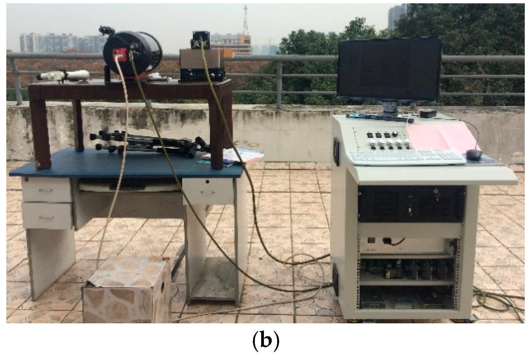
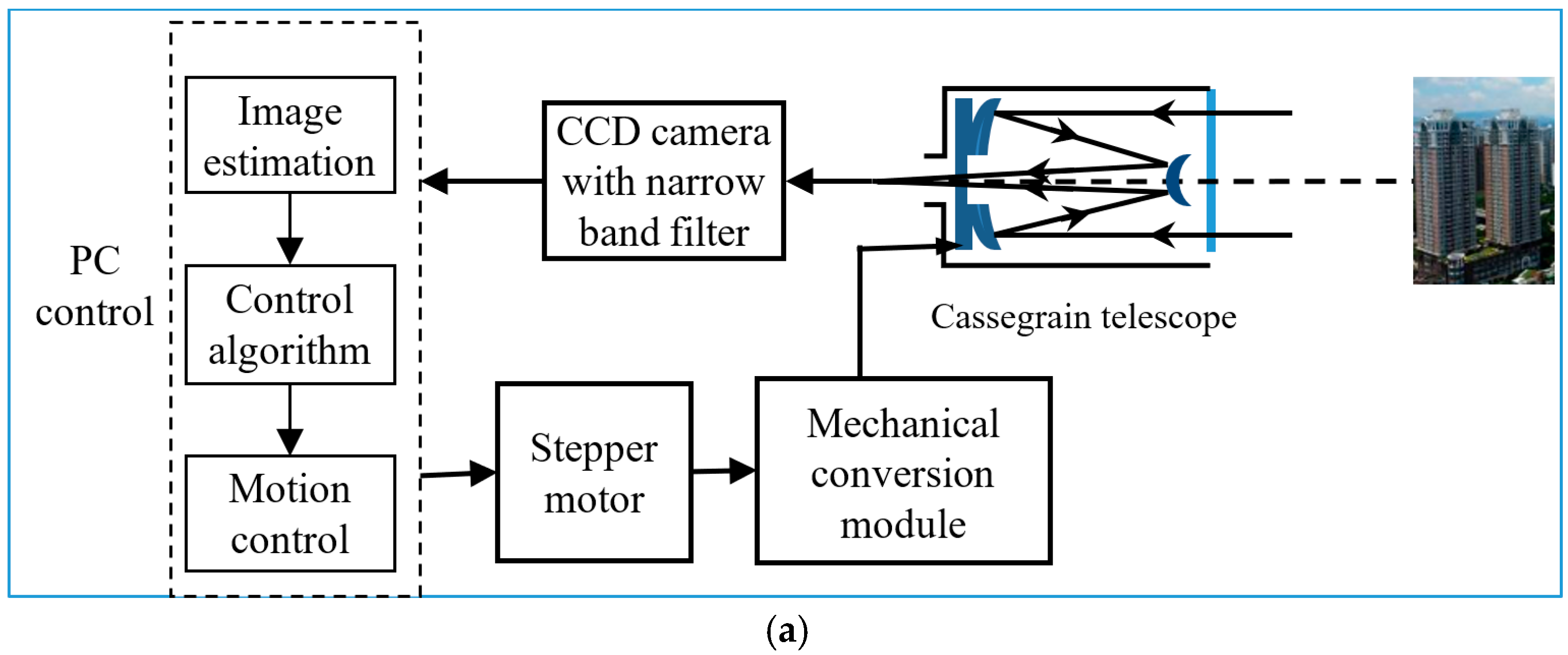
Applying the auto-focus principle above, the AFT of a Cassegrain telescope EOTS system was investigated, as shown in Figure 1. The EOTS system mainly consists of five parts [21]: Cassegrain telescope, CCD camera, PC control module, stepper motor, and mechanical conversion module. In the experiment, a Cassegrain telescope composed of a fold back mirror structure with two primary and secondary parabolic reflectors was used to collect the information of detected objects. To enhance the imaging quality, a Schmidt corrector was mounted in front of the telescope; there was also a CCD [22] camera with a narrow band filter to detect the image and to send the filtered results to the PC control module. In the control module, based on the image estimation, a stepper motor was used to adjust the position of the primary mirror of the telescope in the control device.

In Figure 1, the auto-focus process is given as follows [23,24]: firstly, the CCD camera captures information of tracked objects through the telescope and sends the image to the PC control program. Next, the PC control program performs an estimation of the CCD image and sends commands to rotate the stepper motor in a clockwise or counter-clockwise direction. Then, a mechanical conversion module turns the rotation force into a driver that adjusts the position of the primary mirror in the telescope forward or backward, and subsequently changes the imaging position. The above processes are repeated until the CCD camera is on the image plane of the telescope so that a clear image is obtained, making this auto-focus process a closed-loop system.

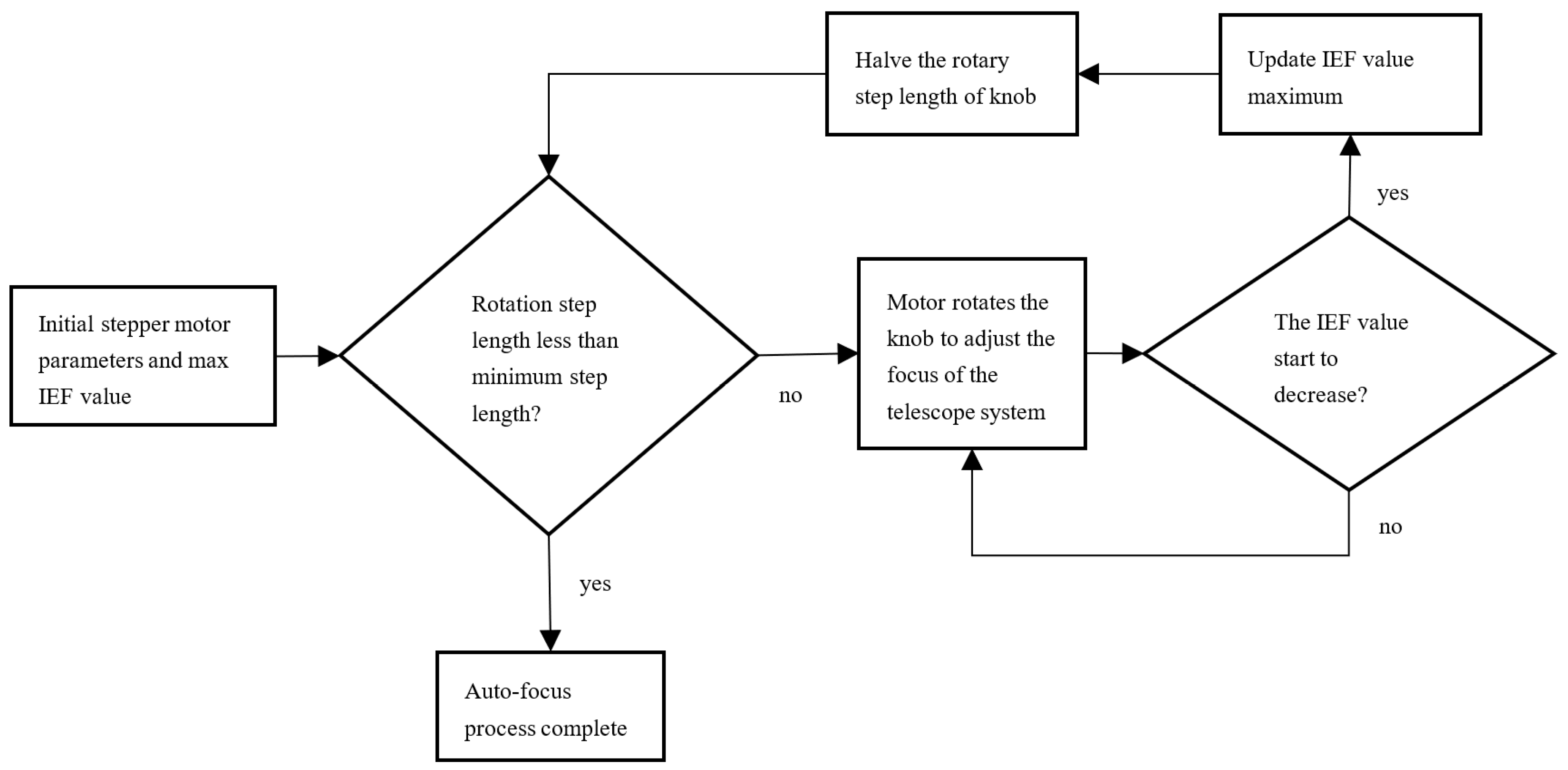
The focus search algorithm determines the concrete focus process of the system. In the experiment, the hill-climbing search method was used to achieve a better focusing effect. The specific steps are shown in Figure 2. First, we initialize the starting position of the motor knob and set a large initial rotation step length, recording the initial IEF value as the maximum value. The stepper motor rotates the knob at the current step length to adjust the focal length of the system and constantly calculates the IEF value. When the IEF value starts to decrease, it means that the best focusing position has been missed, and the knob is then rotated one step backward. Then, the current step length size is halved and the above search process is repeated until the search is completed with the minimum step size (accuracy) of the stepper motor. Then, the auto-focus process can be considered as finished.

3. Comparison of Image Estimation Functions

Different scenes, as captured by the EOTS, are shown in Figure 3. In the experiment, the CCD was first adjusted to find the correct focus position for each case. Then, the stepper motor was controlled to give a fixed clockwise and counterclockwise rotation angle, leading to a fixed moving distance of the primary mirror. When the CCD camera was in front of, located at, and behind the image plane, 17 pictures were obtained continuously for each of the scenarios shown in Figure 3.

In our auto-focus process, the sharpness of the image captured by the CCD camera should be estimated firstly. Currently, the most commonly used image intelligibility estimation functions (IEF) are mainly performed in the spatial and frequency domains. Spatial domain IEFs include the Tenengrad function [25], Brenner function [26], variance function, and Laplace function [27], while the frequency domain IEFs mainly include the wavelet function and statistical gray level entropy functions [28]. Compared to blurred images, clear images have more detailed information in the spatial domain, and the gray scale gradients of adjacent pixels are relatively large. A suitable image function supports us in determining whether the image is focused or not, which is a pivotal step in the auto-focus process [29]. In order to provide an accurate comparison of the focusing sensitivity, the estimation function was normalized by the ratio of the peak deviation to the maximum value of the function and defined as

$$S=\frac{E_{max}-E_{min}}{E_{max}}$$

(1)

where S is the normalized function value, and E_max and E_min are the maximum and minimum values, respectively, of the original estimation function.

(1) Tenengrad Function

The Tenengrad function takes the sum of the squares of image gradients as the evaluation index, and the gradients include horizontal and vertical directions [30]. The Sobel operator and image convolution are used to realize the function, which is written as

$$E={\displaystyle \sum _x{\displaystyle \sum _y{[S(x,y)]}^2}}$$

(2)

where $S(x,y)$ is the convolution of the pixel value of point $(x,y)$ and the Sobel operator, and it can be calculated as

$$S(x,y)=\sqrt{G_x^2(x,y)+G_y^2(x,y)}$$

(3)

where Gx and Gy are the horizontal and vertical gradients extracted by the Sobel operator, respectively.

Table 1. The change of the Tenengrad function during focusing in different scenes.

Scene a	Scene b	Scene c	Scene d	Scene e	Scene f	Scene g	Scene h
0.5373	0.8120	0.7846	0.8407	0.8125	0.7576	0.7773	0.9630
0.6268	0.8524	0.8345	0.9189	0.8889	0.8033	0.8430	0.9673
0.9906	0.9780	0.9328	0.9735	0.9748	0.9048	0.9726	0.9782
1.0000	1.0000	1.0000	1.0000	1.0000	1.0000	1.0000	1.0000
0.7947	0.9658	0.8437	0.7972	0.9530	0.8274	0.9637	0.9871
0.6390	0.9234	0.7534	0.7091	0.8995	0.7147	0.8439	0.9637
0.5564	0.8470	0.6928	0.6522	0.8022	0.6538	0.7638	0.9528

lists the Tenengrad function evaluation values of the focus position and the position of the front and back three steps in eight scenes. The fourth row of data presents the focus position function values.

(2) Brenner Function

The traditional Brenner function can extract the gradient information by calculating the gray difference between two adjacent pixels. It is the simplest method of gradient image evaluation. It can be expressed as

$$E={\displaystyle \sum _x{\displaystyle \sum _y{[f(x+2,y)-f(x,y)]}^2}}.$$

(4)

In order to ensure the focal length of the EOTS, the field-of-view angle is very small, so even if the distance is several kilometers, the field of view of telescope observation is also very small, as only a small part of the object is the target. If this part of the object does not have obvious texture, the Brenner function only contains the gradient information in the transverse direction and does not provide statistics on the longitudinal gradient; this may cause that part of the edge information to be lost, which affects the focusing accuracy. Therefore, based on the Brenner function, the longitudinal gray gradient is added, and the calculation method is as follows [31]:

$$E={\displaystyle \sum _x{\displaystyle \sum _y({(f(x+2,y)-f(x,y))}^2+{(f(x,y+2)-f(x,y))}^2)}}.$$

(5)

Table 2. The change of the Brenner function during focusing in different scenes.

Scene a	Scene b	Scene c	Scene d	Scene e	Scene f	Scene g	Scene h
0.7430	0.9486	0.8742	0.8537	0.8926	0.9478	0.8835	0.9784
0.7636	0.9522	0.8851	0.9236	0.9234	0.9585	0.9127	0.9922
0.9685	0.9987	0.9295	0.9412	0.9537	0.9635	0.9648	0.9993
1.0000	1.0000	1.0000	1.0000	1.0000	1.0000	1.0000	1.0000
0.8469	0.9657	0.9091	0.9318	0.9618	0.9697	0.9730	0.9458
0.7962	0.9274	0.8611	0.8662	0.9062	0.9256	0.9123	0.9176
0.7406	0.8486	0.8428	0.7475	0.8275	0.8925	0.8403	0.8992

lists the Brenner function evaluation values of the focus position and the position of the front and back three steps in eight scenes. The fourth row of data presents the focus position function value.

(3) Variance

A clear image has a larger gray scale difference than a fuzzy image, which shows that the variance of the image is larger, so the variance function is usually used to represent the gradient information of the image. The variance function can be expressed as

$$E={\displaystyle \sum _x{\displaystyle \sum _y{[f(x,y)-u]}^2}}$$

(6)

where u represents the average gray level of the image, and takes the following form:

$$u=\frac{1}{MN}{\displaystyle \sum _x{\displaystyle \sum _{y}f(x,y)}}$$

(7)

where M and N are the image dimensions.

Table 3. The change of the variance function during focusing in different scenes.

Scene a	Scene b	Scene c	Scene d	Scene e	Scene f	Scene g	Scene h
0.8253	0.9182	0.8879	0.8534	0.8842	0.8842	0.8994	0.9681
0.8525	0.9342	0.9038	0.8842	0.9234	0.9055	0.9146	0.9842
0.9715	0.9832	0.9437	0.9714	0.9389	0.9593	0.9762	0.9973
1.0000	1.0000	1.0000	1.0000	1.0000	1.0000	1.0000	1.0000
0.9194	0.9741	0.9194	0.9342	0.9734	0.9294	0l9537	0.9748
0.8621	0.9325	0.8856	0.8792	0.863	0.8913	0.8774	0.9695
0.8423	0.8832	0.8723	0.8344	0.7841	0.8725	0.8122	0.9599

lists the variance function evaluation values of the focus position and the position of the front and back three steps in eight scenes. The fourth row of data presents the focus position function value.

(4) Laplace Function

The Laplace function is also a commonly used method to evaluate the gray difference in an image, including 4-domain and 8-domain Laplace templates. In order to maximize the gradient information of the image, 8-domain Laplace templates were used in the experiment and can be obtained as

$$E={\displaystyle \sum _x{\displaystyle \sum _y\left|\begin{array}{l}8f(x,y)-f(x-1,y-1)-f(x-1,y)\\ -f(x-1,y+1)-f(x,y-1)-f(x,y+1)\\ -f(x+1,y-1)-f(x+1,y)-f(x+1,y+1)\end{array}\right|}}.$$

(8)

Table 4. The change of the Laplace function during focusing in different scenes.

Scene a	Scene b	Scene c	Scene d	Scene e	Scene f	Scene g	Scene h
0.6642	0.9658	0.8443	0.7425	0.8892	0.8442	0.7559	0.9536
0.7354	0.9904	0.8651	0.7935	0.9117	0.8639	0.8248	0.9810
0.8543	1.0000	0.9318	0.9051	0.9610	0.9317	0.9146	0.9983
1.0000	0.9835	1.0000	1.0000	1.0000	1.0000	1.0000	1.0000
0.8523	0.9734	0.9073	0.8754	0.9626	0.9252	0.9236	0.9881
0.7332	0.9256	0.8426	0.7640	0.9173	0.8631	0.8648	0.9689
0.6942	0.9052	0.7932	0.7223	0.8246	0.7980	0.7226	0.9677

lists the Laplace function evaluation values of the focus position and the position of the front and back three steps in eight scenes. The fourth row of data presents the focus position function value.

(5) Entropy

The entropy function is based on the premise that the clearer the image is, the more information it contains—that is, the greater the entropy of the image—so the entropy function can also be used to reflect the clarity of the image. The entropy function is calculated by

$$E={\displaystyle \sum _x{\displaystyle \sum _y-f(x,y)\ln [f(x,y)]}}.$$

(9)

Table 5. The change of the entropy function during focusing in different scenes.

Scene a	Scene b	Scene c	Scene d	Scene e	Scene f	Scene g	Scene h
0.9722	0.9810	0.9174	0.9485	0.9557	0.9347	0.9527	0.9510
0.9881	0.9583	0.9246	0.9477	0.9485	0.9638	0.9736	0.9659
0.9901	0.9831	0.9050	0.9531	0.9602	0.9750	09801	0.9483
1.0000	0.9677	1.0000	0.9335	0.9647	1.0000	1.0000	0.9631
0.9598	0.9432	0.9378	0.9546	1.0000	0.9345	0.9734	0.9577
0.9626	0.9259	0.8893	0.9539	0.9520	0.9130	0.9526	0.9731
0.9762	0.9376	0.8734	0.9665	0.9663	0.8773	0.9257	0.9677

lists the entropy function evaluation values of the focus position and the position of the front and back three steps in eight scenes. The fourth row of data presents the focus position function value.

For all these scenes, the sharpness estimations by the aforementioned IEFs of the captured image curves were calculated and are shown in Figure 4. In order to analyze the performance of each IEF, a whole-area focusing window was adopted, i.e., the whole picture was involved in the image estimation. For each subfigure in Figure 4, the abscissa and the ordinate are the picture sequence (where the ninth is the correct focus of the picture) and the normalized estimation function value, respectively.

In Figure 4a–h, the entropy function has multiple peaks, indicating the presence of instability. In Figure 4h, the Brenner function and the Laplace function also have multiple extrema which are not applicable. In terms of the unimodal property found in the corresponding eight scenarios, the Tenengrad and the variance IEFs are relatively stable. In addition, the normalized Tenengrad IEF value drops faster on both sides of the peak, indicating that the Tenengrad IEF has higher sensitivity than the variance one. In order to quantify the focusing effect of different IEFs, the efficiency factors was defined as

$$\mathrm{Ef}=\frac{E_{max}-E_{min}}{E_{max}+E_{min}}$$

(10)

where E_max and E_min represent the maximum and minimum values of the IEF, respectively. The higher the value of Ef is, the better the focusing effect is.

Table 6. Ef values of different IEFs in the eight scenarios.

	Tenengrad	Brenner	Variance	Laplace	Entropy
Scene a	0.371	0.156	0.131	0.250	0.027
Scene b	0.212	0.204	0.183	0.136	0.050
Scene c	0.273	0.104	0.111	0.156	0.049
Scene d	0.326	0.211	0.161	0.244	0.035
Scene e	0.289	0.215	0.214	0.240	0.080
Scene f	0.333	0.112	0.139	0.241	0.085
Scene g	0.321	0.186	0.183	0.293	0.063
Scene h	0.083	0.092	0.058	0.061	0.032

lists the Ef values of the different IEFs in the eight scenarios.

Based on the analysis above, the Tenengrad IEF shows its applicability in reflecting the focusing process in a variety of scenarios, and it can be used as an effective and stable estimation algorithm in the auto-focusing process of a telescope system. It was also found that all IEFs are also related to the properties of the scenarios themselves, and the sparser the scenarios (Figure 3h), the smoother the change in the IEF value.

4. An Improved Focusing Window Selection Method

In Section 3, we applied different IEFs to a whole-picture focusing window which contained lots of information. For telescope systems, it will take a long time to calculate the IEF values during digital image processing, resulting in the loss of the high-frequency part of the distinct edge and poor real-time performance of the system [32]. Further, in Scene h of Figure 3, because the image is sparse, all IEF values show smooth features, which will affect the accuracy of auto-focusing. In order to speed up the process and increase the accuracy of auto-focusing, a dynamic adaptive focusing window selection (DAFWS) method is presented.

In the DAFWS, the number of pixels is greatly reduced during sharpness estimation, and the time consumed by the calculation can be significantly shortened [33]. In the meantime, the application of a focusing window will also improve the quality, accuracy, and sensitivity of image estimation [34]. The traditional methods of sampling focusing windows [35,36], such as center window, multiple spots window, and inverted T window, only sample the pixels in the selected window uniformly, and information outside the window is completely lost. Besides, for these traditional approaches, the position of the target in the image must be determined before applying the auto-focus process, which will lead to an additional cost of calculation time [37]. Another drawback of these conventional methods is that the sharpness scores significantly depend on whether the target is in the selected focus window. Once the actual imaging target is not in the window or in the central position of the selected window, there will be a greater discrepancy between the IEF value and the actual situation.

In order to resolve this inadequacy, an efficient and accurate method is proposed. Firstly, instead of sampling inside a certain window, the whole image is sampled evenly, and the whole gray distribution feature of the image is retained. There is no need to locate the target in advance. Second, rather than setting the focus window before starting the auto-focus process, an adaptive method is applied to provide a dynamic focusing window. The pixels are divided into two categories: ROI (region of interest) pixels and background pixels. Experiments determined that the IEF values of the ROI pixels change greatly compared to the ones of the background pixels during the focusing process. Therefore, the ROI region can be selected out of the background region and extracted as the focus window. For example, the texture and boundary on the railing of Figure 3h have a greater impact on the estimation function, and they are the ROI. The sky part, belonging to the background region, is of no concern during the focusing process. The specific process of this even sampling–DAFW (ES-DAFW) method is given as follows.

An M × N image is divided into several m × n sub-blocks. Then, the IEF value of each sub-block can be given by the following formula:

$$E={\displaystyle \sum _{x=0}^{m-1}{\displaystyle \sum _{y=0}^{n-1}Tenengrad(x,y)}}$$

(11)

where (x, y) is the pixel coordinate in the sub-block, and E represents the Tenengrad IEF value of the image sub-block. The IEF value of each sub-block is recalculated as E′ after each rotation of the stepper motor. Then, the IEF value of each sub-block is normalized as

$$\mathsf{\Delta }=\frac{\left|E^{\prime }-E\right|}{E^{\prime }}$$

(12)

The threshold is set to u, then the sub-blocks with normalized IEF value larger than u (i.e., $\mathsf{\Delta }>u$) are ROI sub-blocks, while the remaining ones are considered as background blocks. For example, in Figure 5, a blurred picture with severe defocus of the scene in Figure 3h is divided into 8 × 8 blocks. Then, we used the Tenengrad IEF to calculate the normalized value of all sub-blocks in the auto-focus process, as shown in Figure 3h, and we chose five ROI sub-blocks with the largest change in the Δ value, as shown in black boxes in Figure 5.

To verify the effectiveness of the improved dynamic focusing window, for each of the images in Figure 3, we calculated the normalized values of the Tenengrad IEF for three focus window algorithms: whole-image focus window, traditional center window, and dynamic focus window. Figure 6a–h gives a comparison of the calculated results from the three methods.

Table 7. The average slopes of the three window selection methods around the focus position in different scenes.

	WIF	TCFW	ES-DAFW
Scene a	0.183	0.13	0.316
Scene b	0.071	0.075	0.161
Scene c	0.103	0.054	0.129
Scene d	0.093	0.05	0.174
Scene e	0.053	0.055	0.146
Scene f	0.120	0.035	0.155
Scene g	0.071	0.075	0.101
Scene h	0.018	0.012	0.047

shows the average slope of the IEF values around the peak value (positive focus position) under different window selection methods in the eight scenes. The larger the average slope, the more significant the change in the IEF value, which is helpful to improve the accuracy of the auto-focusing. From Figure 6 and Table 6, the curves of the whole-image focus window agree with the traditional center window very well for all scenarios, while the ES-DAFW method has sharper peaks than the other two methods. Especially in Figure 6h and Table 1, for Scene h, the improved performance of the ES-DAFW comes to a significant level when dealing with relatively sparse images like Figure 3h. In Figure 6h, the curves of the ES-DAFW method are much sharper than those calculated by the whole-image focus window and traditional center window methods, indicating a great improvement of the sensitivity of the IEF on both sides of the peak and, thereby, a fast auto-focus speed. We believe that in a telescope system with sparse imaging substance, this ES-DAFW would achieve a more accurate and much faster auto-focus process.

In order to compare the efficiency of different window selection methods in the auto-focusing process of the telescope EOTS system, we used whole-image focus (WIF), traditional center focus windows (TCFW), and ES-DAFW to test the auto-focus of the system ten times on the eight scenes in Figure 3, and we recorded the average time required for the completion of the auto-focus process, as shown in

Table 8. The average times taken by different window selection methods to complete auto-focusing.

	WIF(s)	TCFW(s)	ES-DAFW(s)
Scene a	8.36	6.37	3.27
Scene b	7.94	6.58	3.54
Scene c	8.12	6.14	4.79
Scene d	6.37	5.24	3.71
Scene e	9.28	7.64	4.39
Scene f	7.83	7.14	4.03
Scene g	9.28	6.39	5.17
Scene h	12.41	10.75	6.32

. It can be seen that in the case of sparse scenes, as shown in Table 8, the traditional method takes longer to complete the auto-focus process. ES-DAFW can take less time to complete the auto-focus process in all scenes, including sparse scenes, because it only uses the blocks in the image whose IEF value changes greatly. This will significantly improve the auto-focus efficiency of the telescope EOTS system.

5. Conclusions

Accurate and rapid auto-focus methods based on image quality assessment were studied in this paper, and the accuracy and sensitivity of various IEFs on different scenes were compared. Further, in order to improve the performance of IEFs, the ES-DAFW method was proposed based on the existing focus window selection method and was compared with the traditional method. Based on the above experiments and analysis, we summarize as follows:

(1)

In many image scenes collected by telescope, the Tenengrad function has high sensitivity (slope) near the peak value, which can better reflect the defocusing process of telescope system imaging. It is thus suitable as the estimation function of a telescope system;

(2)

From the experimental results of different focusing window methods, it can be seen that the ES-DAFW method can provide higher sensitivity and more accurate results for the auto-focus process, especially for a sparse image, when compared with the whole-image focusing window and the traditional center focusing window selection methods. At the same time, it has the advantages of simple calculation and can obviously shorten the time required for auto-focusing. These results promise significant applications to auto-focusing in other telescopes with EOTSs.