Study on the Shifting Quality of the CVT Tractor under Hydraulic System Failure

Abstract

The failure of a hydraulic system will affect the shifting quality and driving safety of a CVT tractor. In order to reveal the response of the tractor under different hydraulic system failures without destroying the transmission, the following methods are proposed in this paper: firstly, building the simulation model of CVT; secondly, building a test bench to test and verify the transmission model to ensure that the simulation model can accurately predict the response of CVT under different clutch oil pressures; thirdly, obtaining the fault oil pressure data without starting the engine and taking the data of fault oil pressure as the input variable of the simulation model; finally, obtaining the response of the CVT tractor under different hydraulic system failures by simulation. It is found that the damage of the seal ring inside the rotary joint has little effect on shifting quality; oil way block can lead to greater shift impact; when seal ring damage and oil way block occur together, the clutch cannot reach the minimum working pressure; clutch piston jamming and oil leak can cause power interruption of the tractor. The results show that it is feasible to study the response of CVT in fault mode by simulation.

1. Introduction

A tractor’s working conditions are complex, and it often needs more working gears. For example, Foton Lovol’s P2654-N tractor and Changfa’s CFK2204 tractor have 40 forward gears and 40 reverse gears. Excessive working gears make the transmission structure complex; therefore, CVT (continuously variable transmission) becomes an ideal tractor transmission system [1]. Since Fendt [2] first equipped hydrostatic power split CVT in tractors in 1996, ZF, Claas, John Deere, and other companies have successively developed their own tractor CVTs, such as the S-Matic transmission produced by ZF, the Eccom transmission and Traxion transmission produced by Claas, the AutoPowr transmission produced by John Deere, etc. [3]. However, different from the design of Fendt, these CVTs generally use multi-range speed control technology, which can effectively reduce the energy loss of the hydraulic system and improve the fuel economy of the tractor [4,5], but the premise is to solve the problem of power shift. The principle of power shift [6,7,8] is to ensure the continuous power transmission during the shift by the sliding friction of the wet clutch, which is very important for tractors that often work in heavy load conditions. The hydrostatic power split CVT is a complex mechanic-electronic-hydraulic integrated system, which requires high robustness and reliability for each subsystem [9,10,11]. Once the hydraulic system that controls the clutches fails, it may affect the driving comfort and even endanger the driving safety during the shift [12,13]. In recent years, some enterprises and universities in China have successfully developed their own tractor CVTs [14,15,16], but industrialization has never been realized, one of the important reasons being the high failure rate. The research of fault problem needs test data as support. However, in order to obtain the test data when the fault occurs, the usual method is to destroy the research object. For example, Park et al. [17] used wire cut electric discharge machining to generate the spall and the crack on the gear surface for transmission fault simulation. Huang et al. [18] did a similar work: two types of ringing defect, including outer race and rolling element fault, were manually scratched in the research. Compared with the ordinary transmission, Chang et al. [19] studied the fault diagnosis of the planetary gearbox, and eight bearing and gear faults were manually manufactured. However, the cost of the hydrostatic power split CVT is very high. Damage to the hydraulic system for research purposes can lead to unpredictable consequences, such as permanent damage to the clutch or transmission, which is not acceptable in terms of cost. Therefore, there is little research on the fault problem of the hydrostatic power split CVT, especially its shifting process. In order to evaluate the impact of hydraulic system failure on the shifting quality and driving safety without damaging the tractor CVT, the following method is proposed in this paper: first, the oil pressure data of the transmission clutch under different hydraulic system faults are obtained without starting the engine, and then, the response of the CVT tractor to the fault oil pressure is obtained by computer simulation.

2. Principle of Hydrostatic Power Split CVT

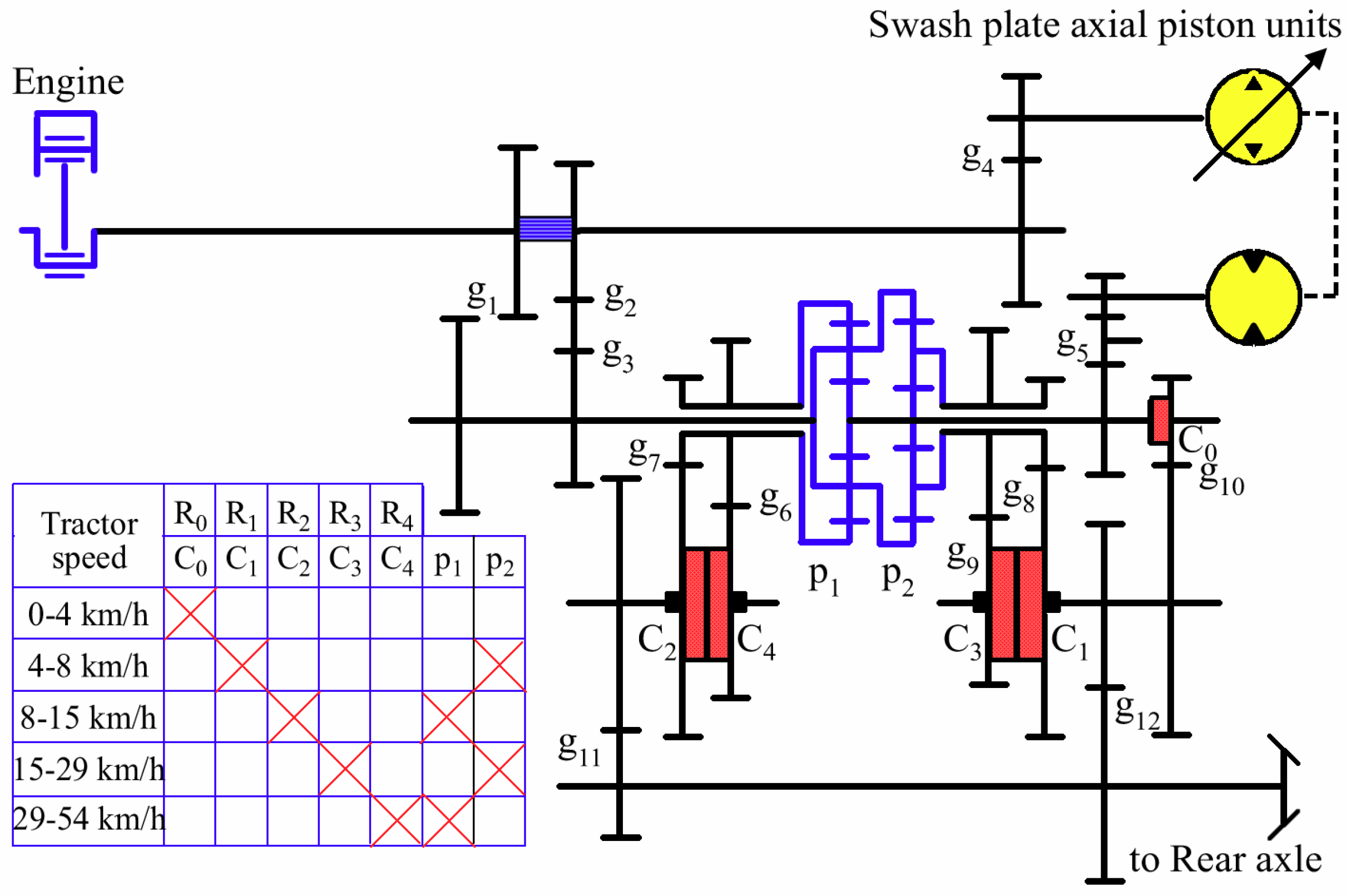
2.1. Analysis of the Transmission System

The transmission system of the hydrostatic power split CVT is shown in Figure 1. The rated engine power of the transmission was 132.5 kW. Range R₀ was used to start up with 100% hydraulic power, and ranges R₁–R₄ were used to keep the hydrostatic power level low, while only one clutch of each range was in the working state. The planetary gear set p₁ and p₂ formed a four shaft compound planetary gear for power merging. The planetary gear set p₁ worked in ranges R₂ and R₄, while planetary gear set p₂ worked in ranges R₁ and R₃. The transmission could be started by hydrostatic transmission, and the tractor speed could be adjusted continuously in the range of 0–50 km/h.

When the wet clutch C₀ was engaged, the engine power was transmitted to the output shaft through the gear pair g₄, the swash plate axial piston units, the gear pair g₅, the clutch C₀, and the gear pair g₁₀ and g₁₂. When the clutch C₁/C₃ was engaged, the engine power was divided into two parts: one part of the engine power flowed into the sun gear of the planetary gear set p₂ through the gear pair g₄, the swash plate axial piston units, and the gear pair g₅, and the other part of the engine power flowed into the ring gear of the planetary gear set p₂ through the gear pair g₂ and g₃. The two parts of the engine power were merged in the carrier of the planetary gear set p₂ and then transmitted to the output shaft through the gear pair g₈/g₉ and clutch C₁/C₃. When the clutch C₂/C₄ was engaged, the engine power was divided into two parts: one part of the engine power flowed into the sun gear of the planetary gear set p₁ through the gear pair g₄, the swash plate axial piston units, and the gear pair g₅, and the other part of the engine power flowed into the carrier of the planetary gear set p₁ through the gear pair g₂ and g₃. The two parts of the engine power were merged in the ring gear of the planetary gear set p₁ and then transmitted to the output shaft through the gear pair g₇/g₆ and clutch C₂/C₄.

The engagement states of clutches C₀–C₄ was controlled by the hydraulic control system, as shown in Figure 2. When the solenoid valve was energized, the hydraulic oil entered the clutch hydraulic cylinder and pushed the piston to engage the driving and driven friction plates; otherwise, when the solenoid valve was powered off, the hydraulic oil was connected with the oil tank, the piston reset under the action of the return spring, and the driving and driven friction plates of the clutch were separated. The working pressure and flow of each clutch were set by the relief valve and the speed control valve, respectively. A pressure sensor was installed on each working oil circuit, while a pressure sensor and a flow sensor were installed on the main oil circuit.

2.2. Basic Transmission Equations

Consider that the rotation speed of each planetary gear shaft meets the conditions [20]:

$$n_s+k{n}_r-\left(1+k\right)n_c=0$$

(1)

where $n_s$, $n_r$, and $n_c$ are the rotation speed of sun gear, ring gear, and carrier of the planetary gear set, respectively, r/min; $k$ is the standing ratio of planetary gear set, which is the ratio of sun gear and ring gear speed with a fixed planet carrier.

The speed relationship between pump shaft and motor shaft is as follows:

$$n_m=n_p\epsilon$$

(2)

where $n_m$ and $n_p$ are the rotation speeds of the fixed displacement motor (MF) and the variable displacement pump (PV), r/min, respectively; $\epsilon$ is the displacement ratio of the swash plate axial piston units.

It is easy to deduce that the transmission ratio of the CVT in each range is:

$$n_{R1}\left(\epsilon \right)=\frac{k_2{i}_4{i}_5-i_2{i}_3\epsilon }{\left(1+k_2\right)i_2{i}_3{i}_4{i}_5{i}_8{i}_{12}}{n}_e$$

(3)

$$n_{R2}\left(\epsilon \right)=\frac{\left(1+k_1\right)i_4{i}_5+i_2{i}_3\epsilon }{k_1{i}_2{i}_3{i}_4{i}_5{i}_7{i}_{11}}{n}_e$$

(4)

$$n_{R3}\left(\epsilon \right)=\frac{k_2{i}_4{i}_5-i_2{i}_3\epsilon }{\left(1+k_2\right)i_2{i}_3{i}_4{i}_5{i}_9{i}_{12}}{n}_e$$

(5)

$$n_{R4}\left(\epsilon \right)=\frac{\left(1+k_1\right)i_4{i}_5+i_2{i}_3\epsilon }{k_1{i}_2{i}_3{i}_4{i}_5{i}_6{i}_{11}}{n}_e$$

(6)

where $n_{Rx}$ is the output speed of the transmission in range R_x (x = 1, 2, 3, 4), which is a function of the displacement ratio $\epsilon$, r/min; $i_2$~$i_{12}$ are the transmission ratios of gear pairs g₂~g₁₂, respectively; $k_1$ and $k_2$ are the standing ratios of the planetary gear set p₁ and p₂, respectively; $n_e$ is the engine speed, r/min.

In order to achieve excellent acceleration performance, the speed regulation range of two adjacent ranges must meet the equal ratio condition:

$$\frac{n_{Rx}\left({\epsilon }^{*}\right)}{n_{Rx}\left(-{\epsilon }^{*}\right)}=\phi$$

(7)

where $\phi$ is the common ratio of each range; ${\epsilon }^{*}$ is the displacement ratio corresponding to the maximum tractor speed in range R_x. ${\epsilon }^{*}$ = −1 if $x$ = 1 or $x$ = 3, and ${\epsilon }^{*}$ = 1 if $x$ = 2 or $x$ = 4.

According to Equations (3)–(7), the following relationship can be obtained:

$$\frac{i_4{i}_5}{i_2{i}_3}=\frac{\phi +1}{k_2\left(\phi -1\right)}$$

(8)

$$\frac{i_4{i}_5}{i_2{i}_3}=\frac{\phi +1}{\left(1+k_1\right)\left(\phi -1\right)}$$

(9)

Comparing Equations (8) and (9), it is easy to get:

$$1+k_1=k_2$$

(10)

In addition, in order to make each range connect at the maximum pump displacement, the connection conditions shall also be met:

$$n_{R1}\left(-1\right)=n_{R2}\left(-1\right)$$

(11)

$$n_{R2}\left(1\right)=n_{R3}\left(1\right)$$

(12)

$$n_{R3}\left(-1\right)=n_{R4}\left(-1\right)$$

(13)

By substituting Equations (3)–(6) into Equations (11)–(13), the following relationship can be obtained:

$$\frac{i_8{i}_{12}}{i_7{i}_{11}}=\frac{\phi \left(k_2-1\right)}{1+k_2}$$

(14)

$$\frac{i_7{i}_{11}}{i_9{i}_{12}}=\frac{\phi \left(k_2+1\right)}{k_2-1}$$

(15)

$$\frac{i_9{i}_{12}}{i_6{i}_{11}}=\frac{\phi \left(k_2-1\right)}{1+k_2}$$

(16)

In conclusion, the output speed of the CVT calculated by Equations (3)–(6) was reasonable only when Equation (10) and Equations (14)–(16) were satisfied. According to Equations (3)–(6), the relationship between the output speed of the transmission in each range and the displacement ratio of the swash plate axial piston units could be calculated. The actual output speed of the transmission could be obtained by testing at different engine speeds, ranges, and displacement ratios. The calculation results of the transmission output speed were consistent with the test results, as shown in Figure 3. It can be seen from the figure that the transmission had the same displacement ratio and the same output speed before and after the shift, so the shift process under ideal conditions should be relatively smooth.

3. Construction of the Shifting Dynamics Model

3.1. Model of Swash Plate Axial Piston Units

The swash plate axial piston units were composed of a variable displacement pump and constant displacement motor with the same rated displacement, which was the core speed regulating component of the CVT; its essence was the volume speed modulating loop. The relationship between the torque and the rotational speed of the pump shaft is as follows:

$$T_p=\frac{p_{AB}\epsilon V_p}{20\pi }$$

(17)

$$n_p=\frac{1000Q_{AB}}{\epsilon V_p}$$

(18)

where $p_{AB}$ is the pressure difference of the two hydraulic ports of the pump, bar; $Q_{AB}$ is the volume flow of the pump, L/min; $T_p$ is the torque of the pump shaft, N·m; $V_p$ is the rated displacement of the pump, cm³/r. In particular, Equations (17) and (18) can also be used to describe the motor when $\epsilon \equiv 1$.

3.2. Model of the Gear

The rotation speed and torque of the common gear meet the following relationship:

$$n_2=\frac{n_1}{i_{12}}$$

(19)

$$T_2=i_{12}{T}_1$$

(20)

where $i_{12}$ is the transmission ratio of the gear pair; $n_1$ and $n_2$ are the rotating speed of the driving gear and driven gear, r/min, respectively; $T_1$ and $T_2$ are the torque of the driving gear and driven gear, N·m, respectively.

The speed of each planetary gear shaft could be calculated by Equation (1), and the torque of each planetary gear shaft meets the following relationship [21]:

$$T_s:T_r:T_c=1:k:\left(1+k\right)$$

(21)

where $T_s$, $T_r$, and $T_c$ are the torque of the sun gear, ring gear, and carrier of the planetary gear set, respectively, N·m.

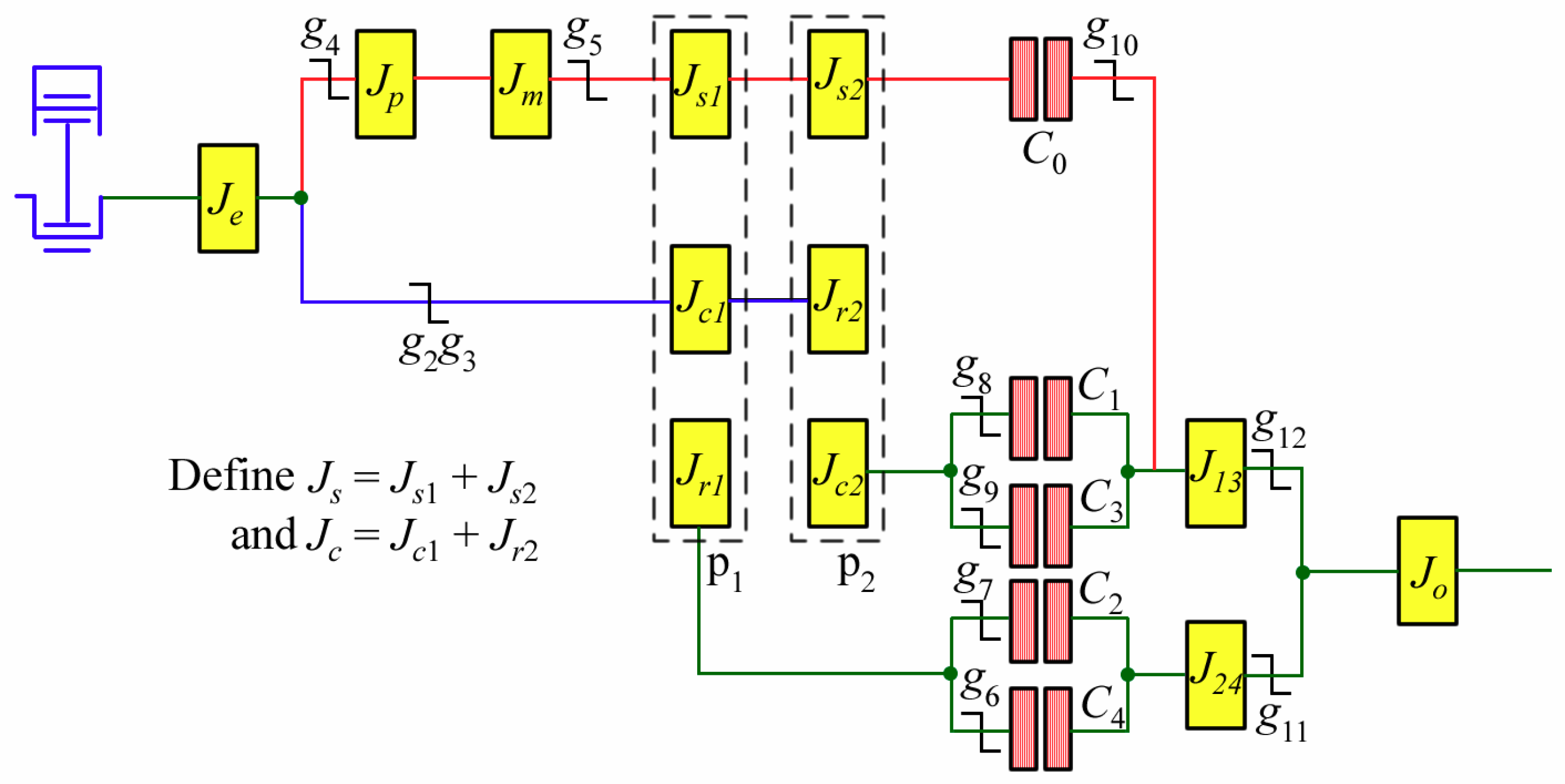
3.3. Model of the Shaft

In this study, the influence of the moment of inertia of the shaft on shifting quality cannot be ignored. Affected by the internal resistance and load of the transmission, the speed of the shaft will change during the shift [22,23]. Due to the existence of the moment of inertia, additional torque will be produced on the shaft:

$$T=T_0+J\alpha$$

(22)

where $T$ is the torque of the shaft, N·m; $T_0$ is the theoretical torque of the shaft, N·m; $J$ is the moment of inertia of the shaft, kg·m²; $\alpha$ is the angular acceleration of the shaft, rad/s².

Based on the foregoing considerations, the moment of inertia of each component must be calculated and equivalent to its adjacent shaft, as shown in Figure 4. Among them: $J_e$ is the moment of inertia of the engine shaft; $J_p$ and $J_m$ are the moments of inertia of the pump shaft and motor shaft, respectively; $J_{s1}$, $J_{r1}$, and $J_{c1}$ are the moments of inertia of the sun gear shaft, ring gear shaft, and carrier of the planetary gear set p₁, respectively; $J_{s2}$, $J_{r2}$, and $J_{c2}$ are the moments of inertia of the sun gear shaft, ring gear shaft, and carrier of the planetary gear set p₂, respectively; $J_{13}$ and $J_{24}$ are the moments of inertia of the two shafts installed with clutches C₁/C₃ and C₂/C₄, respectively; $J_o$ is the moment of inertia of the output shaft. Based on the software of SolidWorks, the virtual prototype model of each gear and shaft was built in this study. After defining the material properties (40Cr was used in most parts of the transmission), the moment of inertia of each gear and shaft could be directly calculated by SolidWorks. In particular, the moment of inertia of the clutch was provided by the manufacturer.

In addition, treating most shafts and gears (including the planetary gear set) as rigid bodies had no significant effect on the calculation results. However, the shaft of the speed and torque sensor used in the later test was an elastic shaft. Therefore, adding spring-damper models (see Figure 5) to the input and output shafts could avoid the violent oscillation of the simulation results which was inconsistent with the actual situation. The effect of stiffness and damping on the shaft torque could be expressed as follows:

$${\theta }_{kr}={\theta }_{ka}-{\theta }_{kb}$$

(23)

$${\omega }_{kr}={\omega }_{ka}-{\omega }_{kb}$$

(24)

$$T_k=k_a{\theta }_{ka}+b_a{\omega }_{kr}$$

(25)

where ${\theta }_{kr}$, ${\theta }_{ka}$, and ${\theta }_{kb}$ are the relative angular displacement, angular displacement of the driving port, and angular displacement of the driven port, respectively, rad; ${\omega }_{kr}$, ${\omega }_{ka}$, and ${\omega }_{kb}$ are the relative angular speed, angular speed of the driving port, and angular speed of the driven port, respectively, rad/s; $T_k$ is the total torque of the shaft; $k_a$ is the stiffness of the shaft, N·m/rad; $b_a$ is the damper rating of the shaft, N·m/(rad/s).

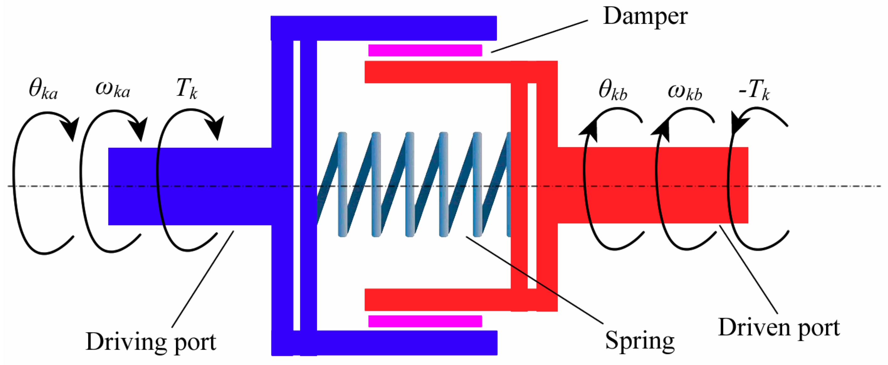
3.4. Model of the Clutch

The structure of the clutch is shown in Figure 6. When the oil pressure increased, the hydraulic oil pushed the piston to move and pressed the driving and driven friction plates, so that the driving and driven shafts were connected together; on the contrary, when the oil pressure decreased, the return spring pushed the piston to move in reverse and reset, thus interrupting the power transmission between the driving and driven shafts.

The sliding process between the driving and driven friction plates of the clutch directly affected the shifting quality of the transmission. As shown in Figure 7, the friction torque transmitted by the clutch depended on the normal force between the driving and driven friction plates [24,25]:

$$T_f=\frac{2\mu F_a{n}_f\left(r_o^3-r_i^3\right)}{3\left(r_o^2-r_i^2\right)}$$

(26)

where $T_f$ is the friction torque, N·m; $F_a$ is the normal force, N; $n_f$ is number of clutch contact faces; $r_o$ and $r_i$ are the outside and inside radius of the clutch plate, respectively, mm; $\mu$ is the actual speed dependent friction coefficient, which can be calculated as [26]:

$$\mu ={\mu }_0-\left({\mu }_0-{\mu }_s{\mathrm{M}}_1\right)tanh\left({\mathrm{M}}_2\left({\omega }_{ca}-{\omega }_{cb}\right)\right)+{\mathrm{M}}_3\left({\omega }_{ca}-{\omega }_{cb}\right)$$

(27)

where ${\omega }_{ca}$ and ${\omega }_{cb}$ are the speed of the driving shaft and driving shaft, rad/s; ${\mu }_0$ and ${\mu }_s$ are the sticking and slipping friction coefficients, respectively; ${\mathrm{M}}_1$–${\mathrm{M}}_3$ are constants related to friction materials.

For a wet clutch, the normal force $F_a$ is the resultant force of oil pressure and return spring force:

$$F_a=0.1\lambda pA-k_s\left(\Delta x+x_0\right)$$

(28)

where $\lambda \left(1<\lambda \le 1\right)$ is the frictional correction coefficient, and $\lambda =1$ only when the clutch piston stops moving; $p$ is the oil pressure, bar; $A$ is the effective area of the clutch piston, mm²; $k_s$ is the stiffness of the return spring, N/mm; $\Delta x$ and $x_0$ are the displacement increment and initial displacement of the return spring, respectively, mm.

3.5. Model of Tractor

The dynamic model of the CVT tractor transmission system under SimulationX [27,28] included the engine and rear axle, and the CVT is shown in Figure 8. In this model, the relationship between the driving speed of tractor and the output speed of transmission is:

$$v_t=0.377\times \frac{n_o{r}_d}{i_m{i}_s}$$

(29)

where $v_t$ is the driving speed of the tractor, km/h; $n_0$ is the output speed of the transmission, r/min; $r_d$ is the dynamic radius of the driving wheel, m; $i_m$ and $i_s$ are the transmission ratios of the main drive and the wheel side reducer, respectively.

In particular, the simulation of the model required externally given pressure $p$ and displacement $x$ in Equation (25). In this study, the clutch pressure and return spring displacement under different working conditions were obtained by bench test, and they were used as input variables of the tractor model.

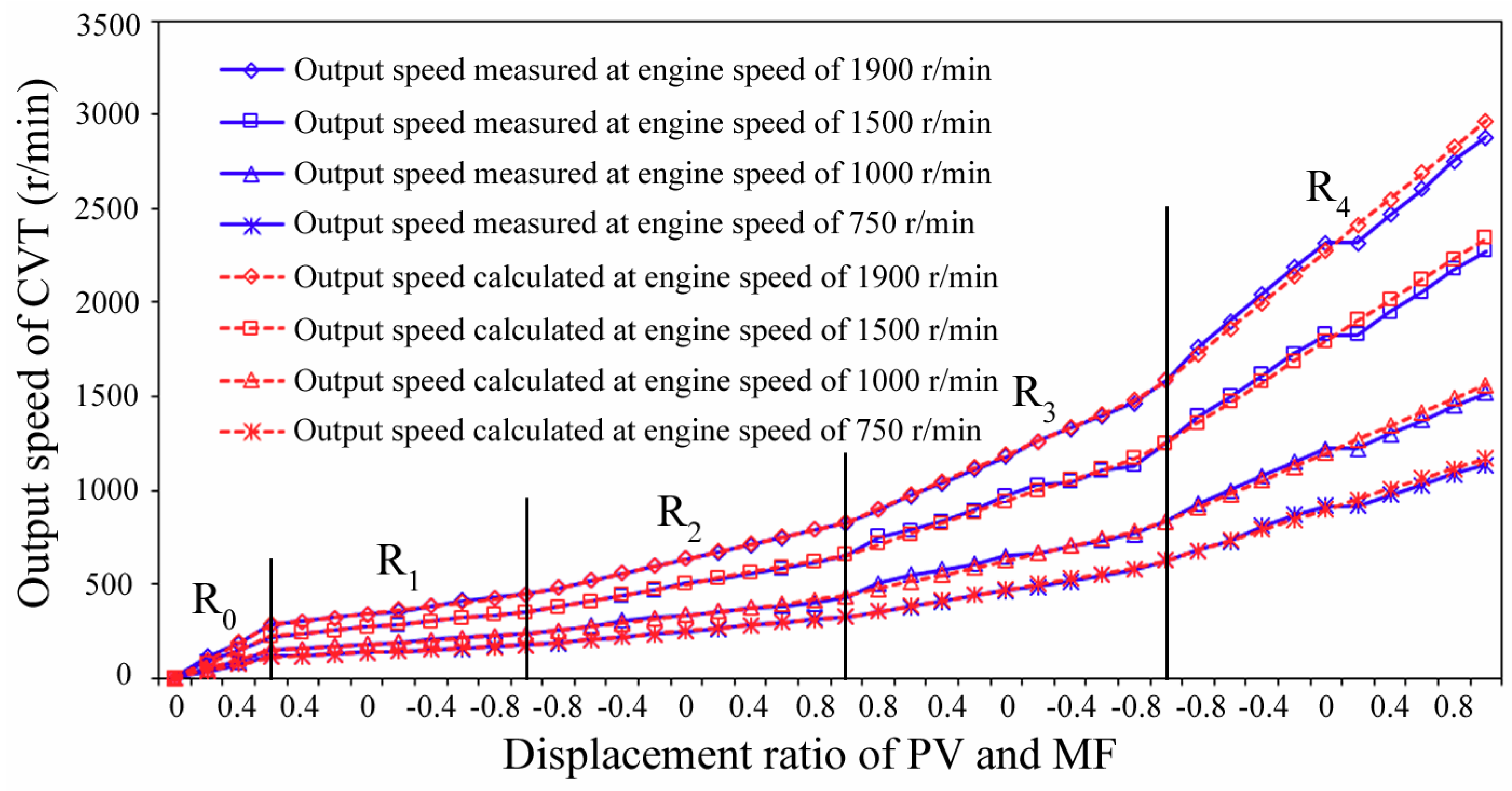
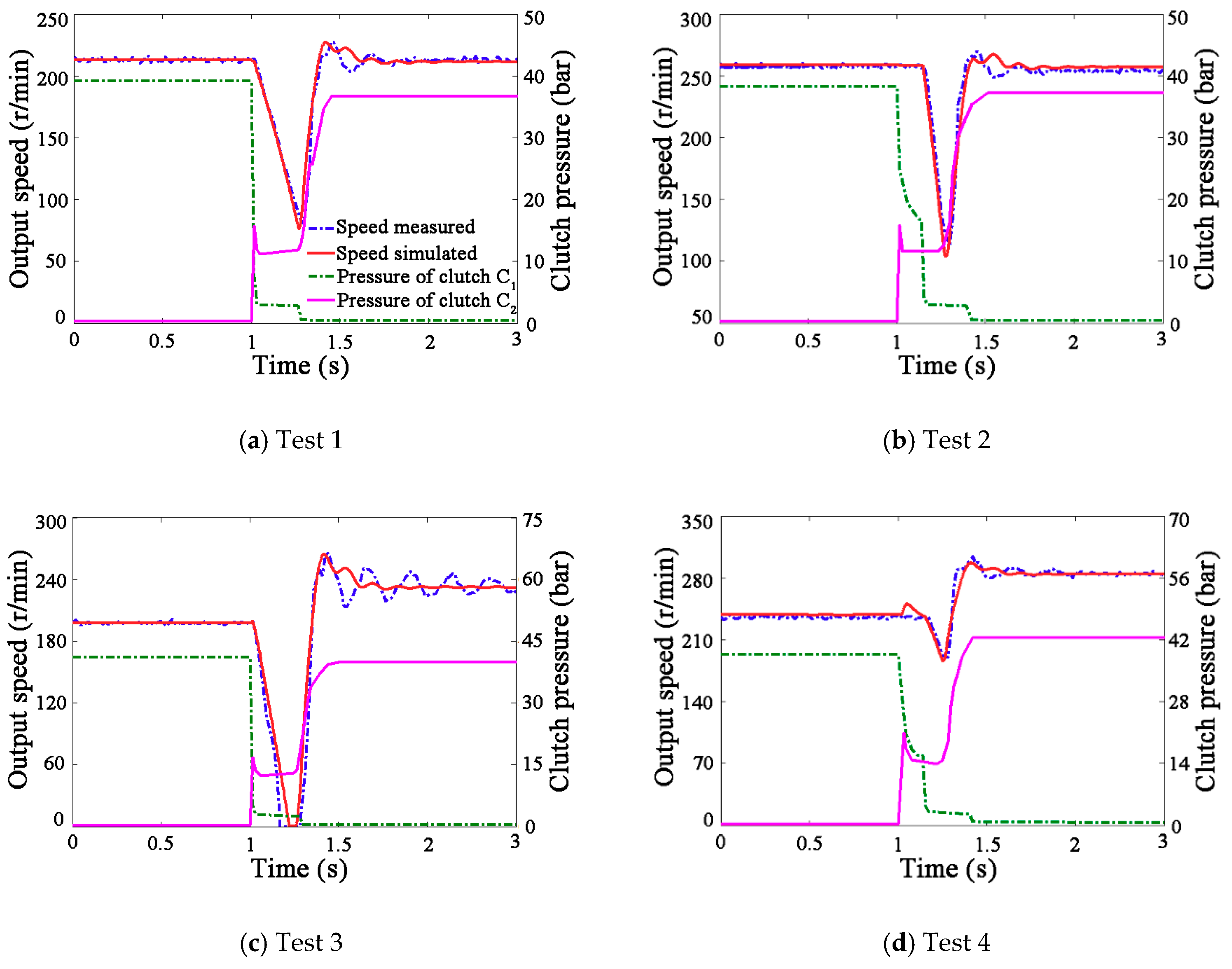
3.6. Test Verification

As shown in Figure 9, the test bench comprised a diesel engine (132.5 kW, 2200 r/min), two speed and torque sensors, a hydrostatic power split CVT, a magnetic powder brake, a clutch hydraulic control system, a TCU (transmission control unit), and a remote PC. The information of test equipment used in the test bench is shown in

Table 1. Test equipment.

No.	Name	Model	Parameter	Manufacturer
1	Diesel engine	WP6T180E21	Rated power: 132.5 kW Rated speed: 2200 r/min	Weichai Power
2	Hydrostatic power split CVT	-	Rated power: 132.5 kW Transmission ratio: 0.687–8.585	Self-development
3	Magnetic powder brake	CZ50	Braking torque: 500 N·m	Hangyu
4	Speed sensor	JC3A	Speed range: 0–3000 r/min	Xiangyi
5	Oil pressure sensor	NS-F	Pressure range: 0–100 bar	Tianmu

. Considering the following reasons, the test was only conducted between the range R₁ and the range R₂: the magnetic powder brake could only be used at low speed; the tractor worked in ranges R₁ and R₂ most of the time (the speed range of 4–12 km/h accounted for 68% of the total working time of the tractor [29]); the shifting process between ranges R₁ and R₂, R₂ and R₃, and R₃ and R₄ was the same.

After starting the engine, the speed regulation instruction was sent to TCU through the industrial computer. TCU energized the solenoid valve to engage the clutch C₁ and adjusted the displacement ratio of the variable displacement pump to “−1”. Then, the loading instruction was sent to the magnetic powder brake through the industrial computer and the special control circuit. When the load was stable, the engine speed was adjusted to the specified value through the electronic throttle. Finally, the shift instruction was sent to TCU through the industrial computer. TCU separated the clutch C₁ and engaged the clutch C₂. During the test, the computer read the sensor data of speed, torque, pressure, flow, and so on, in real time through the data acquisition card and recorded them in the disk file by software developed under LabVIEW at a frequency of 60 Hz. In order to ensure the reliability and repeatability of the test results, the engine needed to be preheated for more than 30 min before the start of the test, and each group of tests needed to be repeated many times until the three consecutive test results were basically the same.

The purpose of this study was not to predict the absolute true values of the shifting quality, but to reveal the influence law of hydraulic system failure on the shifting quality of the CVT tractor. Therefore, only the transmission model needed to be tested and verified. It was the core component of the CVT tractor. Four groups of shifting experiments were carried out under different limited flow, pump displacement, shift timing sequence, engine speed, and load, as shown in

Table 2. Test scheme of the power shift.

No.	Limited Flow (L/min)	Pump Displacement	Shift Timing Sequence (s)	Engine Speed (r/min)	Load (N·m)
1	4	1	0	900	150
2	4	1	0.15	1100	300
3	5	0.7	0	900	300
4	5	0.7	0.15	1100	150

. The measured and simulated results are shown in Figure 10a–d. According to the figure, the output shaft speed response of the simulation model to the same pressure input was consistent with the test results.

4. Fault Simulation and Analysis

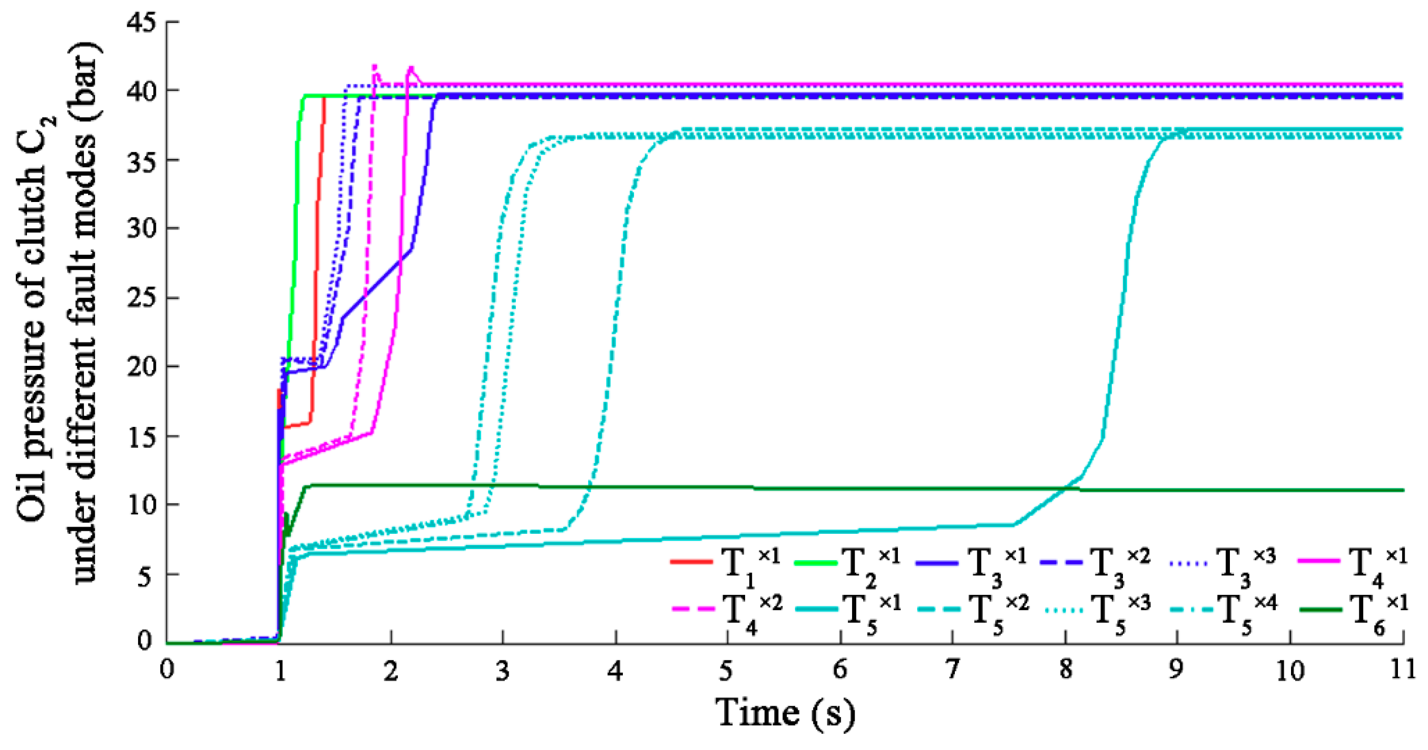
4.1. Fault Simulation

The clutch C₂ was taken as the research object of fault simulation. Six failure modes were created in the laboratory, including the normal mode T₁, piston jamming mode T₂, seal ring damaging mode T₃, oil way blocking mode T₄, oil leaking mode T₅, and T₃ × T₄ combined failure mode T₆.

For failure mode T₁, no change was needed to the hydraulic oil circuit; for failure mode T₂, the axial clearance between the clutch piston and the hydraulic cylinder could be filled with sandpaper before the solenoid valve was energized to make the piston unable to move; for failure mode T₃, the normal sealing ring at the rotary joint could be replaced by the damaged one; for failure mode T₄, the opening degree of speed control valve should be reduced; for failure mode T₅, the pipe joint should be loosened; for failure mode T₆, the damaged sealing ring and the smaller opening of the speed control valve could be used for simulation at the same time.

The oil pressure response of the engaged clutch C₂ under different failure modes is shown in Figure 11. It should be noted that the shape of the pressure curve in failure mode T₃–T₅ was related to the severity of the fault; therefore, different fault pressure curves were selected for calculation and analysis. Take failure mode T₃ as an example: pressure T₃^×1 corresponds to the serious damage of sealing ring, pressure T₃^×2 to the moderate damage of sealing ring, and pressure T₃^×3 to the slight damage of sealing ring.

Compared with the normal mode T₁, the failure mode T₂ had the fastest rise speed of oil pressure, but this was caused by the piston being stuck and unable to move. If the stuck position was close to the initial position of piston movement (the situation simulated in this study), the clutch could not be engaged all the time. On the contrary, if the stuck position was close to the end stop of piston movement, the clutch would always be in a half engaged state, and the clutch would be burnt out. Similar situations occurred in the laboratory, as shown in Figure 12. Although the failure modes T₃ and T₄ changed the shape of oil pressure curve to some extent, it could still achieve stable engagement pressure within 1.5 s. The failure mode T₅ not only caused the clutch to fail to reach the expected working pressure and reduced the load driving ability of the tractor, but it also delayed the engagement time of the clutch to a large extent, which may lead to power interruption. Although the failure mode T₆ was the test result of the combination of the failure modes T₃ and T₄, the shape of its oil pressure curve was completely different from the two failure modes, and its lower pressure could not drive the piston action.

4.2. Evaluation Indexes of Shifting Quality

During the shift process, the separation of the clutch C₁ would lead to the decrease of the tractor speed. The engagement of the clutch C₂ would lead to the increase of the tractor speed. Therefore, the speed of the tractor would fluctuate during the shift process, and the speed drop could be used as the first evaluation index of the shifting quality:

$$v_{drop}=v_o-v_{min}$$

(30)

where $v_{drop}$ is the speed drop of the tractor during the shift, r/min; $v_o$ and $v_{min}$ are the theoretical driving speed and the minimum driving speed of the tractor during the shift, respectively, r/min.

The research of Duncan [30] showed that the shifting quality that the human body can feel is closely related to the peak acceleration of the tractor. Therefore, this study took the maximum value of the acceleration during the shift as the second evaluation index of the shifting quality:

$$a_{peak}=\mathrm{Max}\left(\frac{d{v}_t}{dt}\right)$$

(31)

where $a_{peak}$ is the peak acceleration, m/s²; $t$ is the time, s.

In addition, the clutch would produce energy loss in the process of sliding; if the energy loss were too large, the service life of the clutch would be shortened. Therefore, the power and energy loss of the clutch during the shift were taken as the third and fourth evaluation indexes of the shifting quality, respectively:

$$P_{loss}=\mathrm{Max}\left(\frac{T_c\Delta \omega }{9550}\right)$$

(32)

$$W_{loss}=\underset{t_1}{\overset{t_2}{{\displaystyle \int }}}\frac{T_c\Delta \omega }{9550}dt$$

(33)

where $P_{loss}$ is the maximum power loss of the clutch during the shift, kW; $W_{loss}$ is the accumulated energy loss of the clutch during the shift, kJ; $t_1$ and $t_2$ are the starting time and ending time of the shift, respectively, s.

4.3. Simulation Conditions and Parameters

The simulation conditions were as follows: the tractor ran stably before the shift; the engine speed was 1500 r/min, the working load 20,000 N, and the tractor mass 10.5 t; the transmission shifted from the range R₁ to the range R₂.

The gear parameters of the transmission are shown in

Table 3. Transmission ratio of the gear pair used in the simulation.

i2	i3	i4	i5	i7	i8	i11	i12	k1	k2
0.97	1.48	0.68	1.96	3.52	2.77	0.82	1.09	2.56	3.56

. The equivalent moment of inertia of each shaft is shown in

Table 4. Equivalent moment of inertia used in the simulation (kg·m²).

Je	Jp	Jm	Js	Jc	Jr1	Jc2	J13	J24	J0
0.125	0.005	0.005	0.157	0.509	0.530	0.664	0.788	0.463	0.321

. The clutch parameters are shown in

Table 5. Clutch parameters used in the simulation.

μ0	μs	M1	M2	M3	np	ro (mm)	ri (mm)
0.11	0.07	0.85	0.08	0.0004	10	198	165

.

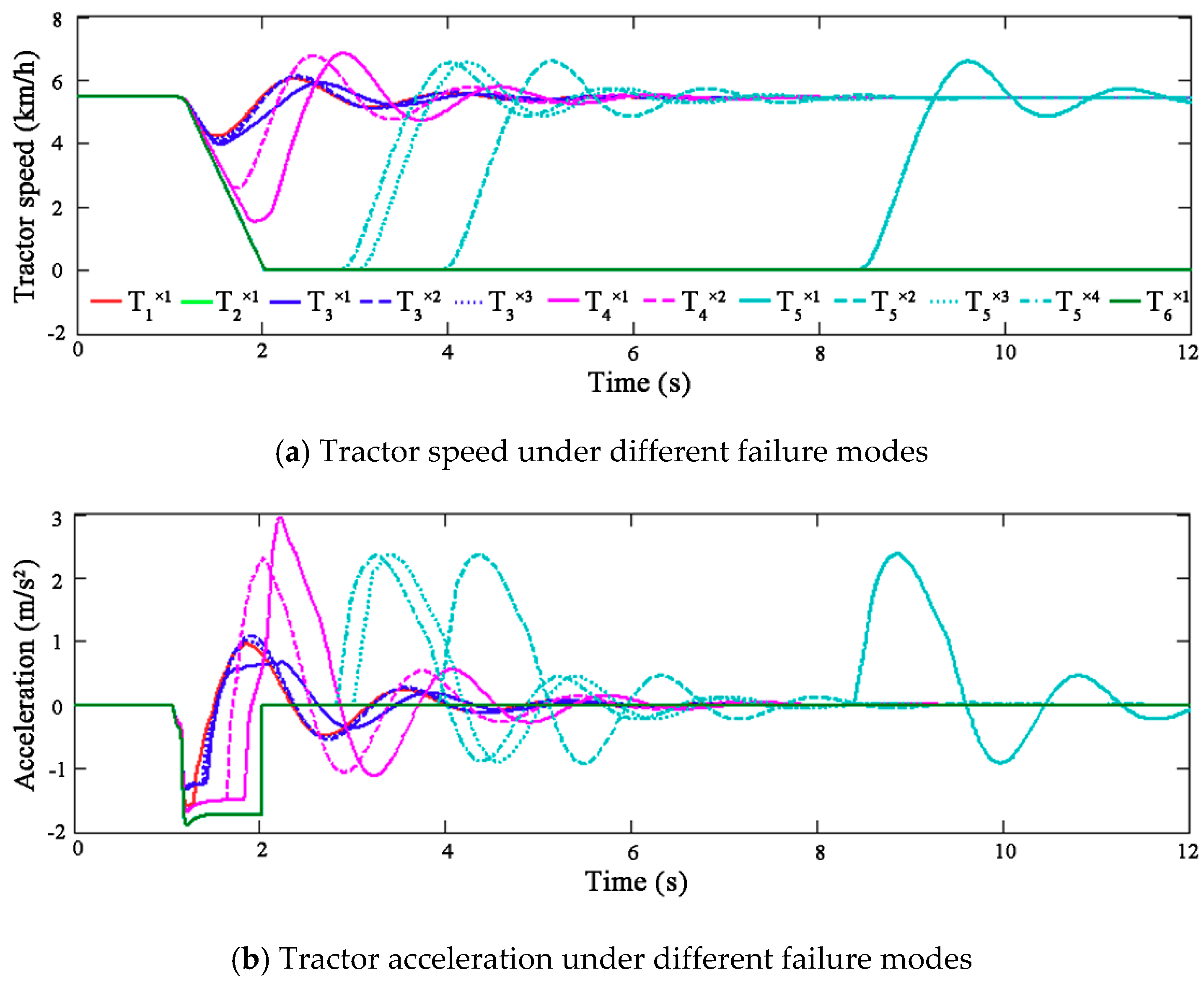
4.4. Effect of Failure Mode on Shifting Quality

Based on the oil pressure corresponding to T₁–T₆, the response speed and acceleration of the tractor, as well as the power loss and energy loss of the clutch were calculated as shown in Figure 13a–d, respectively.

It can be seen from the figure that when the tractor shifted in normal mode T₁, the speed drop was 1.243 km/h, the peak acceleration 0.961 m/s², the maximum power loss 2.276 kW, and the accumulated energy loss 0.9611 kJ. By contrast:

(1) The tractor had power interruption in failure modes T₂, T₅, and T₆. In particular, with the slow recovery of oil pressure, failure mode T₅ made the tractor suddenly recover its power after stopping. This process not only violated the driver’s operation intention and brought great driving risk, but also produced large tractor peak acceleration (up to 2.381 m/s²), high instantaneous power loss (up to 47.47 kW), and large accumulated energy loss (up to 34.26 kJ).

(2) Although the failure mode T₃ may cause the shifting quality to decline, it could still ensure the normal driving of the tractor. In the failure mode T₃, the speed drop was 1.498 km/h, the peak acceleration 1.087 m/s², the maximum power loss 7.71 kW, and the accumulated energy loss 3.991 kJ.

(3) Although the failure mode T₄ did not make the tractor shutdown, it resulted in poor shifting quality of tractor. In failure mode T₄, the speed drop was 3.939 km/h, the peak acceleration 2.962 m/s², the maximum power loss 31.07 kW, and the accumulated energy loss 13.46 kJ.

5. Conclusions

In this paper, a method of fault analysis for the hydrostatic power split CVT was proposed. By building a simulation model, the risk degree of some faults could be predicted without damaging the transmission. The specific conclusions were as follows:

(1) The mathematical model constructed in this paper could accurately calculate the response of the hydrostatic power split CVT to the clutch engagement pressure.

(2) The damage of the seal ring inside the rotary joint had little effect on shifting quality. Sometimes, it could even reduce the acceleration impact of the tractor during shift, but it increased the energy loss of the clutch.

(3) Oil way blockage could lead to greater shift acceleration impact and clutch energy loss.

(4) When seal ring damage and oil way blockage occurred together, the clutch oil pressure could not reach the minimum working pressure, which would lead to power interruption, and the tractor could not work normally.

(5) Clutch piston jamming and oil leakage could cause power interruption of the tractor. These were all serious hydraulic system failures.

As mentioned above, the simulation method based on this study could predict the effect of fault oil pressure on the shifting quality of tractor, but it could not reveal the causal relationship between the fault of hydraulic system and the shape of the oil pressure curve. As one of the important works in the future, the formation mechanism of hydraulic system fault should be studied.

References

1. Xia, Y.; Sun, D. Characteristic analysis on a new hydro-mechanical continuously variable transmission system. Mech. Mach. Theory 2018, 126, 457–467. [Google Scholar] [CrossRef]
2. Renius, K.T.; Resch, R. Continuously variable tractor transmissions. In Proceedings of the Agricultural Equipment Technology Conference, Louisville, KY, USA, 14–16 February 2005; ASAE: Joseph, MI, USA, 2005; pp. 1–37. [Google Scholar]
3. Rossetti, A.; Macor, A.; Benato, A. Impact of control strategies on the emissions in a city bus equipped with power-split transmission. Transp. Res. Part D 2017, 50, 357–371. [Google Scholar] [CrossRef]
4. Rossetti, A.; Macor, A. Multi-objective optimization of hydro-mechanical power split transmissions. Mech. Mach. Theory 2013, 62, 112–128. [Google Scholar] [CrossRef]
5. Ni, X.; Zhu, S.; Ouyang, D.; Chang, Y.; Wang, G.; Thinh, N.V. Design and experiment of hydro-mechanical CVT speed ratio for tractor. Trans. Chin. Soc. Agric. Mach. 2013, 44, 15–20. [Google Scholar]
6. Li, B.; Sun, D.; Hu, M.; Zhou, X.; Liu, J.; Wang, D. Coordinated control of gear shifting process with multiple clutches for power-shift transmission. Mech. Mach. Theory 2019, 140, 274–291. [Google Scholar] [CrossRef]
7. Oh, J.; Park, J.; Cho, J.; Kim, J.; Kim, J.; Lee, G. Influence of a clutch control current profile to improve shift quality for a wheel loader automatic transmission. Int. J. Precis. Eng. Manuf. 2017, 18, 211–219. [Google Scholar] [CrossRef]
8. Raikwar, S.; Tewari, V.K.; Mukhopadhyay, S.; Verma, C.R.B.; Rao, M.S. Simulation of components of a power shuttle transmission system for an agricultural tractor. Comput. Electron. Agric. 2015, 114, 114–124. [Google Scholar] [CrossRef]
9. Hajjaji, A.E.; Chadli, M.; Oudghiri, M.; Pages, O. Observer-based robust fuzzy control for vehicle lateral dynamics. In Proceedings of the 2006 American Control Conference, Minneapolis, MN, USA, 14–16 June 2006; pp. 4664–4669. [Google Scholar]
10. Wang, R.; Jing, H.; Hu, C.; Chadli, M.; Yan, F. Robust H∞ output-feedback yaw control for in-wheel motor driven electric vehicles with differential steering. Neurocomputing 2016, 173, 676–684. [Google Scholar] [CrossRef]
11. Wang, G.; Chadli, M.; Chen, H.; Zhou, Z. Event-triggered control for active vehicle suspension systems with network-induced delays. J. Frankl. Inst. 2019, 356, 147–172. [Google Scholar] [CrossRef]
12. Repin, S.; Evtiukov, S.; Maksimov, S. A method for quantitative assessment of vehicle reliability impact on road safety. Transp. Res. Procedia 2018, 36, 661–668. [Google Scholar] [CrossRef]
13. Feng, G.; Hou, Y.; Sun, H. Simulation analysis of the gear shift buffer of the armored vehicles. Comput. Simul. 2018, 35, 7–11. [Google Scholar]
14. Wei, C.; Ma, Z.; Yin, X.; Zhao, J.; Li, X. Research on the influencing factors of the range-shifting impact on HMT. Trans. Beijing Inst. Technol. 2015, 35, 1122–1127. [Google Scholar]
15. Zhang, M.; Hao, X.; Yin, Y. Neural network PID control for mulit-range hydro-mechanical continuously variable transmission in tractors. J. Henan Polytech. Univ. 2017, 36, 93–98. [Google Scholar]
16. Wang, G.; Zhu, S.; Shi, L.; Wang, S.; Zhang, H.; Nguyen, V. Control and interaction system for tractor hydro-mechanical CVT. Trans. Chin. Soc. Agric. Mach. 2015, 46, 1–7. [Google Scholar]
17. Park, S.; Kim, S.; Choi, J.H. Gear fault diagnosis using transmission error and ensemble empirical mode decomposition. Mech. Syst. Signal Process. 2018, 108, 262–275. [Google Scholar] [CrossRef]
18. Huang, Y.; Huang, C.; Ding, J.; Liu, Z. Fault diagnosis on railway vehicle bearing based on fast extended singular value decomposition packet. Measurement 2019, in press. [Google Scholar] [CrossRef]
19. Chang, X.; Tang, B.; Tan, Q.; Deng, L.; Zhang, F. One-dimensional fully decoupled networks for fault diagnosis of planetary gearboxes. Mech. Syst. Signal Process. 2019, in press. [Google Scholar] [CrossRef]
20. Rao, Z. Design of Planetary Gear Transmission, 1st ed.; Chemical Industry Press Co., Ltd.: Beijing, China, 2003; p. 27. [Google Scholar]
21. Shi, J. Design of Hydro-Mechanical Continuously Variable Transmission Used on the Unroad Vehicle and Research on the Control System of Variable Pump. Master’s Thesis, Nanjing Agricultural University, Nanjing, China, April 2012. [Google Scholar]
22. Walker, P.; Zhu, B.; Zhang, N. Powertrain dynamics and control of a two speed dual clutch transmission for electric vehicles. Mech. Syst. Signal Process. 2017, 85, 1–15. [Google Scholar] [CrossRef] [Green Version]
23. Meng, F.; Tao, G.; Chen, H. Smooth shift control of an automatic transmission for heavy-duty vehicles. Neurocomputing 2015, 159, 197–206. [Google Scholar] [CrossRef]
24. Zhao, Z.; Jiang, S.; Ni, R.; Fu, S.; Han, Z.; Yu, Z. Fault-tolerant control of clutch actuator motor in the upshift of 6-speed dry dual clutch transmission. Control Eng. Pract. 2020, 95, 104268. [Google Scholar] [CrossRef]
25. Iqbal, S.; Bender, F.A.; Ompusunggu, A.P.; Pluymers, B.; Desmet, W. Modeling and analysis of wet friction clutch engagement dynamics. Mech. Syst. Signal Process. 2015, 60, 420–436. [Google Scholar] [CrossRef]
26. ITI GmbH. ITI SimulationX Help Manual; ITI GmbH: Dresden, Germany, 2012. [Google Scholar]
27. Xu, X.; Han, X.; Liu, Y.; Liu, Y.; Liu, Y. Modeling and dynamic analysis on the direct operating solenoid valve for improving the performance of the shifting control system. Appl. Sci. 2017, 7, 1266. [Google Scholar] [CrossRef] [Green Version]
28. Li, W.; Abel, A.; Todtermuschke, K.; Zhang, T. Hybrid vehicle power transmission modeling and simulation with SimulationX. In Proceedings of the International Conference on Mechatronics and Automation, Harbin, China, 5–8 August 2007; pp. 1710–1717. [Google Scholar]
29. Tai, J. Design of the 2×2 Type HMCVT of Large Power Tractor and Study on the Shift Quality of HMCVT. Master’s Thesis, Shandong Agricultural University, Taian, China, June 2017. [Google Scholar]
30. Duncan, J.R.; Wegscheid, E.L. Determinants of off-road vehicle transmission ‘shift quality’. Appl. Ergon. 1985, 16, 173–178. [Google Scholar] [CrossRef]
Figure 1. Schematic diagram of the hydrostatic power split CVT.
Applsci 10 00681 g001
Figure 2. Schematic diagram of clutch hydraulic control system.
Applsci 10 00681 g002
Figure 3. Output speed of the CVT at different engine speeds and displacement ratios. PV, variable displacement pump; MF, fixed displacement motor.
Applsci 10 00681 g003
Figure 4. Distribution of equivalent moment of inertia.
Applsci 10 00681 g004
Figure 5. Schematic diagram of the spring-damper model.
Applsci 10 00681 g005
Figure 6. Structure of the wet clutch.
Applsci 10 00681 g006
Figure 7. Schematic diagram of friction plates transmitting torque under normal force.
Applsci 10 00681 g007
Figure 8. Dynamic model of the CVT tractor.
Applsci 10 00681 g008
Figure 9. Test bench of the power shift for the hydrostatic power split CVT.
Applsci 10 00681 g009
Figure 10. Test verification of the transmission model.
Applsci 10 00681 g010
Figure 11. Oil pressure curve of clutch C2 in different failure modes.
Applsci 10 00681 g011
Figure 12. Clutch damaged due to failure mode T2.
Applsci 10 00681 g012
Figure 13. Shifting quality of the CVT tractor under different failure modes.
Applsci 10 00681 g013aApplsci 10 00681 g013b