Reducing Dynamic Power Consumption in Mixed-Critical Real-Time Systems

Abstract

In this paper, we study energy minimization consumption of a mixed criticality real-time system on uni-core. Our focus is on a new scheduling scheme to decrease the frequency level in order to conserve power. Since many systems are equipped with dynamic power and frequency level memory, power can be saved by decreasing the system frequency. In this paper, we provide new dynamic energy minimization consumption in mixed-criticality real-time systems. Recent research has been done on low-criticality mode for power reduction. Thus, the proposed scheme can reduce the energy both in high-criticality and low-criticality modes. The effectiveness of our proposed scheme in energy reduction is clearly shown through simulations results.

1. Introduction

Real-time systems take some inputs and produce outputs in a time-bound manner. Meeting deadline is the core concept of a real-time system such that missing a deadline may collapse the whole system. A real-time system has fragile uses such as an airline command system, which is so highly critical that a single failure can cause a major explosion. Similarly, a real-time system is employed in satellite receivers for collecting highly important information and failures can misguide and result in a major collapse [1]. Daily home appliances such as microwave, AC, electric power system, and refrigerator, etc. can also employ a real-time system.

In a real-time system, the term mixed-critically means that high-critical tasks must meet their deadlines at the cost of missing deadlines for certain low-criticality tasks. Therefore mixed-criticality can be used as a tool for assuring the system failure needed for different components. In the literature, mixed-criticality is identified as mission-criticality and LO- (low-criticality) criticality. The mission-criticality (hard real-time) failures can cause major damage in the systems such as loss of flight control, receiving wrong information via radar system, and misguiding satellite data. On the other hand, LO-criticality (soft real-time) is relaxed critical and can be considered less destructive such that deadlines can be violated occasionally.

A mixed-criticality system $\left(MCS\right)$ is characterized to execute in each of two modes, high and low critical mode [2]. Each task is described by the shortest arrival time of a task (period denoted by P), deadline (denoted by D), and Worst case execution time $WCET$ one per criticality level, denoted by $(C_i\left(LO\right)$ and $C_i\left(HI\right)$. The condition of the basic $MCS$ model is the system beginning in the LO-criticality mode and can stay in that mode given all jobs execute within their low-criticality computation times $(C_i\left(LO\right)$. If any job executes for its $(C_i\left(LO\right)$ execution time without any signal, the system directly moves to high-criticality (HI)-criticality mode. In HI-criticality mode, LO-criticality jobs should not be executed but some level of service should be maintained if at all possible as LO-criticality tasks are still critical.

In this scheme Guan, Emberson, and Pedro [3,4,5] consider a simple protocol for mode switch situations for controlling the time of the change of mode back to low-criticality, which is to wait until the CPU is idle and then safely be made. Producing a somewhat more efficient scheme, Santy [6] extends this approach that can be applied to a globally scheduling multi-processor system in which the CPU may never get to an ideal tick. In a dual criticality level that has just shifted into a HI-criticality mode and hence no LO-criticality tasks are computed, its protocol is to first wait when the HI-criticality task has completed its high computation time and then wait for the next high priority task, and this continues until the lowest priority job is inactive and it is then safe to reintroduce all low-criticality jobs. If there is a further misbehavior of low computation bound the protocol drops all low-criticality jobs if any jobs compute more then its $(C_i\left(LO\right)$ value.

Dynamic voltage and frequency scaling (DVFS) is a commonly-used technique for reducing the overall energy consumption, which is minimized in a large-scale data processing environment. This technique is based on utilizing two common parameters such as processor voltage and processor frequency to reduce power consumption. DVFS enable processor maximum power consumption, which can be accomplished by decreasing the operating frequency level of a processor. However, a scale-down of the processor’s CPU frequency causes a delay in task completion time. Much of the literature has been focused on reducing power consumption in embedded systems. A similar technique, real-time dynamic voltage and frequency scaling (RT-DVFS), studied reducing power consumption for periodic and aperiodic tasks. In the RT-DVFS technique, slack time is used as a parameter for adjusting the processor speed such that tasks deadlines will be guaranteed.

In the proposed work, we scheduled a single-processor which support variable frequency and voltage scaling. Our aim is to schedule the given jobs that a CPU speeds all jobs achieved to meet its deadline and minimize energy. Few research has been done on minimizing the energy in a mixed-criticality (MC) real-time system, in [7] CPU acceleration is a deterioration algorithm that adds for given mixed-criticality aperiodic real-time tasks. They characterize an optimization issue of power consumption in MC real-time systems under extended frequency scaling. As the same time each job is performed under the derived frequency scaling. So we enhanced the dynamic approach where the frequency level accommodates under the derived frequency scaling for the plain power decline. The main grant in this research is that we reduced energy in HI-criticality mode dynamically.

2. Related Work and Problem Description

Initially, an MC system is considered by Vestal [8] for scheduling and since then it has gained increasing interest in real-time scheduling. S. Barauch and P. Ekberg consider [9] the mixed-criticality system in a way that all LO-criticality jobs are discarded when the system mode switches to HI-criticality [10,11,12]. In [13], they showed that the scheme of Vestal is optimal for fixed-priority scheduling systems. In [14], they provided response-time analysis of mixed-criticality tasks in order to increase the schedulability of fixed-priority tasks. In [10], they provided a heuristic scheduling algorithm based on Audsley priority assignment strategy for efficient scheduling.

Audsley approach [15] is used to assign priority from the lowest to highest level. At each priority level, the lowest priority job from the low criticality task set is tried first, if it is schedulable then the job moves up to the next priority level if it is schedulable, then the lowest search can be abandoned as the task set is unscheduled. In [16], they considered how these time-triggered tables can be produced via first simulation.

The energy-minimization consumption of a processor is generally classified into dynamic and static techniques in terms of the consideration of dynamic frequency adjustment. They are also classified into continuous or discrete frequency level schemes according to the assumption of frequency continuity. Yao et al. [17] and Aydin et al. [18] also proposed a static (or offline) scheduling method to reduce energy minimization in a real-time system, in this paper [19] Jejurikar and Gupta study the energy saving of a periodic real-time job. Gruian determined proposed stochastic data to derive a energy-efficient schedules scheme in [20]. In [21], they provided minimum power consumption in periodic task scheduling for discrete frequency-level systems. On the contrary, the dynamic scheduling scheme adjusts the CPU frequency or speed levels depending on the current system load in order to fully utilized the CPU slack time.

The Audsley scheme for assigning priority to mixed-criticality jobs is based on their criticality level in this paper [15], and priority is given to jobs manner high to low scheduling priorities so that priorities are given to lowest priorities task, the schedule difficulty of the MC real-time system is investigated by Baruah, the author proof when all jobs are released at the same time is when these jobs are set to NP-complete [9]. In this scheme, they investigated the optimal schedule algorithm for the MC system scheduling performing well in practice.

The own criticality base priority (OCBP) to MC sporadic jobs by Li and Baruah [22] considers criticality for priority assignment. When a new job arrives to the system, a new priority is assigned to the job. In [3], they presented a scheduling scheme known as priority-list reuse scheduling based on the OCBP scheduler. In [23], they assumed a likewise realistic energy model and presented an optimal static scheme for minimizing the energy of multi-component with adjusting individual frequencies main memory and processor system bus.

The connection between multiple-choice knap sack problem (MCKP) and dynamic voltage scaling (DVS) for periodic task and energy optimization was at first proven by Mejia-Alvarez and Mosse [24]. In this paper Aydin et al. consider [18] the dynamic voltage frequency scaling scheme for periodic jobs that complete before their worst-case execution times (WCETs). In [25], they proposed the elastic scheduling for the purpose of utilizing CPU with discrete frequencies. In [26], they presented a dynamic slack algorithm allocation for real time that consider both the loss energy minimization and frequency scaling overhead. The cycle conservation approach was proposed by Mei et al. [27]. They suggested a novel power aware scheduling scheme named cycle conservation DVFS for sporadic jobs. In this algorithm P.Pillai and K.G.Shin [28] proposed real-time DVS, the OS’s real time scheduler, and jobs managing service to allocate minimum power consumption while maintaining that the deadlines must always be met.

More recently researches on a power-aware mixed-criticality real-time system have been presented by [7,29]. The major technique is used for a power-aware mixed-criticality system and they consider only a set job with no periodical jobs. They determine possible CPU speed degraded for MCS jobs. In this algorithm [29], they show that minimizing the energy of power-aware mixed-criticality real-time scheduling for periodic jobs under continuous frequency scaling. The early deadline first with the virtual deadline (EDF-VD) algorithm [11] provide the most favorable virtual deadline (VD) and frequency scaling of jobs, and do not adjust during run time the derived frequency levels of jobs. In [30], when high-critical jobs do not finish low computation time, all low-critical jobs are terminated and the system frequency level is set to maximum, in this paper they only reduce frequency in low-critical mode.

In our work we provide an efficient power-aware scheduling algorithm in MC real-time systems and adjust the optimal frequency level of high-criticality mode, to the best of our knowledge this is the first work that introduces optimal energy consumption of high-criticality mode in a mixed-criticality real-time system, the main grant our scheme is that we minimize energy in high-criticality mode dynamically and show the experimental results in simulations.

3. System Model

3.1. Task Model

In this subsection, we provide an overview of the task model. In the mixed-criticality real-time systems, a low-criticality periodic task releases an order of jobs only in low criticality mode, while high-criticality tasks release their jobs in both high- and low-criticality mode. Thus a mixed-criticality task ${\tau }_i$ consists of four parameters: Period $\left(P_i\right)$, computation time of low-criticality jobs, $C_i\left(LO\right)$, computation time of high-criticality jobs, $C_i\left(HI\right)$, and tasks level $\left(X_i\right)$ as follows:

• $P_i$: The task period. The task releases a job every period (minimum interval arrival time);
• $C_i\left(LO\right)$: The worst-case execution time in low-criticality mode. The task requires $C_i\left(LO\right)$ times in low-criticality mode;
• $C_i\left(HI\right)$: The worst-case execution time in high-criticality mode. The task requires $C_i\left(HI\right)$ times in high-criticality mode;
• $X_i$: The criticality level of task. The system can be either in high-criticality (HI) mode or in low-criticality (LO) mode.

The task ${\tau }_i$ is a periodic real-time task, so that jobs are released at every $P_i$ time units. The j-th instance or job of a task ${\tau }_i$ is denoted as the ${\tau }_{i,j}$. In the mixed-criticality system, tasks are categorized into low-criticality and high-criticality tasks. In addition, the system mode is also divided into low-criticality and high-criticality mode. In low-criticality mode, all tasks release their jobs so that each task’s job ${\tau }_i$ requires the worst-case execution time of $C_i\left(LO\right)$. On the contrary, in high-criticality mode, only the high-criticality tasks release their jobs with $C_i\left(HI\right)$ execution time ($C_i\left(HI\right)\le C_i\left(LO\right)$). Thus, each task has its criticality mode $X_i$.

The mixed-criticality system is an integrated suit of hardware, middleware service, operating system, and application software that support the execution of non-criticality, mission-criticality, and safety-critical functions. The system starts in low-criticality mode. However, if there is a possibility that any low-critical job interrupts in high-criticality jobs’ execution time, then the system criticality mode changes. In such a situation, all low-criticality tasks are dropped in the system. In mixed-criticality systems, such a possibility occurs when a high-criticality job does not complete its computation time, which is the condition of switching from low-criticality mode to high-criticality mode.

On the contrary, the system returns to low-criticality mode when there is no possibility of overrun. While high-criticality tasks are executed in high-criticality mode, the system changes its criticality to low mode as long as there is no task ready in the queue [29].

For example, Figure 1 shows an example of three mixed-criticality tasks of ${\tau }_1$(2, 2, 5, LO), ${\tau }_2$(1, 3, 6, HI), and ${\tau }_3$(2, 3, 8, HI). The system starts in low-criticality mode, where each task requires $C_i\left(LO\right)$ execution time. Each task releases its job every $P_i$ time units. The scheduling algorithm used in Figure 1 is EDF (earliest deadline first).

Figure 1. An example of mixed-criticality scheduling.

Let us assume that the job ${\tau }_{3,3}$ does not complete its execution at time 19. Then, the system changes the criticality mode to high-criticality. After then, the system executes only high-criticality tasks (${\tau }_2$ and ${\tau }_3$) with their $C_i\left(HI\right)$ execution times. The execution times of ${\tau }_{3,3}$ and ${\tau }_{2,4}$ become 3 in each. When the system is in high-criticality mode, all low-criticality jobs are ignored or removed from the queue. For instance, the job ${\tau }_{1,5}$ released at time 20 is removed from the scheduling queue since it is a low-criticality job.

The systems returns to low-criticality mode if there is no high-criticality jobs waiting in the scheduling queue. For example, the system returns back to the low-criticality mode at time 23 because there are no jobs available. After then, the system executes low-criticality jobs again as before.

3.2. Power Model

In this paper, we assume the DVFS-enabled CPU system where the CPU frequency is adjusted dynamically during run-time. The number of discrete frequency levels is given by m while the frequency levels are defined as a set F.

Let us assume that a task requires t execution time on the CPU at its maximum frequency level. For a given frequency level f of the CPU, the relative speed level s is defined by $f/f_{\max }$, where $f_{\max }$ is the maximum frequency level. Then, the task execution time is defined by $t/s$.

Since the dynamic power consumption is a major issue in the power consumption of systems, we take dynamic power consumption into account in the paper. Generally, the dynamic power is in proportion to $f^3$ or $f^4$ for a frequency level f, we use Equation (1) for the execution time model of a task with t execution time on the relative speed level s [31].

$$E=\alpha ·\frac{t}{s}·s^3=\alpha ·t·s^2,$$

(1)

where $\alpha$ is a coefficient. In this paper we assume $\alpha =1$ for the sake of simplicity.

Figure 2 shows an DVFS scheme for real-time task scheduling. For example, a real-time task requires 3 time unit for its execution, while its result requires 10 time units (Figure 2a). If there is no other task, the system has 7 time-unit slack time to the task deadline. Thus, the task can be executed on the relative speed level of 0.3, as shown in Figure 2b. In the reduced CPU speed level, the system can reduce the power consumption without violating the task deadline.

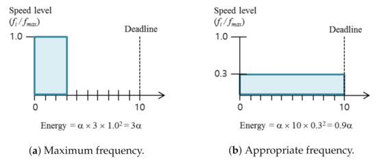
Figure 2. Dynamic voltage scaling (DVS) for real-time tasks.

4. Research Motivations

4.1. Recap of EDF-VD for Power-Aware Mixed-Criticality Real-Time Tasks

In this subsection, we describe a brief explanation of the previous work on power-aware mixed-criticality tasks scheduling [29]. The base scheduling algorithm is early deadline first with the virtual deadline (EDF-VD) which is a mode-switched EDF scheduling technique developed for mixed-criticality task sets [22,32,33]. The reservation of time budgets for $HI$ criticality tasks is done in the $LO$ mode. This is achieved by shortening the deadline of $HI$ criticality tasks. Intuitively, shortening the deadline of $HI$ criticality tasks will push them to finish earlier in the $LO$ mode, leaving more time until their actual deadlines to accommodate extra workloads. Indeed, this form of safety preparation (i.e., shortening deadlines of $HI$ criticality tasks in the $LO$ mode) has proven to be effective in improving system schedulability [34].

In EDF-VD, the value of x in a system determines the virtual deadline $V{D}_i$ as $P_i·x$, where $0<x\le 1$. In order to guarantee the schedulability of task sets both in LO mode and HI mode, the value of x should satisfy the two equations of Equations (2) and (3):

$$\frac{U_{LO}^{HI}}{x}+U_{LO}^{LO}\le 1$$

(2)

$$U_{HI}^{HI}+x{U}_{LO}^{LO}\le 1$$

(3)

In [29], EDF-VD is adjusted in order to provided power-awareness for mixed-criticality real-time systems. They defined a problem of power-aware scheduling in MC systems. The objective is to minimize power consumption satisfying both Equations (4) and (5):

$${\displaystyle \sum _{{\tau }_i\in T_{HI}}\frac{C_i\left(LO\right)/f_{LO}^{HI}}{P_i}}·\frac{1}{x}+{\displaystyle \sum _{{\tau }_i\in T_{LO}}}\frac{C_i\left(LO\right)/f_{LO}^{LO}}{P_i}\le 1$$

(4)

$${\displaystyle \sum _{{\tau }_i\in T_{HI}}}\frac{C_i\left(HI\right)}{P_i}+x·{\displaystyle \sum _{{\tau }_i\in T_{LO}}}\frac{C_i\left(LO\right)/f_{LO}^{LO}}{P_i}\le 1$$

(5)

where $T_{HI}$ and $T_{LO}$ are sets of high-criticality tasks and low-criticality tasks, in each. In Equations (4) and (5), $f_{LO}^{LO}$ and $f_{LO}^{HI}$ indicate optimal frequency levels of HI-criticality tasks and LO-criticality tasks in low mode. They provided an optimal solution to derive x, $f_{LO}^{LO}$, and $f_{LO}^{HI}$ for the formulated problem.

For example, Table 1 shows an example of a task set. The optimal values of $x,f_{LO}^{LO}$, and $f_{LO}^{HI}$ are given by 0.56, 0.6, and 0.8, respectively from the method in [29]. The right three columns of Table 1 shows the virtual deadline and the execution time in low-criticality mode. Figure 3 shows the scheduling example of Table 1 based on EDF-VD.

Table 1. An example of tasks.

Task	${\mathit{P}}_{\mathit{i}}$	${\mathit{C}}_{\mathit{i}}\left(\mathit{LO}\right)$	${\mathit{C}}_{\mathit{i}}\left(\mathit{HI}\right)$	${\mathit{X}}_{\mathit{i}}$	${\mathit{VD}}_{\mathit{i}}=\mathit{x}·{\mathit{P}}_{\mathit{i}}$	${\mathit{C}}_{\mathit{i}}\left(\mathit{LO}\right)/{\mathit{f}}_{\mathit{LO}}^{\mathit{LO}}$	${\mathit{C}}_{\mathit{i}}\left(\mathit{HI}\right)/{\mathit{f}}_{\mathit{LO}}^{\mathit{HI}}$
${\tau }_1$	6	1	2	HI	3.36	-	1.25
${\tau }_2$	8	1	3	HI	4.48	-	1.25
${\tau }_3$	12	1	1	LO	-	1.67	-
${\tau }_4$	16	2	2	LO	-	2.33	-

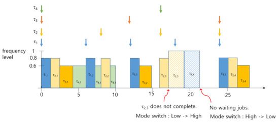
Figure 3. An example of power-aware mixed-criticality Scheduling of Table 1.

As shown in Figure 3, high-criticality tasks, ${\tau }_1$ and ${\tau }_2$, are run at a $f_{LO}^{HI}$ frequency level in low-criticality mode, while low-criticality tasks of ${\tau }_3$ and ${\tau }_4$ run at $f_{LO}^{LO}$. Let us assume that ${\tau }_{2,3}$ does not complete $C_i\left(LO\right)$ at time 17.25. Then, the system mode changes to high-criticality mode so that two low-criticality jobs of ${\tau }_3$ and ${\tau }_4$ are ignored after the mode switch event. In high-criticality mode, the frequency level is set as the maximum frequency in order to guarantee the schedulability of high-criticality tasks. The system mode returns back to low-criticality mode after executing all high-criticality jobs.

4.2. Motivations

As discussed in the previous subsection, the previous work focused on low-criticality mode. However, we can further reduce the power in high-criticality mode without violating the schedulability. For example, we can reduce the frequency level while executing ${\tau }_{2,3}$ and ${\tau }_{1,4}$ in the high-criticality mode of Figure 3.

In order to guarantee the schedulability in both criticality modes, we need appropriate frequency levels in each mode. The main problem of this paper is to determine optimal frequency levels that consider both modes.

5. The Proposed Scheme

5.1. Dynamic Power Aware Scheme MCS Jobs

The proposed scheme dynamically adjusts the CPU frequency level depending on both the system mode and task mode. The baseline frequency levels are derived from static analysis so that x, $f_{LO}^{LO}$, $f_{LO}^{HI}$, and $f_{HI}^{HI}$ are obtained before run-time. Throughout the optimization problem, we solve those values in the initial step.

The power-consumption with consideration of both high- and low-crticality modes in defined by the following three equations. The unit-time power consumption in low-crticality mode is derived by Equation (6), where $LCM$ is the least common multiplier of all periods. In Equation (6), the total power consumption during $LCM$ is computed by adding the power consumption of task ${\tau }_i$ in low mode using Equation (1). The number of ${\tau }_i$’s jobs is $LCM/P_i$. Thus, the unit-time power consumption is obtained by dividing the total sum with $LCM$.

Similarly, the unit-time power consumption in high-criticality mode is defined by Equation (7). Thus, the average unit-time power consumption can be obtained as the expected value in each mode, as in Equation (8), where $P_{LO}$ and $P_{HI}$ denote the probabilities of the system mode in low- and high-crticality, respectively.

$$\begin{array}{ccc}\hfill U{P}_{LO}& =& \frac{1}{LCM}\left(\sum _{{\tau }_i\in T_{LO}}\frac{LCM}{P_i}·\frac{C_i\left(LO\right)}{f_{LO}^{LO}}·{\left(f_{LO}^{LO}\right)}^3+\sum _{{\tau }_i\in T_{HI}}\frac{LCM}{P_i}·\frac{C_i\left(LO\right)}{f_{LO}^{HI}}·{\left(f_{LO}^{HI}\right)}^3\right)\hfill \\ & =& \sum _{{\tau }_i\in T_{LO}}\frac{C_i\left(LO\right)}{P_i}·{\left(f_{LO}^{LO}\right)}^2+\sum _{{\tau }_i\in T_{HI}}\frac{C_i\left(LO\right)}{P_i}·{\left(f_{LO}^{HI}\right)}^2\hfill \\ & =& U_{LO}^{LO}·{\left(f_{LO}^{LO}\right)}^2+U_{LO}^{HI}·{\left(f_{LO}^{HI}\right)}^2\hfill \end{array}$$

(6)

$$\begin{array}{ccc}\hfill U{P}_{HI}& =& \frac{1}{LCM}\sum _{{\tau }_i\in T_{HI}}\frac{LCM}{P_i}·\frac{C_i\left(HI\right)}{f_{HI}^{HI}}·{\left(f_{HI}^{HI}\right)}^3\hfill \\ & =& \sum _{{\tau }_i\in T_{HI}}\frac{C_i\left(HI\right)}{P_i}·{\left(f_{HI}^{HI}\right)}^2\hfill \\ & =& U_{HI}^{HI}·{\left(f_{HI}^{HI}\right)}^2\hfill \end{array}$$

(7)

$$\begin{array}{ccc}\hfill UAP& =& U{P}_{LO}·P_{LO}+U{P}_{HI}·P_{HI}\hfill \\ & =& \left(U_{LO}^{LO}·{\left(f_{LO}^{LO}\right)}^2+U_{LO}^{HI}·{\left(f_{LO}^{HI}\right)}^2\right)·P_{LO}+U_{HI}^{HI}·{\left(f_{HI}^{HI}\right)}^2·P_{HI}\hfill \end{array}$$

(8)

For the given probabilities of $P_{LO}$ and $P_{HI}$, the problem of deciding the optimal frequency levels and x of EDF-VD is: to minimize

$$\left(U_{LO}^{LO}·{\left(f_{LO}^{LO}\right)}^2+U_{LO}^{HI}·{\left(f_{LO}^{HI}\right)}^2\right)·P_{LO}+U_{HI}^{HI}·{\left(f_{HI}^{HI}\right)}^2·P_{HI}$$

(9)

subject to

$$\frac{U_{LO}^{HI}}{f_{LO}^{HI}}·\frac{1}{x}+\frac{U_{LO}^{LO}}{f_{LO}^{LO}}\le 1$$

(10)

$$\frac{U_{HI}^{HI}}{f_{HI}^{HI}}+x·\frac{U_{LO}^{LO}}{f_{LO}^{LO}}\le 1.$$

(11)

The scheduling system flow in low mode is shown in Figure 4a. Each task releases jobs with $C_i\left(LO\right)$ execution time every period. Since we use EDF-VD, the virtual deadline of a high-criticality job released at time t is given by $t+V{D}_i$. The deadline of low-criticality job is set as $t+p_i$. These new jobs are waiting in the ready queue.

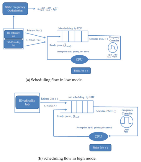
Figure 4. The proposed scheduling framework.

The scheduling algorithm for jobs is based on early deadline first so that the job with the earliest deadline is scheduled first. At the time of dispatching a high-criticality job, the CPU frequency level is set as $f_{LO}^{HI}$. On the contrary, the frequency level is adjusted with $f_{LO}^{LO}$ for low-criticality job execution.

When a high-criticality job does not complete its low-mode execution time, then the system switches to high-criticality mode. At that time, all low-criticality jobs are dropped in order to guarantee high-criticality tasks as shown in Figure 4b. However, the system can switch back to low-mode at any time when there is no pending task.

5.2. DVFS Scheduling

The notation for the scheduling algorithm is shown in Table 2. The task utilization of ${\tau }_i$ is denoted as $U_i$. Each job, denoted as $J_k$, in the waiting queue is defined by ($C_k$, $D_k$) so that a job requires $C_k$ execution time by the deadline $D_k$. The values are determined at the time of job release.

Table 2. Notations.

Notation	Meaning
$U_i$	The utilization of the task ${\tau }_i$
$J_k=(C_k,D_k)$	The job of task ${\tau }_i$
t	The current time
${\mathcal{Q}}_{ready}$	The CPU ready queue
$J_{curr}$	current job of execution

The proposed scheme is defined by functions that are called at a certain event. The algorithms are given in the followings pseudo-code in Algorithms 1 and 2.

• Job-Release (${\tau }_i$): Every $P_i$ period, a task ${\tau }_i$ releases a job. The function Job-Release is called;
• Job-Finish ($J_i$): The function is called when a job completes its execution or over-runs the execution time;
• Power-aware Schedule (): At the time of a job release or completion, the function re-schedules jobs in the queue;
• Frequency-Adjust (): The CPU frequency is adjusted at the time of job allocation to the CPU.

When a job is released in low mode, the job is inserted in the ready queue. The task utilization is also updated. Since the frequency-level of a LO-criticality task is given by $f_{LO}^{LO}$, the task utilization is determined by the equation in line 5 of Algorithm 1. In case of a high-critical job of $C_i\left(HI\right)-C_i\left(LO\right)$ every period so that the utilization is given by the equation in line 7. If the current system mode is low, we terminate or ignore the low-criticality job. If the current mode is high, we execute the high-criticality job (line 14). The job is inserted in the ready queue, we call the scheduling algorithm in line 19.

When the job $J_i$ finishes its computation, if the current system mode is low, nothing is executed. We only check $X_i$ = HI. We have two cases if $J_i$ finishes. If $J_i$ does not complete, the system mode becomes high. When the ready queue is empty and there is no high-criticality job in the ready queue, the system mode is changed from high to low (lines 29–31).

The function Power-aware Schedule () dispatches jobs using EDF (line 38–43 of Algorithm 1). At each scheduling event, Frequency-Adjust () function is called so as to adjust the CPU frequency dynamically. As shown in Algorithm 2, if the system is in high-criticality mode, we minimize the frequency of high-criticality mode which is set as $f_{HI}^{HI}$. The frequency level is set as the frequency level sufficient to schedule current jobs. Thus, the relative speed level of the frequency is greater than or equal to the current utilization.

Algorithm 1 Algorithm of energy minimization consumption in mixed-criticality tasks.
1:	functionJob-Release(${\tau }_i$)
2:	if the current system mode is Low then
3:	Insert job $J_i(C_i\left(LO\right),t+V{D}_i)$ into ${\mathcal{Q}}_{ready}$
4:	if $X_i=$ Low then	▹ Low-criticality job
5:	$U_i\leftarrow (C_i\left(LO\right)/f_{LO}^{LO})/P_i$
6:	else
7:	$U_i\leftarrow (C_i\left(LO\right)/f_{LO}^{HI})/P_i$ + $((C_i\left(HI\right)-C_i\left(LO\right)/f_{HI}^{HI})/P_i$
8:	end if
9:	else	▹ The current system mode is High
10:	if $X_i=$ Low then
11:	$U_i\leftarrow$ 0
12:	else	▹$X_i=$ High
13:	$U_i\leftarrow (C_i\left(HI\right)/f_{HI}^{HI})/P_i$
14:	Insert job $J_i(C_i\left(HI\right),t+P_i)$ into ${\mathcal{Q}}_{ready}$
15:	end if
16:	end if
17:	Power-aware Schedule()
18:	end function
19:	functionJob-Finish($J_i$)
20:	if the current system mode is Low then
21:	if $X_i=$ High then	▹ High-criticality job
22:	if $J_i$ finish $C_i\left(LO\right)$ completely then
23:	$U_i\leftarrow (Ci\left(LO\right)/f_{LO}^{HI})/P_i$
24:	else
25:	The system mode changed to High	▹ Mode switch to HI
26:	end if
27:	end if
28:	else	▹ The current system mode is High
29:	if ${\mathcal{Q}}_{ready}=⌀$ then
30:	The system mode is changed from High to Low	▹ Mode switch back to LO
31:	end if
32:	end if
33:	Power-aware Schedule()
34:	end function
35:	functionPower-aware Schedule()
36:	if ${\mathcal{Q}}_{ready}\ne ⌀$ then
37:	$J_k\leftarrow$ the job with the earliest deadline in ${\mathcal{Q}}_{ready}$
38:	if $J_{curr}=⌀$then	▹ CPU idle
39:	$J_{curr}\leftarrow J_k$
40:	else if $D_k<D_{curr}$then	▹ Preemption by EDF
41:	$J_{curr}$ is preempted and re-Inserted into ${\mathcal{Q}}_{ready}$
42:	$J_{curr}\leftarrow J_k$
43:	end if
44:	Frequency-Adjust()
45:	end if
46:	end function

Algorithm 2 Algorithm of selecting frequency.

1: functionFrequency-Adjust() 2:     if The system is in High mode then 3:         The frequency is set as $f_{HI}^{HI}$. 4:     else        ▹The system is in Low mode. 5:         $U\leftarrow min({\sum }_{i=1}^n{U}_i,1.0)$ 6:         if $X_{curr}=$ LO then 7:            $U\leftarrow U\times f_{LO}^{LO}$ 8:         else 9:            $U\leftarrow U\times f_{LO}^{HI}$ 10:         end if 11:         freq ← the minimum $f_i\in \mathcal{F}$ s.t. $U\le f_i/f_{max}$ 12:         The frequency is set as freq. 13:     end if 14: end function

5.3. Example

Let us consider the task set in Table 1 as an example. The previous work derives the optimal value of $f_{LO}^{LO}$ and $f_{LO}^{HI}$ as 0.6 and 0.8, respectively. In high-criticality mode, the maximum frequency level is used. However, the proposed work derives the optimal frequency levels by solving Equation (9) with two constraints of Equations (10) and (11). Table 3 shows those values for given probabilities of high- and low-criticality mode.

Table 3. Optimal frequency levels and x of the example of Table 1.

		x	${\mathit{f}}_{\mathit{LO}}^{\mathit{LO}}$	${\mathit{f}}_{\mathit{LO}}^{\mathit{HI}}$	${\mathit{f}}_{\mathit{HI}}^{\mathit{HI}}$	Power Improvement
Previous		0.56	0.6	0.8	1	-
Previous	$P_{HI}=0.1$	0.56	0.6	0.8	1	0%
	$P_{HI}=0.2$	0.52	0.7	0.8	0.9	1.5%
	$P_{HI}=0.3$	0.47	0.7	0.9	0.8	6.3%
	$P_{HI}=0.4$	0.47	0.7	0.9	0.8	14.6%

For example, for a given $P_{HI}=0.2$, the optimal frequency levels of $f_{LO}^{LO}$, $f_{LO}^{HI}$, and $f_{HI}^{HI}$ are 0.7, 0.8, and 0.9. The scheduling example of Table 1 in the same scenario as Figure 3 is shown in Figure 5. The frequency level in high-criticality is set as 0.9, not as 1.0. As shown in Table 3, the proposed work can reduce more energy in higher probability of high-criticality mode.

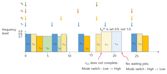
Figure 5. An example of proposed power-aware scheduling.

6. Performance Evaluation

6.1. Simulations Environment

We conduct extensive simulation to validate the proposed idea by utilizing random power-aware mixed-criticality task sets. Simulation parameters are shown in Table 4. We used six discrete frequency levels in the system. The execution time is randomly generated from 1 to 100. Then, the task period is defined in order to meet the target utilization. We have a different utilization of LO- and HI-criticality jobs which is 0.2, 0.25, 0.3, 0.35, 0.4, and 0.45. We have five different tasks in a set, where the numbers of LO-criticality and HI-criticality tasks are two and three in each. We generate 1000 random tasks sets to evaluate the effect of energy minimization consumption for a given tasks sets. We simulate each task set for the least common multiple of the tasks’ periods.

Table 4. Simulation Parameters.

Parameters	Values
CPU Frequency levels	0.4, 0.5, 0.6, 0.7, 0.8, 0.9, 1.0
$U_{LO}^{LO}$	0.3, 0.35, 0.4, 0.45
$U_{LO}^{HI}$	0.3, 0.35, 0.4, 0.45,
Low-to-high rate (r)	1.5, 2.0, 2.5, 3.0
Low-criticality tasks	2
High-criticality tasks	3

6.2. Energy Consumption Results

We present energy consumption for different task sets as shown in Figure 6a–d. We measure the average value of 1000 task sets. The figure presents energy consumption as a function of system utilization for different probabilities. As shown in the figure, the proposed approach achieves better minimum energy consumption compared to that of existing approaches for the same task set. The main reason of minimum energy consumption is due to the task utilization at low and high criticality modes. The figure further shows that when the probability of high-criticality mode is increased, the impact of energy consumption gradually increases from 0.01 to 0.09. As shown in Figure 6c, the minimum energy consumption depends on the probability values for task utilization U = (0.2, 0.25, 0.3, 0.35, 0.4, 0.45).

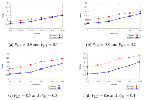
Figure 6. Average energy results.

We also present the impact of average x on energy minimization in Figure 7. We consider the same value of x for both previous and proposed approaches. When the value of utilization is increased by 0.35, the proposed approach achieves significant improvement in the performance. The impact of x in the probabilities is shown in Figure 7a. When the utilization is between 0.2 and 0.25, the average x is 0.4 but when the utilization is increased up to 0.35 and the value of x is increased by 0.56. When the utilization is between 0.35 and 0.4, then the average value of x goes to 0.65. This implies that in HI-criticality mode the energy consumption is not affected when we increase the value of x.

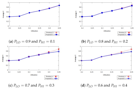
Figure 7. The impact of x.

Figure 8 shows energy consumption as a function of different ratios of low- and high-computation times. The figure considers different values of r ranging from 1.5 to 3. The ratio between low-critical and high-critical execution time in the sequence in order to observe its effects on the scheduling of mixed-criticality tasks. As shown in Figure 8, the increasing ratio also leads to an increase in the average energy consumption. When the ratio is 1.5, the values of average energy for proposed and previous approaches are 0.082 and 0.136, respectively. Similarly, when the probability is between 0.6 to 0.4, the proposed approach minimizes energy consumption as compared to that of the previous approach as shown in Figure 8b. It is concluded that an increase in the ratio leads to increase in the average energy consumption of the mixed-criticality task sets.

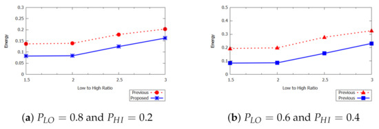
Figure 8. The impact of ratio r.

The result in Figure 9 shows the impact of different task sets in mixed-criticality systems. The figure presents the average energy as a function of seven task sets, i.e., (1LO/6HI, 2LO/5HI, 3LO/4HI, 4LO/3HI, 5LO/2HI, 6LO/1HI) ranging from low to high critical modes. It is observed that the average energy is increasing for the average number of 1000 task sets.

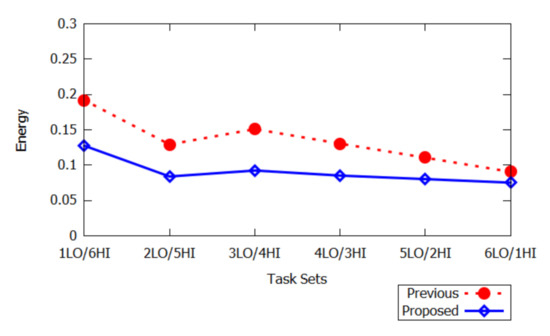
Figure 9. Impact of the number of low- and high-criticality tasks ($P_{HI}=0.2$).

In Figure 10, the average energy consumption is presented for different frequency intervals. The figure shows the effects of the task-sets frequencies on minimum energy consumption. In the range between 0.4 and 0.5, we generate random task sets utilization for the sufficient number of tasks. When the frequency interval is between 0.05 and 1, the proposed approach outperforms the previous approach approach. Figure 10b shows that when the frequency interval is between 0.05 and 0.1, the value of x decreases. It is concluded that the proposed approach achieves a lower value of x compared to that of the previous approach.

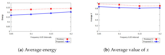
Figure 10. Impact of frequency intervals.

6.3. Comparison Summary

The following Table 5 describes a comparison with the previous work. Although the previous work sets the maximum frequency level in high-criticality mode, the proposed scheme adjusts the level. When the probability of high-criticality mode is low, the performance of both work seems similar. However, the proposed work has more overhead for frequency scaling adjustment.

Table 5. Comparison summary.

	Previous	Proposed
Frequency in HI-mode	Maximum	Optimized
Performance at low $P_{HI}$	Near optimal	Optimal
Performance at high $P_{HI}$	Good	Optimal
Frequency switch overhead	Moderate	High

7. Discussion and Conclusions

7.1. Discussion

An issue of the proposed work is practicality in terms of the probability of high-criticality mode. Recent work [35,36] have considered the probability of execution times of tasks for mixed-criticality systems. In [37], they introduced the probabilistic confidence of a task and a system and provided statistical scheduling algorithm. In [35,36], probabilistic scheduling algorithms are analyzed for mixed-criticality real-time systems with a consideration of mode-switch probabilities.

As shown in Figure 6a, the proposed work shows the similar performance in low-$P_{HI}$ systems. When the probability of high-criticality mode is extremely low (e.g., ${10}^{-8}$), the effect of power reduction in high-criticality mode is negligible. However, the proposed work is still useful in terms of followings.

• Although the probability of mode-switch of an individual task is low, the probability of the system mode-switch can be increased for a larger number of tasks. Let us assume that $f_i$ is defined by the probability of the task’s ${\tau }_i$ mode-switch. Then, the probability of the system mode-switch of the task set T is derived by $1-{\Pi }_{{\tau }_i\in T}(1-f_i)$ [35]. Figure 11 shows the probability of the system mode-switch in terms of individual task’s probability and the number of tasks (N). Let us note that the x-axis in Figure 11 is log-scale. In case of $N=50$, the proposed work may affect the performance from the probability of task mode-switch of 0.002 because the proposed work shows performance gain where $P_{HI}\ge 0.1$. On the contrary, when the number of tasks is higher (e.g., $N=200$), the probability of system mode-switch will become higher from lower task mode-switch probability (e.g., $f_i=0.001$). Thus, the proposed work will be useful depending on the number of tasks and task’s mode-switch probability;
  

  Figure 11. The probability of mode switch w.r.t. task mode switch probability and the number of tasks.
• The system mode-switch policy also affects the probability. In mixed-criticality systems, it is still an open issue on how long the system remains in high-criticality mode after the mode-switch occurrence. The proposed work performance is useful in mixed-criticality systems where the system should remain for a certain period after the mode-switch;
• Finally, the problem formulation with consideration of high-criticality mode is one contribution. Since the probability of mode-switch can be adjusted according to the system safety requirement, the proposed work will be useful when the system optimization is required in mixed-criticality systems.

7.2. Concluding Remark

In this paper, we designed a new dynamic power-aware scheduling scheme of mixed-criticality real-time tasks under high frequency scaling on unicore processors. To tackle the difficulty in trading off minimizing power in HI-criticality mode to reduce the overall average energy, we first proposed reducing the energy level in high-criticality mode. Furthermore, we switched to low-critical mode if there was idle time between high critical job executions.

Our experimental simulation results show that our scheme is more efficient in terms of reducing energy at the high critical mode as well as in low critical mode. Our proposed scheme outperformed the static scheme for reducing energy because the frequency scaling in the static scheme may not have been optimal in dynamic scheme. The results validated that our proposed scheme better performed by increasing the probability of the high critical tasks in comparison to low critical tasks.

We plan to investigate more on the proposed scheduling scheme and extend it to the multi-core processor systems. In addition, we will further analyze the probability of high-criticality mode in many applications and apply it to the proposed work. We will also apply the probabilistic scheduling approach in the proposed work in order to find the optimal power-aware scheduling.

References

- Aeronautical Radio Inc. Avionics Application Software Standard Interface Part 1 Required Services; ARINC Specification 653P1-2; Aeronautical Radio Inc.: Annapolis, MD, USA, December 2005. [Google Scholar]
- Burns, A.; Davis, R. Mixed Criticality Systems-A review. In Proceedings of the 2011 IEEE 32nd Real-Time Systems Symposium, Vienna, Austria, 29 November–2 December 2011; pp. 1–69. [Google Scholar]
- Guan, N.; Ekberg, P.; Stigge, M.; Yi, W. Effective and Efficient Scheduling of Certifiable Mixed-Criticality Sporadic Task Systems. In Proceedings of the 2011 IEEE 32nd Real-Time Systems Symposium, Vienna, Austria, 29 November–2 December 2011; pp. 13–23. [Google Scholar]
- Emberson, P.; Bate, I. Minimising Task Migration and Priority Changes in Mode Transitions. In Proceedings of the 13th IEEE Real Time and Embedded Technology and Applications Symposium, Bellevue, WA, USA, 3–6 April 2007; pp. 158–167. [Google Scholar]
- Pedro, P.; Burns, A. Schedulability Analysis for Mode Changes in Flexible Real-Time Systems. In Proceedings of the 10th Euromicro Workshop on Real-Time Systems, Berlin, Germany, 17–19 June 1998; pp. 172–179. [Google Scholar]
- Santy, F.; Raravi, G.; Nelissen, G.; Nelis, V.; Kumar, P.; Goossens, J.; Tovar, E. Two Protocols to Reduce The Criticality Level of Multiprocessor Mixed-Criticality Systems. In Proceedings of the 21st International Conference on Real-Time Networks and Systems, Sophia Antipolis, France, 17–18 October 2013; pp. 183–192. [Google Scholar]
- Baruah, S.; Guo, Z. Mixed-Criticality Scheduling upon Varying-speed Processors. In Proceedings of the 2013 IEEE 34th Real-Time Systems Symposium, Vancouver, BC, Canada, 3–6 December 2013; pp. 68–77. [Google Scholar]
- Vestal, S. Preemptive Scheduling of Multi-Criticality Systems with Varying Degrees of Execution Time Assurance. In Proceedings of the 28th IEEE International Real-Time Systems Symposium, Tucson, AZ, USA, 3–6 December 2007; pp. 239–243. [Google Scholar]
- Baruah, S.; Bonifaci, V.; D’Angelo, G.; Li, H.; Marchetti-Spaccamela, A.; Megow, N.; Stougie, L. Scheduling Real-Time Mixed-Criticality Jobs. IEEE Trans. Comput. 2012, 61, 1140–1152. [Google Scholar] [CrossRef]
- Baruah, S.K.; Burns, A.; Davis, R.I. Response-Time Analysis for Mixed Criticality Systems. In Proceedings of the 2011 IEEE 32nd Real-Time Systems Symposium, Vienna, Austria, 29 November–2 December 2011; pp. 34–43. [Google Scholar]
- Baruah, S.K.; Bonifaci, V.; d’Angelo, G.; Marchetti-Spaccamela, A.; Van Der Ster, S.; Stougie, L. Mixed-Criticality Scheduling of Sporadic Task Systems. In Proceedings of the European Symposium on Algorithms, Saarbrücken, Germany, 5–9 September 2011; pp. 555–556. [Google Scholar]
- Baruah, S.; Vestal, S. Schedulability Analysis of Sporadic Tasks with Multiple Criticality Specifications. In Proceedings of the 2008 Euromicro Conference on Real-Time Systems, Prague, Czech Republic, 2–4 July 2008; pp. 147–155. [Google Scholar]
- Dorin, F.; Richard, P.; Richard, M.; Goossens, J. Schedulability and Sensitivity Analysis of Multiple Criticality Tasks with Fixed-Priorities. Real Time Syst. 2010, 46, 305–331. [Google Scholar] [CrossRef]
- Baruah, S.; Li, H.; Stougie, L. Towards The Design of Certifiable Mixed-Criticality Systems. In Proceedings of the 2010 16th IEEE Real-Time and Embedded Technology and Applications Symposium, Stockholm, Sweden, 12–15 April 2010; pp. 13–22. [Google Scholar]
- Audsley, N.C. Optimal Priority Assignment and Feasibility of Static Priority Tasks with Arbitrary Start Times; Department of Computer Science, University of York: York, UK, 1991. [Google Scholar]
- Socci, D.; Poplavko, P.; Bensalem, S.; Bozga, M. Time-Triggered Mixed-Critical Scheduler on Single and Multi-Processor Platforms. In Proceedings of the 2015 IEEE 17th International Conference on High Performance Computing and Communications, New York, NY, USA, 24–26 August 2015; pp. 684–687. [Google Scholar]
- Yao, F.; Demers, A.; Shenker, S. A Scheduling Model for Reduced CPU Energy. In Proceedings of the IEEE 36th Annual Foundations of Computer Science, Milwaukee, WI, USA, 23–25 October 1995; pp. 374–382. [Google Scholar]
- Aydin, H.; Melhem, R.; Mossé, D.; Mejía-Alvarez, P. Power-aware Scheduling for Periodic Real-Time Tasks. IEEE Trans. Comput. 2004, 53, 584–600. [Google Scholar] [CrossRef]
- Jejurikar, R.; Gupta, R. Optimized Slowdown in Real-time Task Systems. IEEE Trans. Comput. 2006, 55, 1588–1598. [Google Scholar] [CrossRef]
- Gruian, F. Hard Real-Time Scheduling for Low-Energy using Stochastic Data and DVS Processors. In Proceedings of the 2001 International Symposium on Low Power Electronics and Design, Huntington Beach, CA, USA, 6–7 August 2001; pp. 46–51. [Google Scholar]
- Zhong, X.; Xu, C.Z. System-Wide Energy Minimization for Real-Time Tasks: Lower Bound and Approximation. ACM Trans. Embed. Comput. Syst. 2008, 7, 1–24. [Google Scholar] [CrossRef]
- Li, H.; Baruah, S. An Algorithm for Scheduling Certifiable Mixed-Criticality Sporadic Task Systems. In Proceedings of the 2010 31st IEEE Real-Time Systems Symposium, San Diego, CA, USA, 30 November–3 December 2010; pp. 183–192. [Google Scholar]
- Yun, H.; Wu, P.L.; Arya, A.; Kim, C.; Abdelzaher, T.; Sha, L. System-Wide Energy Optimization for Multiple DVS Components and Real-Time Tasks. Real Time Syst. 2011, 47, 489–515. [Google Scholar] [CrossRef]
- Mejia-Alvarez, P.; Levner, E.; Mossé, D. Adaptive Scheduling Server for Power-Aware Real-Time Tasks. ACM Trans. Embed. Comput. Syst. 2004, 3, 284–306. [Google Scholar] [CrossRef]
- Marinoni, M.; Buttazzo, G. Elastic DVS Management in Processors with Discrete Voltage/Frequency Modes. IEEE Trans. Ind. Inform. 2007, 3, 51–62. [Google Scholar] [CrossRef]
- Wang, W.; Ranka, S.; Mishra, P. Energy-Aware Dynamic Slack Allocation for Real-Time Multitasking Systems. Sustain. Comput. Inform. Syst. 2012, 2, 128–137. [Google Scholar] [CrossRef]
- Mei, J.; Li, K.; Hu, J.; Yin, S.; Sha, E.H.M. Energy-Aware Preemptive Scheduling Algorithm for Sporadic Tasks on DVS Platform. Microprocess. Microsyst. 2013, 37, 99–112. [Google Scholar] [CrossRef]
- Pillai, P.; Shin, K.G. Real-Time Dynamic Voltage Scaling for Low-Power Embedded Operating Systems. In Proceedings of the Eighteenth ACM Symposium on Operating Systems Principles, Banff, AB, Canada, 21–24 October 2001; pp. 89–102. [Google Scholar]
- Huang, P.; Kumar, P.; Giannopoulou, G.; Thiele, L. Energy Efficient DVFS Scheduling for Mixed-Criticality Systems. In Proceedings of the 2014 International Conference on Embedded Software, Jaypee Greens, India, 12–17 October 2014; pp. 1–10. [Google Scholar]
- Ijaz, A.; Jun-ho, S.; Kyong, H.K. A Dynamic Power-aware Scheduling of Mixed-Criticality Real-time Systems. In Proceedings of the 2015 IEEE International Conference on Computer and Information Technology, Ubiquitous Computing and Communications; Dependable, Autonomic and Secure Computing; Pervasive Intelligence and Computing, Liverpool, UK, 26–28 October 2015; pp. 438–445. [Google Scholar]
- Niu, L.; Quan, G. Reducing Both Dynamic and Leakage Energy Consumption for Hard Real-Time Systems. In Proceedings of the 2004 International Conference on Compilers, Architecture, and Synthesis for Embedded Systems, Washington, DC, USA, 22–25 September 2004; pp. 140–148. [Google Scholar]
- Ekberg, P.; Yi, W. Bounding and Shaping The Demand of Generalized Mixed-Criticality Sporadic Task Systems. Real Time Syst. 2014, 50, 48–86. [Google Scholar] [CrossRef]
- Liu, D.; Spasic, J.; Guan, N.; Chen, G.; Liu, S.; Stefanov, T.; Yi, W. EDF-VD Scheduling of Mixed-Criticality Systems with Degraded Quality Guarantees. In Proceedings of the 2016 IEEE Real-Time Systems Symposium, Porto, Portugal, 29 November–2 December 2016; pp. 35–46. [Google Scholar]
- Baruah, S.; Bonifaci, V.; D’Angelo, G.; Li, H.; Marchetti-Spaccamela, A.; Van Der Ster, S.; Stougie, L. The Preemptive Uniprocessor Scheduling of Mixed-Criticality Implicit-Deadline Sporadic Task Systems. In Proceedings of the 2012 24th Euromicro Conference on Real-Time Systems, Pisa, Italy, 11–13 July 2012; pp. 145–154. [Google Scholar]
- Guo, Z.; Santinalli, L.; Yang, K. EDF Schedulability Analysis on Mixed-Criticality Systems with Permitted Failure Probability. In Proceedings of the 21st IEEE International Conference on Embedded and Real-Time Computing Systems and Applications (RTCSA), Hong Kong, China, 19–21 August 2015. [Google Scholar]
- Maxim, D.; Davis, R.I.; Cucu-Grosjean, L.; Easwaran, A. Probabilistic Analysis for Mixed Criticality Systems using Fixed Priority Preemptive Scheduling. In Proceedings of the 25th International Conference on Real-Time Networks and Systems, Grenoble, France, 4–6 October 2017. [Google Scholar]
- Edgar, S.; Burns, A. Statistical analysis of WCET for scheduling. In Proceedings of the 2001 IEEE Real-Time Systems Symposium, London, UK, 3–6 December 2001. [Google Scholar]
Publisher’s Note: MDPI stays neutral with regard to jurisdictional claims in published maps and institutional affiliations. |
© 2020 by the authors. Licensee MDPI, Basel, Switzerland. This article is an open access article distributed under the terms and conditions of the Creative Commons Attribution (CC BY) license (http://creativecommons.org/licenses/by/4.0/).