Offensive and Defensive Plus–Minus Player Ratings for Soccer


Faculty of Logistics, Molde University College, 6410 Molde, Norway
Appl. Sci. 2020, 10(20), 7345; https://doi.org/10.3390/app10207345
Submission received: 15 September 2020
/
Revised: 9 October 2020
/
Accepted: 16 October 2020
/
Published: 20 October 2020
(This article belongs to the Special Issue Computational Intelligence and Data Mining in Sports)
Abstract
:Rating systems play an important part in professional sports, for example, as a source of entertainment for fans, by influencing decisions regarding tournament seedings, by acting as qualification criteria, or as decision support for bookmakers and gamblers. Creating good ratings at a team level is challenging, but even more so is the task of creating ratings for individual players of a team. This paper considers a plus–minus rating for individual players in soccer, where a mathematical model is used to distribute credit for the performance of a team as a whole onto the individual players appearing for the team. The main aim of the work is to examine whether the individual ratings obtained can be split into offensive and defensive contributions, thereby addressing the lack of defensive metrics for soccer players. As a result, insights are gained into how elements such as the effect of player age, the effect of player dismissals, and the home field advantage can be broken down into offensive and defensive consequences.
1. Introduction
Soccer has become a large global business, and significant amounts of capital are at stake when the competitions at the highest level are played. While soccer is a team sport, the attention of media and fans is often directed towards individual players. An understanding of the game therefore also involves an ability to dissect the contributions of individual players to the team as a whole.
Plus–minus ratings are a family of player ratings for team sports where the performance of the team as a whole is distributed to individual players. Such ratings have been successfully used by media for sports such as ice hockey and basketball, and creators of such rating systems work as analysts for National Basketball Association (NBA) teams, influencing their decisions on trades and free-agent signings [1]. There has recently been several academic contributions towards plus–minus ratings for soccer [2], although the influence of these ratings has not yet reached the same levels as in basketball.
The most trivial form of plus–minus, which originated in ice hockey during the 1950s [1], is to count the number of goals scored minus the number of goals conceded when a given player is in the game. This form, however, fails to take into account the effects of teammates and the opposition. Therefore, in the context of basketball, Winston [3] used linear regression to create adjusted plus–minus ratings, where the plus–minus score of each player is adjusted for the effects of the other players on the court. The main drawback of this approach is that individuals that always play together cannot be discerned, and rating estimates become extremely unreliable. Sill [4] solved this by introducing a regularized adjusted plus–minus rating for basketball, where the linear regression model is estimated using ridge regression, introducing a bias and reducing the variance of the rating estimates.
Most often, plus–minus ratings are taken as an overall performance measure. However, some research has been done where the ratings are split into an offensive and a defensive contribution. This paper presents a new plus–minus rating for soccer, where each player is given an offensive and a defensive rating, based on how the player contributes towards creating and preventing goals, respectively. The motivation for this work is to see whether splitting the player ratings into offensive and defensive components can lead to additional insights about the contributions of individual players, teams, and leagues. If successful, this could be useful for an initial phase of data-driven scouting at clubs, to better identify a list of prospective players for recruitment. The urgency of properly identifying both offensive and defensive contributions was illustrated in the context of basketball by Ehrlich et al. [5]. They provided an analysis, based on offensive and defensive plus–minus ratings, to show that win-maximizing teams in the NBA can reduce their expenses by hiring defensively strong players.
The new rating system is evaluated on a data set containing more than 52 thousand matches played from 2008 to 2017. The rating model is used to evaluate the effect of age on player performance, the home field advantage, the relative quality of different leagues, and the difference in performance of players in different positions on the field. Each of these are examined from the perspective of offensive and defensive contributions. Furthermore, rankings of players and teams as of July 2017 are presented and discussed, illustrating how the offensive and defensive ratings can be used to indicate interesting differences between players. The new offensive–defensive plus–minus rating appears to be the most complete rating of this type for soccer provided in the academic literature as of yet.
The remainder of this paper is structured as follows. Section 2 summarizes the current literature on plus–minus ratings. The new offensive–defensive plus–minus rating for soccer is then described in Section 3. This is followed by an explanation of how the ratings are tested and evaluated in Section 4. Then, Section 5 presents the detailed results, after which concluding remarks are given in Section 6.
2. Literature Review
The first academic work on plus–minus ratings in soccer was published by Sbø and Hvattum [6]. They presented a regularized adjusted plus–minus rating, in which ridge regression is used in the estimation of a multiple linear regression model, with variables representing the presence of players on each team, the home field advantage, and player dismissals. Observations in the model were generated from maximal segments of matches where the set of players on the pitch remained unchanged. In other words, new segments are started at the beginning of a match, for every substitution made and for every red card given. The dependent variable is taken as the difference between the number of goals scored by the home team and the away team within the segment.
Sbø and Hvattum [7] suggested an improvement of the regression model, adding variables representing the current league and division of the players, allowing player ratings to better reflect the differences in strength between league systems and league divisions. Kharrat et al. [8] presented a similar model, but experimented with three different dependent variables: the difference in goals scored, the difference in scoring probabilities for shots (expected goals), and the change in the difference in expected points.
Around this time, Hvattum [2] provided a thorough review of the literature on plus–minus ratings for team sports. Early non-academic discussions of such ratings for soccer include the writings of Bohrmann [9] and Hamilton [10]. In addition, similar player ratings were developed by Sittl and Warnke [11], Vilain and Kolkovsky [12], and Schultze and Wellbrock [13]. Matano et al. [14] followed the main structure of Sbø and Hvattum [7] and Kharrat et al. [8], but used computer game ratings as a Bayesian prior for the plus–minus ratings, avoiding the problem of ridge regression driving all player ratings towards zero. Volckaert [15] implemented a plus–minus rating similar to that of Sbø and Hvattum [7] which was tested on data from the Belgium top division. The ratings obtained were shown to be a significant predictor of players’ market values, despite being based on a relatively small data set. In addition to ratings based on a regularized multiple linear regression, Volckaert [15] also tested ratings calculated from a regularized Poisson model. The latter resulted in seemingly different rankings, but was not analyzed further.
Pantuso and Hvattum [16] continued the work of Sbø and Hvattum [7], improving several aspects of the model, including a better handling of red cards and the home field advantage. However, the two most important enhancements were in adding an age component to the players’ ratings, as well as replacing the regularization of player ratings with a penalty that moves the rating of a player towards the average rating of the player’s teammates. The resulting ratings were analyzed by Gelade and Hvattum [17] and Arntzen and Hvattum [18]. The former found that simple key performance metrics for players were reasonably related to the plus–minus ratings, while the latter showed that plus–minus player ratings could add important information to team ratings when predicting match outcomes.
The line of work culminating with the ratings of Pantuso and Hvattum [16] only considered the goal difference of a segment as the dependent variable, and only created a single overall rating for each player. Vilain and Kolkovsky [12], however, considered both offensive and defensive plus–minus ratings for soccer. Their ratings are based on an ordered probit regression, where two observations are generated for each match: one considering the goals scored by the home team, and one considering the goals scored by the away team. The latent variable is assumed to depend linearly on variables representing the offensive ratings of players on the focal team and the defensive ratings of the opposing team. Their calculations explicitly prevented defenders from having an offensive rating, forwards from having a defensive rating, and goalkeepers from having any rating. The work is also described in [19].
In plus–minus ratings for other team sports, it is more common to consider both offensive and defensive ratings for each player. For basketball, Rosenbaum [20] made the first mention of splitting plus–minus ratings into offensive and defensive components. Witus [21] suggested that this was done by first estimating total plus–minus ratings, and then running a second regression to determine the proportion of each player’s value to come from their offense and their defense. Ilardi and Barzilai [22] presented an alternative where offensive and defensive ratings were estimated directly, with observations for each possession. Fearnhead and Taylor [23] considered observations consisting of intervals without substitutions. Their model includes both offensive and defensive ratings, and has separate home advantage parameters for the offensive and defensive contributions, with the dependent variable being the number of points scored per possession. Ratings are assumed to be drawn from Gaussian distributions, and the hyperparameters estimated by maximum likelihood indicates that players are more similar in terms of defensive ability than offensive ability. Kang [24] proposed to use penalized logistic regression to estimate offensive and defensive ratings for NBA players. With observations based on single possessions, the logistic regression estimates the probabilities of scoring, given the players appearing and an offensive home field advantage, while using L2 (ridge) regularization.
For ice hockey, the first contribution towards offensive and defensive plus–minus ratings was made by Macdonald [25], who considered both a single model to estimate offensive and defensive ratings directly as well as the approach of first calculating a single plus–minus rating that is split into offensive and defensive ratings by a second model. In either case, multiple linear regression is used, estimated by the method of ordinary least squares. The work was extended in [26] to cover power play situations, while Macdonald [27] used ridge regression and alternative dependent variables. The latter was extended further in [28]. Thomas et al. [29] defined hazard functions for the scoring rates of each team, yielding offensive and defensive player ratings. The model was applied only to full-strength situations.
3. New Offensive–Defensive Plus–Minus Ratings
The new rating model aims to estimate offensive and defensive ratings for each player. These ratings are entirely data driven, and are defined so that the sum of the offensive ratings of the home team minus the sum of the defensive ratings of the away team should approximately equal the number of goals scored by the home team. Similarly, the number of goals scored by the away team should be approximately equal to the sum of the offensive ratings of the away team minus the sum of the defensive ratings of the home team. However, the goals scored and conceded by the home team are also expected to vary depending on the home field advantage and the number of player dismissals. The ratings of players are not assumed to be constant over time, but rather to be a function of the player’s age: young players tend to be improving over time, while the playing strength of older players tend to decline.
Considering a part of a match where the players are fixed, ratings are determined by minimizing the squared difference between the actual number of goals scored and the number of goals expected based on the players’ ratings, other effects such as the home field advantage, and the duration of a segment. Hence, the numerical values of the ratings obtained are interpreted as the contribution of a player towards goals scored per 90 min. To calculate ratings, data must be available regarding the starting line-ups of both teams, the time of goals, red cards, and substitutions, as well as the players involved in red cards and substitutions. Furthermore, the new ratings require knowledge about the birth date of players and their playing position.
3.1. Rating Model
Following Pantuso and Hvattum [16], the new offensive–defensive plus–minus ratings for soccer are calculated by solving an unconstrained quadratic program. Let M be a set of matches, with each match divided into segments , defined as a maximal period of time without changes to the players appearing on the pitch. The duration of segment s is minutes.
Let and be the two teams involved in match m, where h is the home team. In the case that the match is played on neutral ground, one of the two teams is arbitrarily assigned as h and the other as a. Let be the number of goals scored by team h in segment s of match m, whereas the number of goals scored by a is . Past plus–minus rating models have used as the dependent variable of the observation associated to the segment. Here, to facilitate both offensive and defensive ratings, each segment corresponds to two observations. One observation is from the perspective of team h, and has as the dependent variable, whereas the other is from the perspective of a, with as the dependent variable.
In addition, define as the goal difference in favour of h at the beginning of the segment, and as the goal difference at the end of the segment. The change of the goal difference in favour of h in segment s of match m then becomes . Let denote the time that match m is played, and let T be the time at which ratings are calculated, as illustrated in Figure 1.
Let P be the set of all players. The set of players for team t that appears on the pitch for a given segment s are denoted by . The set of players that are involved in offensive contributions is denoted by , and the set of players involved in defensive contributions is denoted by . For , define if team h has received n or more red cards before the beginning of segment s and team a has not, if team a has received n or more red cards and team h has not, and otherwise. If a team has made all its available substitutions and a player on the team becomes injured and must leave the pitch, the situation is modelled in the same way as a red card.
Each match m belongs to a competition organized by an association. Let be the association organizing the match. This could be a national organization, a continental federation such as UEFA, or FIFA. The model allows the home field advantage of match m to depend on . Furthermore, a set of domestic league competitions C is considered, with being the subset of such competitions in which player p has participated. For example, a given player could have appeared in the French Ligue 2, the English Championship, and the English Premier League, resulting in these three leagues being members of .
Each player p is associated to a set of players that are considered to be similar. This set is based on which players have appeared together on the same team for the most minutes of playing time. The time of the last match where players p and appeared together is denoted by (see Figure 1).
The quality of players is assumed to depend on their age, allowing the model to capture their typical improvement in early years as well as their decline when getting older. Let be the time of birth for player p. The age of player p at the time of match m is then , as illustrated in Figure 1. The average effect of age on the ratings of players is modelled as a piecewise linear function. To this end, an ordered set of k age values is defined. For a given match and player, the exact age of the player is expressed as a convex combination of the nearest two ages in Y. Thus, weights , , are defined as
Thus, after censoring so that it lies within , it holds that . In addition, at most two of the values are non-zero, and any two non-zero values are for consecutive values of i. As a concrete example, assuming that , , and , then and uniquely identifies the age of player p at the time of match m.
To improve the calculations of offensive and defensive ratings, a set of positional roles is considered: , where the elements refer to goalkeeper, defender, midfielder, and forward, respectively. Let be the subset of positions covered by player p. This notation is used to improve the distribution of a player’s overall rating into offensive and defensive components, in particular for players with few minutes played.
The following parameters are defined to control the behavior of the model: , , and are regularization factors, with being the main regularization factor, and the others being adjustments made for specific regularization terms. The parameter is a discount factor for older observations, and are parameters regarding the importance of the duration of a segment, while is a parameter for the importance of a segment based on the goal difference at the start and end of the segment. To balance the importance of the age factors when considering similarity of players, the weight is introduced. Finally, is a weight that controls the extent to which overall ratings of players with few minutes played are shrunk towards zero or towards the overall ratings of similar players.
The variables used in the quadratic program can be stated as follows: the offensive base rating of player p is denoted by , and the defensive base rating is ; the value of the home advantage in competitions organized by is represented by and —the former measures the home field advantage in terms of goals scored, and the latter in terms of goals conceded for the home team; for a given age , the age effect is denoted by and for, respectively, the offensive and defensive contribution of a player.
The influence of red cards is also split into an offensive and a defensive contribution, as captured by the variables and for missing players of the home team, and and for missing players of the away team. These variables are defined for . A potential adjustment for player ratings based on the participation in a domestic league competition is given by the variables and . Moreover, is introduced to indicate the average difference between offensive and defensive ratings for players in position .
The model to calculate offensive and defensive plus–minus ratings can now be stated as
The complete model (1)–(8) consists of two main parts: expressions that link the observed number of goals scored and conceded in each segment of each match with the player ratings to be estimated, and regularization terms that are used to guide the estimation of player ratings, in particular for players that are involved in few observations or whose appearances are highly correlated with appearances of other players.
The observations are based on segments that are weighted using . The weights depend on the time since the segment was played, the duration of the segment, and on the goal difference at the start and the end of the segment:
The two observations based on each segment can now be specified in more detail. The quadratic terms in (1) and (2) arise in an attempt to minimize the squared error between a right-hand side consisting of the observed number of goals scored or conceded, and a left-hand side comprising explanatory terms corresponding to players involved in the segment, to attributes of the particular segment, and to attributes of the match to which the segment is associated. The factor is used to scale the explanatory terms so that they can be interpreted as contributions per 90 min of play:
Attributes specific to a segment involve compensating for missing players following red cards and injured platers who are not replaced. For segments of matches where there is a home field advantage present, this is expressed as follows:
However, for matches played on neutral ground, the effect of missing players is modelled as:
Regarding a specific match, the relevant contribution to explain the observed number of goals comes from the home field advantage, which is modelled as being specific to a given association organizing the match:
The remaining terms to explain the observed goals represent the ratings of players at the time of the match. These ratings consist of a base rating plus adjustments based on the age of the player and based on the domestic league competitions where the player has appeared:
The model then includes a set of quadratic terms (3)–(8) known as regularization terms. The purpose of these is to dampen the ratings and other estimated effects, so that very high or very low ratings are avoided for players with few observations in the data set. First, a regularization term ensures that the overall rating of a player is not too different from the overall ratings of similar players:
Second, the following ensures that the difference between the offensive and the defensive rating of a player is not too different from the typical difference for players in similar positions:
The two types of regularization applied above aim to control the player ratings directly. Regularization is not applied to all the other estimates made by the model, such as the home field advantages and the effects of red cards. However, the age effects are subject to regularization, partly to ensure model identifiability, and partly to make sure the age effects are smoothed out when applied to smaller data sets:
The model (1)–(8) constitutes an unconstrained quadratic program. Due to the large dimensions of the problem, a gradient descent search is used to determine its solution. This is coded in C++, and several calculations, such as finding the gradient at a given step, are parallelized over several threads. Once the model has been estimated, the offensive rating of player p at time T corresponds to , while the defensive rating is . The overall rating for player p becomes .
3.2. Example Segment
To illustrate the model, a segment is selected from a match played between Barcelona and Athletic Bilbao in the Spanish Primera División on 17 January 2016. The selected segment of the match started after a substitution in minute 6 and ended with a new substitution in minute 46. Before this, the goalkeeper of the away team had been shown a red card, and the home team had been awarded a penalty shot, which would be taken by Lionel Messi in minute 7. The match was tied when the segment started. The following assumes that the ratings are being estimated on 21 June 2017, and the notation is simplified by dropping references to the match m and the segment s.
The duration of the selected segment is min, and the home team scored twice and the away team zero times during these minutes. The rating model contains two quadratic terms tied directly to this segment, having, respectively, and as the constant terms, representing the goals scored by each team. The weights of the segment become , , and , resulting in .
The number of non-zero linear terms of and , as appearing in the objective function terms (1) and (2), is 44 and 45, respectively. As there is one player sent off for the away team, the segment specific terms are and . The match specific terms represent the home field advantage, with and , with the Spanish league represented by .
As goalkeepers do not have offensive ratings, and since the away team has one player missing, the number of players contributing offensively is and for the two teams, while the number of players contributing defensively is and . These numbers are used to normalize the sum of contributions from player ratings, and , to and .
Table 1 shows the coefficients for the age variables in the selected segment, before scaling by and multiplying by the segment weight w. These coefficients arise from summing over the players appearing in the segment. Based on the coefficients, one can see that the home team has one player aged between 23 and 24, and two players aged between 31 and 32, excluding the goalkeeper: the sum of coefficients for offensive contributions related to age sum up to 1.1 for ages 23 and 24 and to 2.2 for ages 31 and 32, corresponding to the fact that these coefficients have been scaled by 11 and divided by the number of offensive players.
The coefficients of the league components, and are given in Table 2. The players involved in the match had previously appeared in five different league competitions, most commonly being the Spanish Primera División. The away team had six players previously appearing in the Spanish Segunda División, each contributing with and to the given coefficients, with , as these players only appeared in two different league competitions.
Finally, both and have, in total, twenty occurrences of and , representing the main player rating components. With the proposed model, each match is, on average, divided into around 6.3 segments, each of which provides two squared expressions for the objective function. Less than half of the terms in these expression relate directly to player ratings, whereas the rest are used to estimate home field advantages, age effects, and league effects. Taking again the example segment, and focusing on the observation of goals scored by the home team, after factoring in all the weights, the corresponding objective function expression can be stated as
4. Experimental Setup
The data set used to evaluate the rating system and to analyze the values for the estimated parameters, including player ratings, contains 52,083 matches in total, dating from August 2008 to June 2017. This includes 16,339 matches from the four divisions of the English league system and 566 matches from the English League Cup. The two top divisions of Spain, France, Germany, and Italy, covering 24,206 matches in total, are also included. Moreover, top divisions from the Netherlands and Portugal are included as well, with 4574 matches. A number of matches (5142) from the UEFA Champions League and Europa League are present, as well as 1256 matches from the Euro 2012, Euro 2016, World Cup 2010, and World Cup 2014 competitions. The latter also encompasses qualification matches for the Euros and the European qualification for both World Cups.
When tuning the hyperparameters of the offensive–defensive plus–minus ratings, a subset of the aforementioned data set is used, consisting of 38,126 matches. This subset is formed by discarding matches from Portugal and the Netherlands, as well as matches from the two lowest levels of the English league system and the English League Cup. The two data sets contain, respectively, 30,673 and 26,619 unique players. Estimating the rating model on the full data set is done by solving an unconstrained quadratic program with 61,466 variables and 711,453 squared expressions in the objective function (1)–(8).
To evaluate the new ratings, two measures are used. The first aims to express the validity of the ratings, that is, how well they represent the true abilities of the players. To this end, the ratings are used in a prediction model that outputs probabilities for the outcomes of matches. The process follows a sliding window approach, where, first, all matches up to a given point in time are used to calculate player ratings. For the next match, a covariate is calculated based on the average total rating of the players in the starting line-up of the home team, minus the average total rating of the players in the starting line-up of the away team. The value for the covariate together with the observed match outcome (home win, draw, away win) forms an observation.
When a sufficient number of observations have been collected, an ordered logit regression model [30] is built with the aim of predicting outcomes of future matches when only the covariate value is known. This prediction is evaluated by calculating its quadratic loss [31], also known as thr Brier score, and the average quadratic loss over a large number of matches is used to indicate validity: better ratings should make it easier to predict future match outcomes, leading to a lower quadratic loss. The quadratic loss is a proper score and, like alternatives such as the rank probability score [32], is a commonly used measure to evaluate match outcome predictions in soccer [33]. Let the outcomes of a match be numbered 1, 2, and 3; let , , and be the probabilities for the three outcomes; use to indicate that match outcome was observed, with otherwise. The quadratic loss for a single match then becomes:
Matches up to July 2011 are used only in the calculation of player ratings, whereas matches between July 2011 and July 2014 are used both to calculate ratings and to create initial observations for the prediction model. Matches played after July 2014 are used both to evaluate predictions, to provide additional observations for the prediction model, and to calculate updated player ratings. A sliding window of thirty days is used, where player ratings are updated every thirty days, based on all matches played up to a given point in time. The prediction model is estimated based on observations created between July 2011 and a given point in time, where each observation consists of the covariate using the most recent player ratings, as well as the actual match outcome. The matches in the following thirty days are then predicted using the most recent ratings and prediction model, before the sliding window is moved forward thirty days and the process is repeated. Figure 2 provides a schematic illustration of this process for the two first prediction steps. The total number of matches for which predictions are made, and for which the average loss is calculated, is 19,346.
The second measure aims to express the reliability of the ratings, that is, how well the rating estimates can be replicated on different data sets. This is accomplished by randomly splitting the matches of the data set into two equally large halves, calculating ratings for each half separately, and then calculating Pearson’s correlation coefficient over those players that appear in both halves of the data set. Repeating this process 20 times and taking the average of the coefficients obtained provides a measure of reliability between zero and one, with higher values being better.
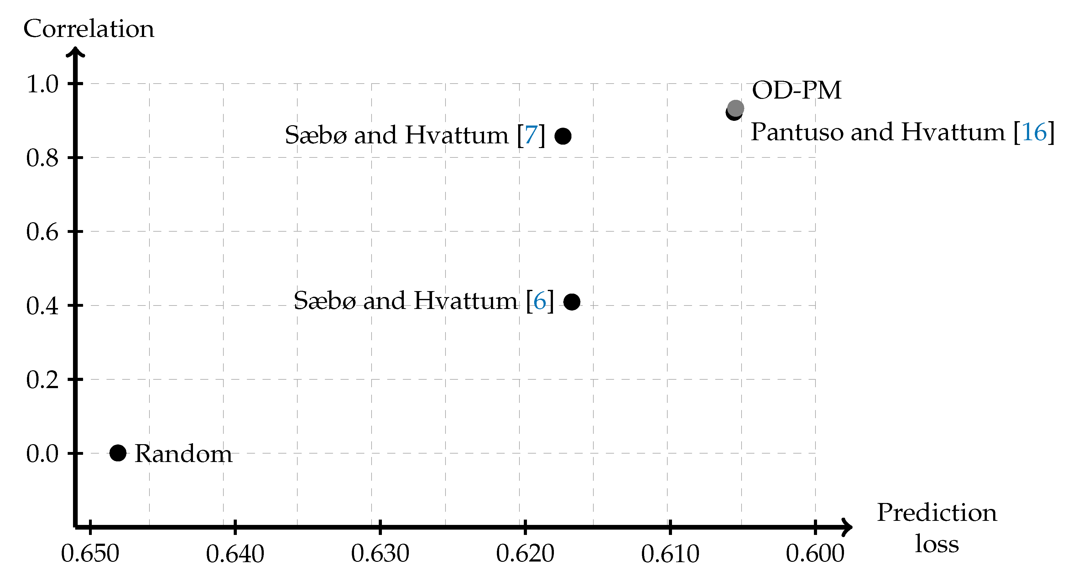
To provide benchmarks for the measures of validity and reliability, the new offensive–defensive plus–minus rating is compared to three previous plus–minus ratings, presented by Sbø and Hvattum [6], Sbø and Hvattum [7], and Pantuso and Hvattum [16]. An additional benchmark is the assignment of random ratings to each player. This provides the worst possible value of zero for the correlation coefficient. It also provides a bound on the prediction loss, where the only useful information for the prediction method consists of the historical distribution of match outcomes and the fact that one team has a home field advantage. Following this, an ablation study is also performed using the same metrics for evaluation, with the aim of analyzing the importance of several selected components of the new rating system.
To provide an analysis of the model parameters not directly related to the ratings of players, a bootstrapping technique is applied. Segments from the data set are sampled with replacement until reaching the same number of sampled segments as in the original data set. The rating model is then estimated based on the sampled segments, and the parameter values are recorded. This process is repeated 500 times, after which the values of each parameter are sorted, and the median value is output, together with the values that form a 95% confidence interval for the parameter.
Finally, the face validity of the ratings is assessed by calculating ratings on the whole data set and presenting the top ranked players and teams. In the ranking lists produced, a player must have played in at least one match in the data set during the last year up to July 2017 in order to be included. For the data set in question, this means that a total of 10,369 players are ranked. To rank teams, the players that have appeared for the team during the last year, and who have not played for any other teams since, are considered. Out of these, the 15 highest rated players are extracted for each team, and their average total rating is calculated as a measure of team strength.
5. Results
This section presents results from the tuning of hyperparameters, the testing of validity and reliability of the ratings, an ablation study, a bootstrap analysis of the estimated parameters of the rating model, and ranking lists for soccer players and teams.
5.1. Tuning of Hyperparameters
The values of the hyperparameters were initially set as those used by Pantuso and Hvattum [16], and then additional fine tuning was attempted. The latter did not result in significant changes, and the final values of the hyperparameters are , , , , , , and . The set of similar players is limited in size to , and players’ ages are confined by and . The main difference from the parameters used by Pantuso and Hvattum [16] is that is reduced from 16 to 12. In addition, is an additional regularization factor for age curves, whereas is an additional factor for the regularization of the difference in the offensive and defensive ratings of a player.
5.2. Validity and Reliability Testing
The validity and reliability measures for the new offensive–defensive plus–minus ratings are illustrated in Figure 3. It is clear that the new ratings (represented by a gray dot) perform almost exactly the same as the previous installment of plus–minus ratings by Pantuso and Hvattum [16] (represented by a black dot just below the new rating). This is perhaps explained by the fact that the regularization terms for the overall player ratings are very similar. In fact, the correlation coefficient between the final ratings calculated for the whole data set using either the new offensive–defensive ratings or the existing ratings from [16] is 0.99. This means that, effectively, the overall ratings are almost identical, and the only contribution from the new rating system is that the overall rating can be split into a defensive rating and an offensive rating.
5.3. Ablation Study
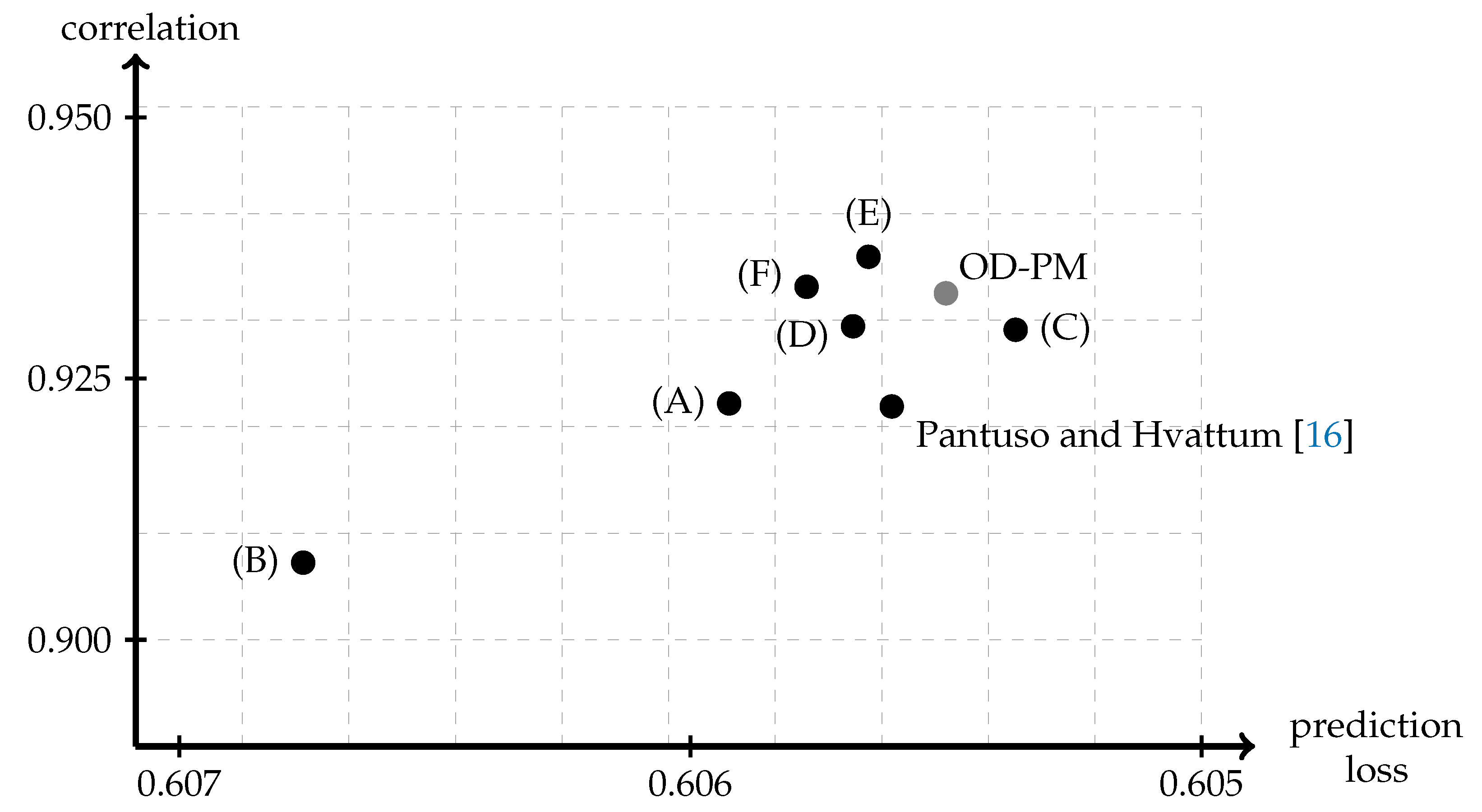
The new rating model has several components, and it is not immediately clear how each of them contributes to the rating system as a whole. To shed some light on this, an ablation study is conducted, where six different model variations are created by eliminating certain components from the full model. These model variations are then evaluated in the same framework as the full model, so that the importance of each eliminated component can be measured. The following variations of the model are considered:
- (A)
- Removing segment weights, that is, setting .
- (B)
- Removing the effect of player age, by setting .
- (C)
- Ignoring home field advantages, by setting .
- (D)
- Not considering red cards, by ignoring segments with missing players, i.e., removing all s from where for any n.
- (E)
- Removing the regularization terms for the difference between offensive and defensive ratings, by setting .
- (F)
- Not skipping offensive ratings for goal keepers, by enforcing and adjusting and by removing the exceptions for .
The results of the ablation study are illustrated in Figure 4, based on the validity and reliability of the resulting ratings. The differences between the model variations are very small, and the figure is only showing a small portion of the values for prediction loss and correlation given in Figure 3. The overall conclusion is that none of the model variations outperform the full model, but that the relative degradation in performance is small when modifying only a single model component. When ignoring home field advantages, the prediction loss of the method improves, but with a reduction in the reliability of ratings. On the other hand, when removing the additional regularization term for the difference between the offensive and defensive ratings of each player, the reliability increases at the expense of worse prediction loss values. However, in both of these cases, the deviations are very small.
5.4. Bootstrap Results
While the overall ratings produced from the new rating model is strongly correlated with the ratings produced by earlier versions of plus–minus ratings, it remains to be seen whether additional insights can be gained by splitting the overall rating into a defensive and an offensive component. To examine the effects of the coefficients of the model not directly related to the player ratings, a bootstrap procedure was applied, and its results are discussed in the following.
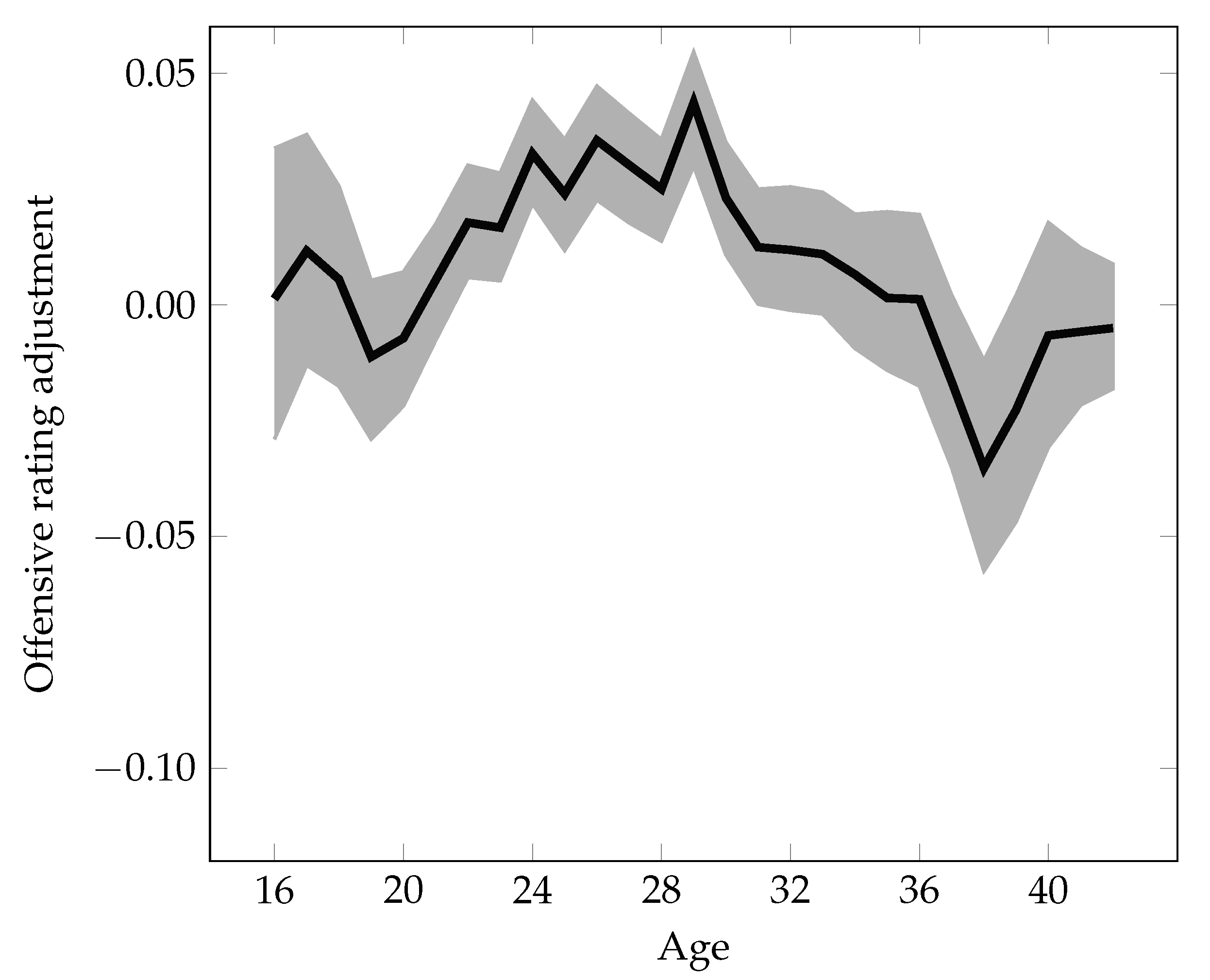
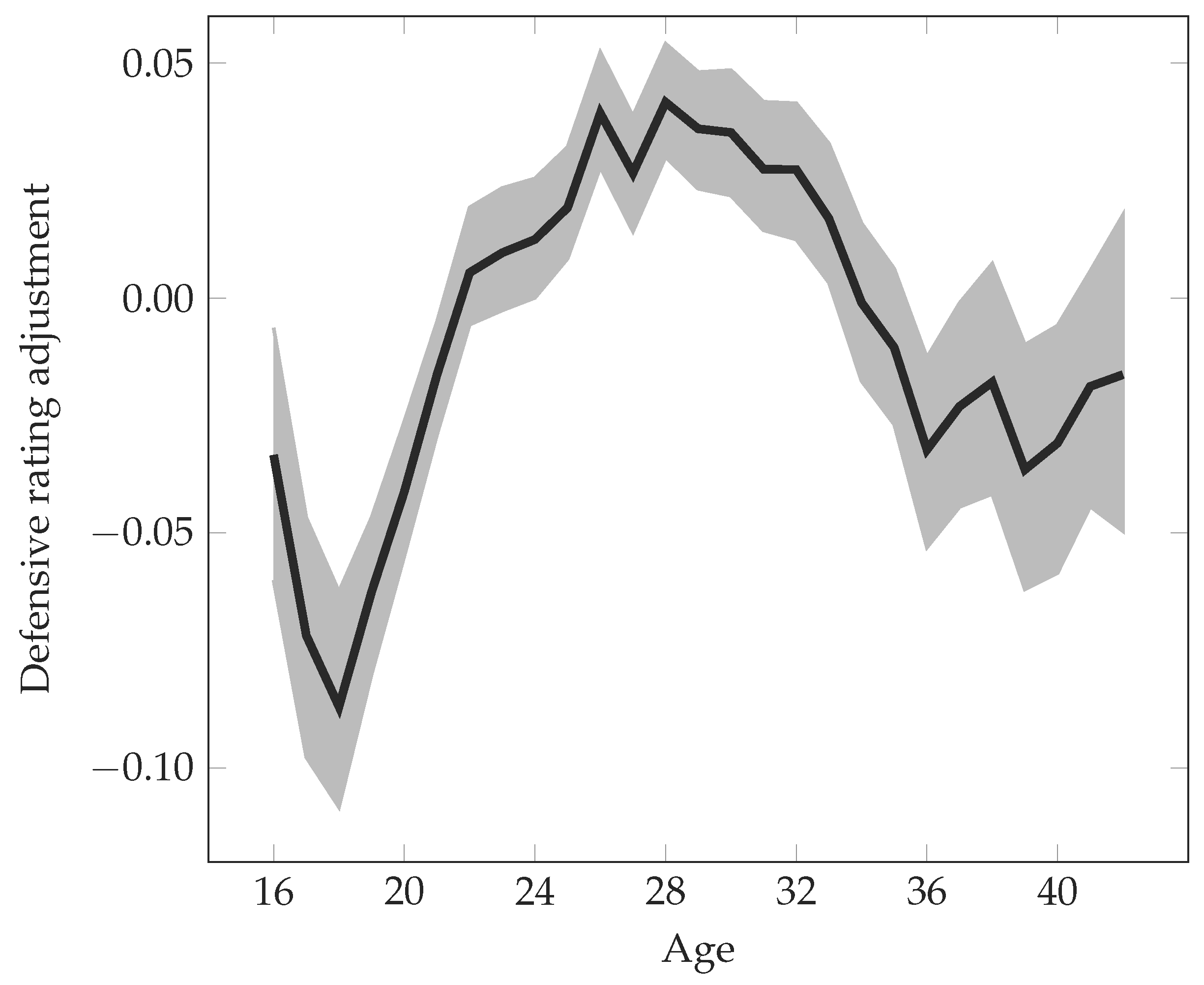
First, Figure 5 shows the effect of a player’s age on their offensive rating, whereas Figure 6 shows the effect of age on the defensive rating. There are few observations of players at the extreme ends of the age spectrum, so the regularization makes the age effects closer to zero for those. In general, the confidence intervals are narrower in the middle of the age range, which makes sense since there are more players in the data set with such ages, so the estimation is more reliable. The effect of age is much more pronounced for the defensive ratings, compared to the offensive ratings. In particular, younger players are relatively worse when it comes to defensive ratings. This could indicate that it is more important to use peak age players in defense, and less important to avoid young players up front.
Table 3 provides bootstrap estimates for the home field advantage parameters. The first observation is that overall, the home field advantage is in line with previous studies, for example Sbø and Hvattum [7] who found an overall advantage of 0.388 goals per 90 min for the home team. However, the offensive–defensive rating model uses the home field advantage to shift the baseline for goals scored by both teams—that is, the positive numbers for offensive advantages indicate that home teams score more goals than the baseline, whereas the negative numbers for defensive advantages indicate that away teams score more goals than the baseline.
The last column in Table 3 indicates the difference of the median in favor of the home team. This implies that certain leagues behave differently in terms of the total number of goals: While the overall home field advantage is similar for Italy and Portugal, with 0.33 goals in favor of the home team per 90 min, in Portugal, both teams score 0.27 goals more per 90 min than in Italy, all else being equal. Although the confidence intervals are wide, this is in line with the reputation that Italian football is defensively oriented. However, factors such as the distribution of playing strength between teams in a league may also contribute towards how the home field advantage is estimated by the model.
The overall home field advantage also seems to differ between competitions. It is highest for the UEFA Champions League (UCL) and Europa League (UEL), with 0.44 goals per 90 min. These competitions are special, since many of the rounds are played as two matches, one at home and one away, leading to the elimination of the overall losing team. The matches are also associated to longer travel distances than the domestic leagues, which may be another factor in explaining the larger home field advantage.
There could potentially be an additional change in the home field advantage when either team has players being sent off. However, the bootstrap estimation suggests that this change is very minor: when the home team has one player sent off, it scores 0.38 (with a 95% confidence interval [0.32, 0.44]) goals less and concedes 1.07 ([0.97, 1.18]) goals more per 90 min; on the other hand, when the away team has one player sent off, it scores 0.30 ([0.25, 0.36]) goals less and concedes 1.14 ([1.03, 1.22]) goals more per 90 min.
These estimates are also close to what was observed in previous studies in terms of their overall effect. For example, Sbø and Hvattum [7] found that a single red card was worth 1.53 goals per 90 min. They found, however, that additional dismissals were given a much smaller value, indicating that the first red card is more significant than the second red card to the same team. On this point the new model differs, indicating that, with a second red card for the home team, it scores 0.51 goals less and concedes 1.37 goals more per 90 min. Similarly, a second red card for the away team results in it scoring 0.27 goals less and conceding 1.55 goals more. Only for the third card to either team do the estimates become quite noisy, due to this being quite a rare event.
Table 4 shows bootstrap estimates for the league component of the player ratings. In general, these should provide an indication of the average quality of players in a given league. While these values only form a part of the rating of each player, they do contribute to the ratings of all players having appeared in the respective leagues. Even though the individual component of a player’s rating may contribute to shift the rating away from the league average, when taken across all players in a league, these individual differences may be expected to cancel out.
Some of the league component estimates seem to counter the effects of the home field advantage estimates. For example, the home field advantage in Italy indicates that relatively fewer goals are scored compared to other leagues, such as Portugal, as shown in Table 3. However, the league component of the player ratings indicate that the players in Italy contribute to both scoring and conceding more than players in Portugal. Although these two aspects seem to negate each other, it may also be that there is indeed a difference between how players contribute to scoring and conceding based on the league in which a match is played, and that this difference comes in addition to the innate abilities of the players appearing in the same league. In any case, the effect of the league components in the player ratings is much smaller than the effect of the home field advantage on the scoring rates.
Table 5 shows estimates for the parameter that is used in regularization of the difference between offensive and defensive ratings. Goalkeepers only have a defensive ratings, but for the other three positions, the parameters have the expected behavior, that is, defenders have, on average, a lower offensive rating than a defensive rating, and forwards have a higher offensive rating than defensive rating. For midfielders, the difference between the offensive and defensive ratings due to regularization is not significant.
In summary, the coefficients of the model not directly related to player ratings behave as expected, and can be used to identify how the age of players, the home field advantage, and players being sent off influences the outcome of a soccer match, both with respect to the number of goals scored and the number of goals conceded for each team. It is observed that, on average, players registered as defenders are relatively more important when it comes to reducing the number of goals conceded, whereas players registered as forwards are more important when it comes to increasing the number of goals scored.
5.5. Rankings
The final step of the evaluation of the new rating system is to look at the ratings produced and whether they are reasonable. To this end, lists of the top ten ranked players in different categories are presented below. In total 10,369 players are present in the full data set and have at least one appearance over the last year, and these are considered as eligible for the lists. Table 6 lists the players with the highest overall rating as of July 2017. Out of the 10,369 players, the model identifies Lionel Messi of Barcelona as having the highest overall rating. The other players at the top of the rating list are also well known players, and as for the model of [16], the new model does appear to identify playing strength in line with expectations.
At this point, though, it is more interesting to look at how the overall rating is split into offensive and defensive ratings. Of the players in the overall top 10, many have a high offensive rating and a lower defensive rating. As the number of goals scored by a team is non-negative, and since the model approximates this by taking the difference of offensive ratings of the scoring team and the defensive ratings of the conceding team, it is understandable that on average, offensive ratings are higher than defensive ratings. Considering all the 10,369 players, the average offensive rating is 0.091, while the average defensive rating is 0.014.
While the top list has players of different positions present, even the players in defensive positions have relatively high offensive ratings. It could be that the model does not successfully identify all defensive players as such, but it may also be that in some cases even defensive players contribute in a way that allows their teams to score more goals, rather than just to prevent goals from being conceded. Table 7, listing the ten players with highest offensive ratings, also includes some players that have appeared as defenders. The highest rated offensive player registered as a defender in the data set is Jerome Boateng of Bayern München, ranked as number 20 according to his offensive rating. While an aging Cristiano Ronaldo is still top three in terms of offensive rating, his age means that his defensive rating starts to drop (see Figure 6), and his overall rank is number 26.
Table 8 shows the highest rated players according to their defensive rating. As goalkeepers do not have any offensive rating, the model typically assigns them a high defensive rating, and the top list is dominated by goalkeepers. The first non-goalkeeper to appear on the list is Daniel Carvajal Ramos of Real Madrid at number 30, with a defensive rating of 0.188.
When looking at the top lists, it is apparent that the difference between offensive and defensive ratings is much larger for these players than the value indicated by the position difference in the regularization. Thus, the model is attempting to pick up whether each player’s contribution is mostly in terms of increasing the goals scored or reducing the goals conceded for the team. However, it is not clear from the top lists inspected whether the model is successfully doing so for all players.
Table 9 presents the top ten ranked teams, where the rank is determined based on the average overall rating for the 15 highest rated players in the squad. Player ratings are based on the full data set, representing the playing strength as of July 2017, and a player must have appeared at least once for the team in the last year to qualify for inclusion. While the following analysis considers the 15 highest rated players, selected to represent a starting line-up plus substitutes, the rankings of top teams typically do not change much if either reducing or increasing this number. The ratings illustrate that some teams are more defensively oriented than others. Real Madrid was the highest ranked team in July 2017. They had just won the UEFA Champions League twice in a row, and would go on to win again in the following season. The model suggests that they achieved this through having an effective attack, having a higher scoring ability than all other teams except Barcelona. Defensively, Real Madrid was less impressive, and the model ranks them as number 12 out of 316 club teams. The highest rated team in terms of defensive ratings is Atlético Madrid, with a defensive rating of 0.111, which corresponds well with how the team was perceived at the time.
The 15 highest ranked players of Bayern München are listed in Table 10. This table also indicates the peak ratings of each player, which are calculated based on the age effect curves as illustrated in Figure 5 and Figure 6. The three players with the highest peak ratings are Lewandowski, Robben, and Ribery. However, since the two latter are approaching the mid-30s, their current ratings are adjusted downwards accordingly. Some of the general impressions of the ratings in the list are reasonable: forwards tend to have lower defensive ratings, the defensive ratings of defenders are relatively high compared to their offensive ratings. However, there are some exceptions, such as the defender Boateng, who has a very high offensive rating, indicating that he is on the pitch when Bayern scores many of their goals. His defensive rating is not very high, indicating that his presence does not appear to prevent Bayern from conceding more goals than when other players take his place.
Finally, Table 11 lists all domestic leagues in the data set, sorted according to the average overall rating of the players with at least one appearance in the league during the 2016/2017 season. The ranking is similar to that indicated by the league component in Table 4. Among the minor differences, we see that the teams in ranks two to five have been scrambled, and that the Dutch Eredivisie is somewhat lower than indicated by the league component. While Table 9 showed that the best teams come from Spain and Germany, Table 11 shows that the top division of England has the best players on average.
6. Concluding Remarks
This paper provided a new plus–minus rating for individual players in soccer, where the contributions of the players are split into offensive and defensive contributions. The offensive rating indicates to what extent a player is contributing to the team scoring more goals, whereas the defensive rating indicates whether a player is contributing to the team conceding fewer goals.
Testing the ratings on a data set of more than 52 thousand matches, with more than 30 thousand unique players, demonstrates that it is feasible to split the plus–minus ratings into offensive and defensive ratings. Looking into the estimated parameters of the rating model, the split seems to make sense: defenders have higher defensive ratings and forwards have higher offensive ratings, compared to players of other positions. Furthermore, the age of a player influences offensive and defensive contributions differently, with defensive ratings being more sensitive to the player’s age. The home field advantage and the effect of player dismissals have an influence on both the number of goals scored and the number of goals conceded for the teams in a match. As an example, a red card has a negative effect both on the number of goals scored and conceded, but the effect on the number of goals conceded is stronger.
Although the new rating appears reasonable from an eagle eye perspective, when studying individual players, the ratings may be harder to reconcile with established opinion. As an example, a strong defender may be assigned a relatively low defensive rating and a high offensive rating. This could simply mean that the defender is more important to the team building up an attack, and comparably less important for the direct prevention of goals conceded. As such, offensive or defensive ratings that are in opposition to current perceptions of players can be useful triggers for discussions. However, it remains an open question as to whether the split in offensive and defensive ratings lead to a noisy and seemingly arbitrarily set defensive ratings, or whether the new ratings are able to detect patterns that are not common knowledge.
The reported experiments have some limitations. For one, they are based on a single data set, which, although large, may still be of insufficient size to calculate the best version of the offensive–defensive plus–minus ratings. In particular, it may be that additional seasons of data would lead to more stable results, and facilitate more robust settings for the hyperparameters of the rating model. In addition, there are few benchmarks to which the ratings can be compared. While this is true in general for overall player ratings, it is perhaps even more pronounced for defensive ratings. It may be that access to more granular data, such as event data, could facilitate improved defensive ratings.
In conclusion, the new ratings perform on par with previous ratings when it comes to predicting future match outcomes. The offensive–defensive ratings allow additional insights into the game, by assessing the importance of the home field advantage and red cards on the individual scoring rates of the teams.
For future research, generalizations of the model may be used to analyse additional elements, such as the effects of the playing schedule and player fatigue, or the effects of defensively or offensively oriented head coaches. The new rating model exploits information about player positions. It may be interesting to investigate whether more specific player position data could be used to improve the split into defensive and offensive ratings, for example, by taking into account the difference between center backs and full backs or wing backs.
Funding
This research received no external funding.
Acknowledgments
The author wishes to thank the three reviewers for their concrete and useful suggestions that helped to improve the manuscript.
Conflicts of Interest
The author declares no conflict of interest.
References
- Engelmann, J. Possession-based Player Performance Analysis in Basketball (Adjusted +/− and Related Concepts). In Handbook of Statistical Methods and Analyses in Sports; Albert, J., Glickmann, M., Swartz, T., Koning, R., Eds.; Chapman and Hall/CRC: Boca Raton, FL, USA, 2017; pp. 215–228. [Google Scholar]
- Hvattum, L. A comprehensive review of plus-minus ratings for evaluating individual players in team sports. Int. J. Comput. Sci. Sport 2019, 18, 1–23. [Google Scholar] [CrossRef] [Green Version]
- Winston, W. Mathletics; Princeton University Press: Princeton, NJ, USA, 2009. [Google Scholar]
- Sill, J. Improved NBA Adjusted +/− Using Regularization and Out-of-Sample Testing. In Proceedings of the 2010 MIT Sloan Sports Analytics Conference, Boston, MA, USA, 6 March 2010. [Google Scholar]
- Ehrlich, J.; Sanders, S.; Boudreaux, C. The relative wages of offense and defense in the NBA: A setting for win-maximization arbitrage? J. Quant. Anal. Sport 2019, 15, 213–224. [Google Scholar] [CrossRef]
- Sæbø, O.; Hvattum, L. Evaluating the Efficiency of the Association Football Transfer Market Using Regression Based Player Ratings. 2015 NIK: Norsk Informatikkonferanse. Available online: https://ojs.bibsys.no/index.php/NIK/article/view/246 (accessed on 30 September 2020).
- Sæbø, O.; Hvattum, L. Modelling the financial contribution of soccer players to their clubs. J. Sport. Anal. 2019, 5, 23–34. [Google Scholar] [CrossRef] [Green Version]
- Kharrat, T.; Peña, J.L.; McHale, I. Plus-minus player ratings for soccer. Eur. J. Oper. Res. 2020, 283, 726–736. [Google Scholar] [CrossRef] [Green Version]
- Bohrmann, F. Problems with an Adjusted Plus Minus Metric in Football. 2011. Available online: http://www.soccerstatistically.com/blog/2011/12/28/problems-with-an-adjusted-plus-minus-metric-in-football.html (accessed on 13 September 2018).
- Hamilton, H. Adjusted Plus/Minus in Football—Why It’s Hard, and Why It’s Probably Useless. 2014. Available online: http://www.soccermetrics.net/player-performance/adjusted-plus-minus-deep-analysis (accessed on 13 September 2018).
- Sittl, R.; Warnke, A. Competitive Balance and Assortative Matching in the German Bundesliga; Discussion Paper No. 16-058; ZEW Centre for European Economic Research: Mannheim, Germany, 2016. [Google Scholar]
- Vilain, J.B.; Kolkovsky, R. Estimating Individual Productivity in Football. 2016. Available online: http://econ.sciences-po.fr/sites/default/files/file/jbvilain.pdf (accessed on 3 August 2018).
- Schultze, S.; Wellbrock, C.M. A weighted plus/minus metric for individual soccer player performance. J. Sport. Anal. 2018, 4, 121–131. [Google Scholar] [CrossRef] [Green Version]
- Matano, F.; Richardson, L.; Pospisil, T.; Eubanks, C.; Qin, J. Augmenting adjusted plus-minus in soccer with FIFA ratings. arXiv 2018, arXiv:1810.08032v1. [Google Scholar]
- Volckaert, T. Evaluating the Accuracy of Players’ Market Values in the Belgian pro League Using Regression Based Player Ratings. Master’s Thesis, Ghent University, Ghent, Belgium, 2020. [Google Scholar]
- Pantuso, G.; Hvattum, L. Maximizing performance with an eye on the finances: A chance-constrained model for football transfer market decisions. arXiv 2019, arXiv:1911.04689. [Google Scholar]
- Gelade, G.; Hvattum, L. On the relationship between +/− ratings and event-level performance statistics. J. Sport. Anal. 2020, 6, 85–97. [Google Scholar] [CrossRef] [Green Version]
- Arntzen, H.; Hvattum, L. Predicting match outcomes in association football using team ratings and player ratings. Stat. Model. 2020. forthcoming. [Google Scholar] [CrossRef]
- Vilain, J.B. Three Essays in Applied Economics. Ph.D. Thesis, Sciences Po Paris, Paris, France, 2018. [Google Scholar]
- Rosenbaum, D. Defense Is All About Keeping the Other Team from Scoring. 2005. Available online: http://82games.com/rosenbaum3.htm (accessed on 28 September 2018).
- Witus, E. Offensive and Defensive Adjusted Plus/Minus. 2008. Available online: http://www.countthebasket.com:80/blog/2008/06/03/offensive-and-defensive-adjusted-plus-minus/ (accessed on 31 March 2009).
- Ilardi, S.; Barzilai, A. Adjusted Plus-Minus Ratings: New and Improved for 2007–2008. 2008. Available online: http://www.82games.com/ilardi2.htm (accessed on 31 August 2009).
- Fearnhead, P.; Taylor, B. On estimating the ability of NBA players. J. Quant. Anal. Sport. 2011, 7. [Google Scholar] [CrossRef] [Green Version]
- Kang, K. Estimation of NBA Players’ Offense/Defense Ratings through Shrinkage Estimation. Honors Thesis, Carnegie Mellon University, Pittsburgh, PA, USA, 2014. [Google Scholar] [CrossRef]
- Macdonald, B. A regression-based adjusted plus-minus statistic for NHL players. J. Quant. Anal. Sport. 2011, 7. [Google Scholar] [CrossRef] [Green Version]
- Macdonald, B. An Improved Adjusted Plus-Minus Statistic for NHL Players. In Proceedings of the MIT Sloan Sports Analytics Conference, Boston, MA, USA, 4–5 March 2011. [Google Scholar]
- Macdonald, B. Adjusted Plus-Minus for NHL Players using Ridge Regression with Goals, Shots, Fenwick, and Corsi. J. Quant. Anal. Sport. 2012, 8. [Google Scholar] [CrossRef] [Green Version]
- Macdonald, B. An Expected Goals Model for Evaluating NHL Teams and Players. In Proceedings of the 2012 MIT Sloan Sports Analytics Conference, Boston, MA, USA, 2–3 March 2012. [Google Scholar]
- Thomas, A.; Ventura, S.; Jensen, S.; Ma, S. Competing process hazard function models for player ratings in ice hockey. Ann. Appl. Stat. 2013, 7, 1497–1524. [Google Scholar] [CrossRef]
- Greene, W. Econometric Analysis, 7th ed.; Pearson: Harlow, UK, 2012. [Google Scholar]
- Witten, I.; Frank, E.; Hall, M. Data Mining: Practical Machine Learning Tools and Techniques; Morgan Kaufmann: Burlington, MA, USA, 2011. [Google Scholar]
- Constantinou, A.; Fenton, N. Solving the problem of inadequate scoring rules for assessing probabilistic football forecast models. J. Quant. Anal. Sport. 2012, 8. [Google Scholar] [CrossRef]
- Wheatcroft, E. Evaluating probabilistic forecasts of football matches: The case against ranked probability score. arXiv 2019, arXiv:1908.08980. [Google Scholar]
Figure 1.
Illustration of the parameters referring to the time of events.
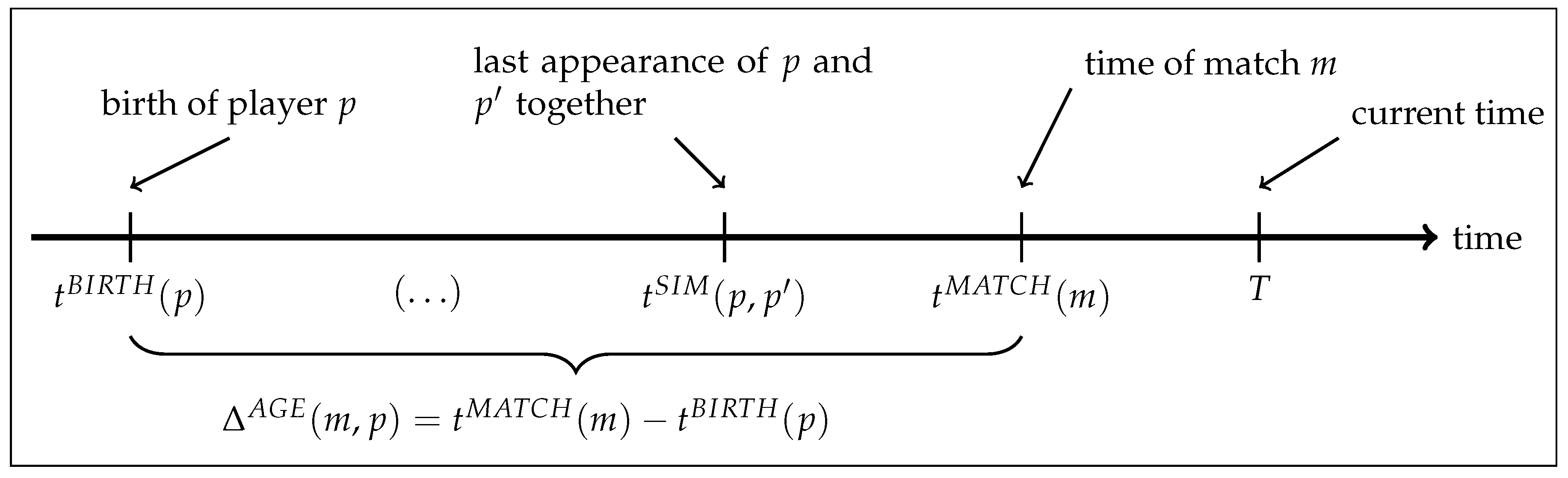
Figure 2.
Illustration of how the validity of ratings are evaluated based on the prediction loss, using a sliding window technique: the top showing the initial step where predictions are made, and the bottom showing the subsequent step.
Figure 2.
Illustration of how the validity of ratings are evaluated based on the prediction loss, using a sliding window technique: the top showing the initial step where predictions are made, and the bottom showing the subsequent step.
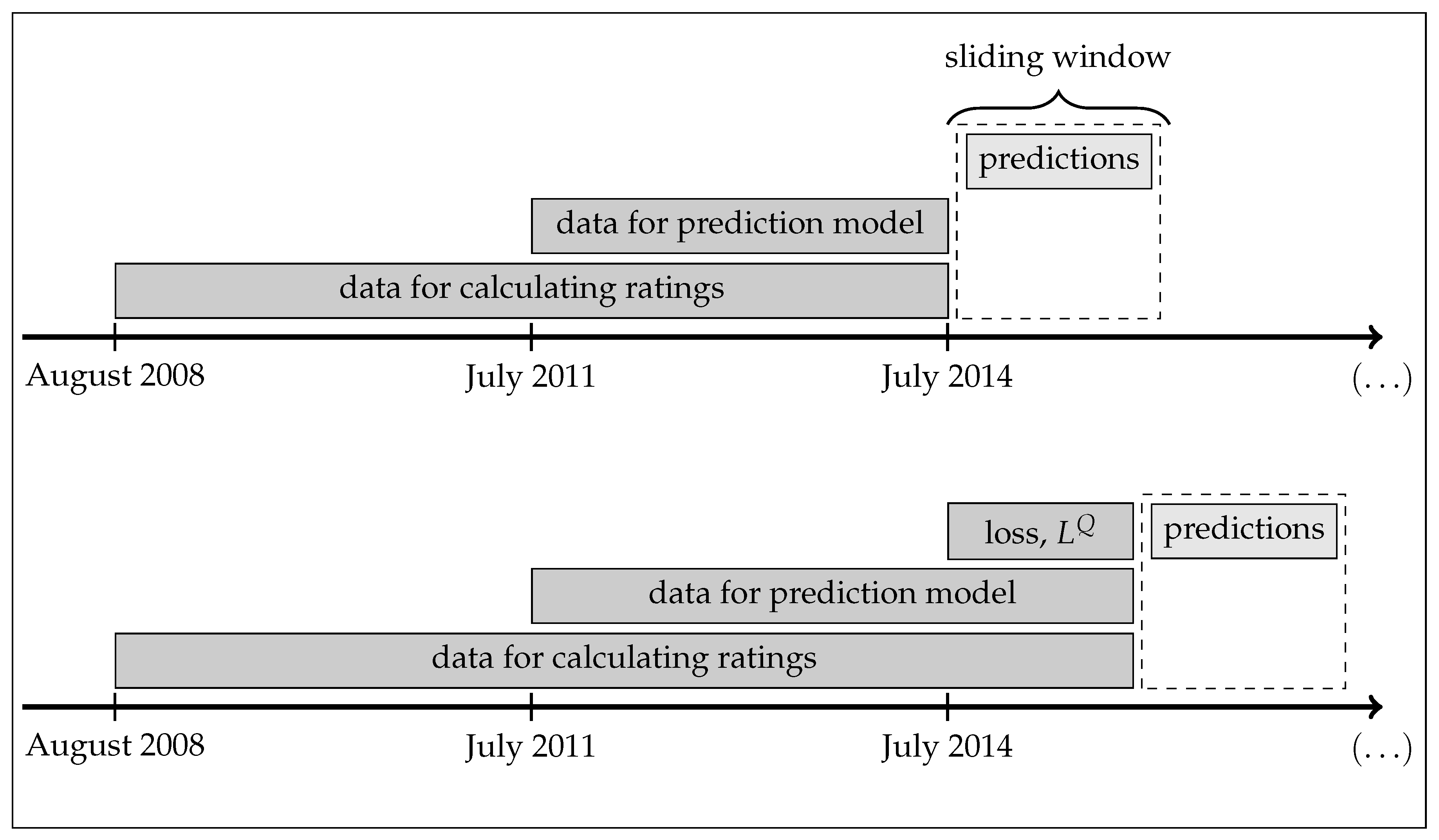
Figure 3.
Evaluation of rating methods based on reliability, measured as the correlation of ratings calculated on a data set randomly split in two halves, and validity, measured as the prediction loss for rating-based match outcome predictions.
Figure 3.
Evaluation of rating methods based on reliability, measured as the correlation of ratings calculated on a data set randomly split in two halves, and validity, measured as the prediction loss for rating-based match outcome predictions.

Figure 4.
Ablation study for the new rating system, with evaluation metrics as in Figure 3.
Figure 4.
Ablation study for the new rating system, with evaluation metrics as in Figure 3.

Figure 5.
Effect of age on offensive ratings, showing median effect (black line) and 95% confidence interval (gray area) from bootstrap tests.
Figure 5.
Effect of age on offensive ratings, showing median effect (black line) and 95% confidence interval (gray area) from bootstrap tests.

Figure 6.
Effect of age on defensive ratings, showing median effect (black line) and 95% confidence interval (gray area) from bootstrap tests.
Figure 6.
Effect of age on defensive ratings, showing median effect (black line) and 95% confidence interval (gray area) from bootstrap tests.


Table 1.
Coefficients for and in a selected segment, scaled by and , but not by segment weights w or segment duration .
Table 1.
Coefficients for and in a selected segment, scaled by and , but not by segment weights w or segment duration .
| Age | ||||
|---|---|---|---|---|
| 21 | −0.836 | 0.929 | ||
| 22 | −1.364 | 1.516 | ||
| 23 | 0.055 | −0.050 | ||
| 24 | 1.045 | −0.950 | ||
| 25 | −0.190 | 0.211 | ||
| 26 | 0.836 | −1.556 | 1.728 | −0.760 |
| 27 | 2.058 | −2.698 | 2.974 | −1.871 |
| 28 | 2.044 | −3.116 | 2.264 | −1.858 |
| 29 | 2.762 | −1.241 | 1.379 | −2.511 |
| 30 | ||||
| 31 | 0.766 | −0.697 | ||
| 32 | 1.434 | −1.537 | ||
| 33 | −0.767 | |||
Table 2.
Coefficients for and in a selected segment, scaled by and , but not by segment weights w or segment duration .
Table 2.
Coefficients for and in a selected segment, scaled by and , but not by segment weights w or segment duration .
| League | |||||
|---|---|---|---|---|---|
| Spain | Primera División | 8.617 | −7.700 | 7.944 | −8.167 |
| Spain | Segunda División | 0.550 | −3.300 | 3.056 | −0.833 |
| England | Premier League | 0.917 | −1.167 | ||
| Germany | Bundesliga | 0.550 | −0.500 | ||
| Netherlands | Eredivisie | 0.367 | −0.333 | ||
Table 3.
Bootstrap estimates of home field advantages. The positive numbers for offensive advantages indicate that home teams score more goals than the baseline, whereas the negative numbers for defensive advantages indicate that away teams score more goals than the baseline. The last column indicates the difference of the median in favor of the home team.
| Offensive | Defensive | ||||
|---|---|---|---|---|---|
| Median | 95% CI | Median | 95% CI | Sum | |
| UCL/UEL | 0.60 | [0.48, 0.70] | −0.15 | [−0.25, −0.04] | 0.44 |
| Spain | 0.65 | [0.50, 0.79] | −0.24 | [−0.38, −0.10] | 0.41 |
| Netherlands | 0.72 | [0.56, 0.87] | −0.35 | [−0.51, −0.18] | 0.37 |
| Italy | 0.46 | [0.32, 0.62] | −0.13 | [−0.27, 0.03] | 0.33 |
| Portugal | 0.73 | [0.58, 0.89] | −0.40 | [−0.55, −0.25] | 0.33 |
| Germany | 0.55 | [0.42, 0.68] | −0.24 | [−0.36, −0.12] | 0.31 |
| France | 0.57 | [0.41, 0.71] | −0.26 | [−0.41, −0.10] | 0.31 |
| WC/Euro | 0.55 | [0.42, 0.67] | −0.25 | [−0.37, −0.13] | 0.29 |
| England | 0.50 | [0.38, 0.61] | −0.23 | [−0.34, −0.10] | 0.27 |
Table 4.
Bootstrap estimates for the league component of the player ratings.
| Offensive | Defensive | |||||
|---|---|---|---|---|---|---|
| Median | 95% CI | Median | 95% CI | Sum | ||
| England | Premier League | 0.11 | [0.10, 0.13] | 0.01 | [0.00, 0.02] | 0.12 |
| Spain | Primera División | 0.08 | [0.07, 0.09] | 0.00 | [−0.01, 0.01] | 0.08 |
| France | Ligue 1 | 0.06 | [0.05, 0.08] | 0.01 | [0.00, 0.02] | 0.07 |
| Germany | Bundesliga | 0.08 | [0.07, 0.09] | −0.01 | [−0.02, 0.01] | 0.07 |
| Italy | Serie A | 0.07 | [0.05, 0.08] | −0.03 | [−0.05, −0.02] | 0.03 |
| Netherlands | Eredivisie | 0.05 | [0.04, 0.07] | −0.02 | [−0.03, −0.01] | 0.03 |
| England | Championship | 0.05 | [0.04, 0.06] | −0.03 | [−0.04, −0.02] | 0.02 |
| Germany | 2. Bundesliga | 0.04 | [0.03, 0.05] | −0.03 | [−0.04, −0.02] | 0.02 |
| Portugal | Primeira Liga | 0.03 | [0.02, 0.04] | −0.01 | [−0.03, −0.01] | 0.01 |
| Italy | Serie B | 0.04 | [0.02, 0.05] | −0.03 | [−0.04, −0.02] | 0.00 |
| France | Ligue 2 | 0.03 | [0.02, 0.04] | −0.03 | [−0.04, −0.02] | 0.00 |
| Spain | Segunda División | 0.03 | [0.02, 0.04] | −0.03 | [−0.04, −0.02] | 0.00 |
| England | League One | 0.03 | [0.02, 0.04] | −0.03 | [−0.05, −0.02] | 0.00 |
| England | League Two | 0.02 | [0.01, 0.03] | −0.06 | [−0.07, −0.05] | −0.04 |
Table 5.
Bootstrap estimates for the differences in offensive and defensive ratings for players of different positions.
Table 5.
Bootstrap estimates for the differences in offensive and defensive ratings for players of different positions.
| Difference | ||
|---|---|---|
| Position | Median | 95% CI |
| Goalkeeper | NA | NA |
| Defender | −0.05 | [−0.06, −0.04] |
| Midfielder | 0.00 | [−0.01, 0.01] |
| Forward | 0.07 | [0.05, 0.08] |
Table 6.
Top 10 rated players, estimated using the full data set from August 2008 to July 2017.
| Rank | Name | Nationality | Position | Age | Minutes | Offensive | Defensive | Total |
|---|---|---|---|---|---|---|---|---|
| 1 | Lionel Messi | Argentina | F | 30 | 31,132 | 0.382 | 0.015 | 0.397 |
| 2 | R. Lewandowski | Poland | F | 28 | 26,419 | 0.340 | 0.052 | 0.393 |
| 3 | Mesut Özil | Germany | M, F | 28 | 29,568 | 0.327 | 0.064 | 0.391 |
| 4 | Thiago Alcantara | Spain | M, F | 26 | 13,101 | 0.280 | 0.106 | 0.386 |
| 5 | Luis Suarez | Uruguay | F | 30 | 27,223 | 0.387 | −0.004 | 0.382 |
| 6 | Marcelo | Brazil | D, M | 29 | 24,966 | 0.323 | 0.058 | 0.382 |
| 7 | Sergio Busquets | Spain | D, M | 28 | 30,423 | 0.303 | 0.067 | 0.371 |
| 8 | David Alaba | Austria | D, M | 25 | 21,988 | 0.248 | 0.118 | 0.367 |
| 9 | Thomas Müller | Germany | F | 27 | 30,459 | 0.282 | 0.084 | 0.366 |
| 10 | T. Alderweireld | Belgium | D | 28 | 27,454 | 0.216 | 0.148 | 0.365 |
Table 7.
Top 10 players based on offensive ratings, estimated using the full data set from August 2008 to July 2017.
Table 7.
Top 10 players based on offensive ratings, estimated using the full data set from August 2008 to July 2017.
| Rank | Name | Nationality | Position | Age | Minutes | Offensive | Defensive | Total |
|---|---|---|---|---|---|---|---|---|
| 1 | Luis Suarez | Uruguay | F | 30 | 27,223 | 0.387 | −0.004 | 0.382 |
| 2 | Lionel Messi | Argentina | F | 30 | 31,132 | 0.382 | 0.015 | 0.397 |
| 3 | Cristiano Ronaldo | Portugal | F | 32 | 34,880 | 0.341 | −0.015 | 0.325 |
| 4 | R. Lewandowski | Poland | F | 28 | 26,419 | 0.340 | 0.052 | 0.393 |
| 5 | D. Sturridge | England | F | 27 | 12,901 | 0.333 | −0.007 | 0.325 |
| 6 | Mesut Özil | Germany | M, F | 28 | 29,568 | 0.327 | 0.064 | 0.391 |
| 7 | Marcelo | Brazil | D, M | 29 | 24,966 | 0.323 | 0.058 | 0.382 |
| 8 | J. Rodriguez | Colombia | M, F | 25 | 15,494 | 0.312 | 0.047 | 0.360 |
| 9 | Alvaro Morata | Spain | F | 24 | 8665 | 0.305 | 0.015 | 0.320 |
| 10 | Sergio Busquets | Spain | D, M | 28 | 30,423 | 0.303 | 0.067 | 0.371 |
Table 8.
Top 10 players based on defensive ratings, estimated using the full data set from August 2008 to July 2017.
Table 8.
Top 10 players based on defensive ratings, estimated using the full data set from August 2008 to July 2017.
| Rank | Name | Nationality | Position | Age | Minutes | Offensive | Defensive | Total |
|---|---|---|---|---|---|---|---|---|
| 1 | Manuel Neuer | Germany | G | 31 | 35,738 | NA | 0.300 | 0.300 |
| 2 | Thibaut Courtois | Belgium | G | 25 | 24,392 | NA | 0.284 | 0.284 |
| 3 | M.-A. ter Stegen | Germany | G | 25 | 17,301 | NA | 0.271 | 0.271 |
| 4 | Keylor Navas | Costa Rica | G | 30 | 17,128 | NA | 0.270 | 0.270 |
| 5 | Jan Oblak | Slovenia | G | 24 | 15,423 | NA | 0.253 | 0.253 |
| 6 | Roman Burki | Switzerland | G | 26 | 10,155 | NA | 0.251 | 0.251 |
| 7 | W. Szczesny | Poland | G | 27 | 25,620 | NA | 0.248 | 0.248 |
| 8 | Petr Cech | Czech | G | 35 | 33,171 | NA | 0.237 | 0.237 |
| 9 | Kevin Trapp | Germany | G | 26 | 17,620 | NA | 0.228 | 0.228 |
| 10 | Fraser Forster | England | G | 29 | 15,686 | NA | 0.227 | 0.227 |
Table 9.
Top 10 teams in July 2017 based on the average rating of the best 15 players of the team, estimated using the full data set from August 2008 to July 2017.
Table 9.
Top 10 teams in July 2017 based on the average rating of the best 15 players of the team, estimated using the full data set from August 2008 to July 2017.
| Rank | Team | League | Age | Offensive | Defensive | Total |
|---|---|---|---|---|---|---|
| 1 | Real Madrid | Spain | 27.5 | 0.250 | 0.080 | 0.331 |
| 2 | Bayern München | Germany | 29.2 | 0.232 | 0.105 | 0.322 |
| 3 | Barcelona | Spain | 27.3 | 0.253 | 0.075 | 0.311 |
| 4 | Borussia Dortmund | Germany | 27.4 | 0.205 | 0.085 | 0.277 |
| 5 | Chelsea | England | 27.6 | 0.196 | 0.091 | 0.275 |
| 6 | Juventus | Italy | 29.3 | 0.175 | 0.097 | 0.273 |
| 7 | Arsenal | England | 27.5 | 0.192 | 0.089 | 0.268 |
| 8 | Tottenham Hotspur | England | 26.1 | 0.184 | 0.094 | 0.265 |
| 9 | Manchester City | England | 29.4 | 0.194 | 0.070 | 0.264 |
| 10 | Manchester United | England | 27.8 | 0.159 | 0.102 | 0.262 |
Table 10.
Top 15 rated players of Bayern München in July 2017, estimated using the full data set from August 2008 to July 2017.
Table 10.
Top 15 rated players of Bayern München in July 2017, estimated using the full data set from August 2008 to July 2017.
| Offensive | Defensive | Total | |||||||
|---|---|---|---|---|---|---|---|---|---|
| Rank | Name | Position | Age | Current | Peak | Current | Peak | Current | Peak |
| 1 | R. Lewandowski | F | 28 | 0.340 | 0.349 | 0.052 | 0.065 | 0.393 | 0.410 |
| 2 | Thiago Alcantara | M | 26 | 0.280 | 0.286 | 0.106 | 0.108 | 0.386 | 0.390 |
| 3 | David Alaba | D, M | 25 | 0.248 | 0.260 | 0.118 | 0.134 | 0.367 | 0.389 |
| 4 | Thomas Muller | F | 27 | 0.282 | 0.302 | 0.084 | 0.091 | 0.366 | 0.389 |
| 5 | Jerome Boateng | D | 28 | 0.286 | 0.296 | 0.075 | 0.087 | 0.362 | 0.379 |
| 6 | Mats Hummels | D, M | 28 | 0.211 | 0.225 | 0.114 | 0.124 | 0.326 | 0.345 |
| 7 | Douglas Costa | M, F | 26 | 0.251 | 0.260 | 0.058 | 0.069 | 0.309 | 0.325 |
| 8 | Javi Martinez | D, M | 28 | 0.200 | 0.209 | 0.107 | 0.119 | 0.307 | 0.324 |
| 9 | Arjen Robben | F | 33 | 0.288 | 0.348 | 0.016 | 0.076 | 0.305 | 0.420 |
| 10 | Manuel Neuer | G | 31 | NA | NA | 0.300 | 0.330 | 0.300 | 0.330 |
| 11 | Philipp Lahm | D, M | 33 | 0.186 | 0.248 | 0.104 | 0.169 | 0.291 | 0.413 |
| 12 | Arturo Vidal | M | 30 | 0.121 | 0.153 | 0.165 | 0.185 | 0.286 | 0.334 |
| 13 | Juan Velasco | D, M, F | 24 | 0.162 | 0.166 | 0.120 | 0.139 | 0.283 | 0.301 |
| 14 | Rafinha | D, M | 31 | 0.134 | 0.180 | 0.143 | 0.175 | 0.277 | 0.351 |
| 15 | Franck Ribery | F | 34 | 0.257 | 0.323 | 0.011 | 0.087 | 0.268 | 0.406 |
Table 11.
List of domestic league competitions, sorted by average rating of players appearing in at least one match of the 2016/2017 season.
Table 11.
List of domestic league competitions, sorted by average rating of players appearing in at least one match of the 2016/2017 season.
| Rank | Country | Competition | Players | Offensive | Defensive | Total |
|---|---|---|---|---|---|---|
| 1 | England | Premier League | 524 | 0.138 | 0.049 | 0.177 |
| 2 | Germany | Bundesliga | 470 | 0.130 | 0.043 | 0.165 |
| 3 | Spain | Primera División | 541 | 0.123 | 0.043 | 0.156 |
| 4 | Italy | Serie A | 560 | 0.119 | 0.031 | 0.141 |
| 5 | France | Ligue 1 | 559 | 0.100 | 0.032 | 0.124 |
| 6 | England | Championship | 706 | 0.098 | 0.016 | 0.107 |
| 7 | Germany | 2. Bundesliga | 497 | 0.091 | 0.020 | 0.106 |
| 8 | Portugal | Primeira Liga | 523 | 0.076 | 0.025 | 0.095 |
| 9 | Spain | Segunda División | 614 | 0.079 | 0.021 | 0.094 |
| 10 | Netherlands | Eredivisie | 477 | 0.085 | 0.004 | 0.085 |
| 11 | Italy | Serie B | 641 | 0.076 | 0.013 | 0.082 |
| 12 | France | Ligue 2 | 528 | 0.074 | 0.009 | 0.077 |
| 13 | England | League One | 728 | 0.073 | −0.009 | 0.058 |
| 14 | England | League Two | 713 | 0.061 | −0.020 | 0.036 |
Publisher’s Note: MDPI stays neutral with regard to jurisdictional claims in published maps and institutional affiliations. |
© 2020 by the author. Licensee MDPI, Basel, Switzerland. This article is an open access article distributed under the terms and conditions of the Creative Commons Attribution (CC BY) license (http://creativecommons.org/licenses/by/4.0/).
Share and Cite
MDPI and ACS Style
Hvattum, L.M. Offensive and Defensive Plus–Minus Player Ratings for Soccer. Appl. Sci. 2020, 10, 7345. https://doi.org/10.3390/app10207345
AMA Style
Hvattum LM. Offensive and Defensive Plus–Minus Player Ratings for Soccer. Applied Sciences. 2020; 10(20):7345. https://doi.org/10.3390/app10207345
Chicago/Turabian StyleHvattum, Lars Magnus. 2020. "Offensive and Defensive Plus–Minus Player Ratings for Soccer" Applied Sciences 10, no. 20: 7345. https://doi.org/10.3390/app10207345
Note that from the first issue of 2016, this journal uses article numbers instead of page numbers. See further details here.