Article

A Review of Sample and Hold Systems and Design of a New Fractional Algorithm

by
Manuel Duarte Ortigueira
1 and
José Tenreiro Machado
2,*
1
CTS-UNINOVA and DEE of NOVA School of Science and Technology, Quinta da Torre, 2829-516 Caparica, Portugal
2
Department of Electrical Engineering, Institute of Engineering, Polytechnic of Porto, 4249-015 Porto, Portugal
*
Author to whom correspondence should be addressed.
Appl. Sci. 2020, 10(20), 7360; https://doi.org/10.3390/app10207360
Submission received: 3 October 2020 / Revised: 16 October 2020 / Accepted: 18 October 2020 / Published: 21 October 2020
(This article belongs to the Special Issue Control and Automation)

Abstract

:
Digital systems require sample and hold (S&H) systems to perform the conversion from analog to digital and vice versa. Besides the standard zero and first order holds, we find in the literature other versions, namely the fractional and exponential order holds, involving parameters that can be tuned to produce a superior performance. This paper reviews the fundamental concepts associated with the S&H and proposes a new fractional version. The systems are modeled both in the time and Laplace domains. The new S&H stemming from fractional calculus generalizes these devices. The different S&H systems are compared in the frequency domain and their relationships visualized by means of hierarchical clustering and multidimensional scaling representations. The novel strategy allows a better understanding of the possibilities and limitations of S&H systems.

1. Introduction

Fractional calculus (FC) generalizes the classical theory of differential calculus by including the concept of integrals and derivatives of real or complex order [1,2]. Many systems in physics and engineering can be generalized in the light of the FC concepts. However, a number of applications still remain to be fully explored under the light of FC. The areas of signal processing, dynamical systems and control has received considerable attention and the results show that the adoption of FC is clearly a fruitful research strategy [3,4,5,6].
Sample and hold (S&H) systems are commonly applied in mix analog/digital systems, being the standard procedure in discrete time systems to adopt zero-order holds (S&H-0) [7,8,9,10]. The devices, are simple to construct and ‘hold’ the signal sample during one time interval. They are a basic tool of the analog to digital (A/D) conversion. In the reverse operation (D/A) other types of S&H are used. For instance, the first-order hold (S&H-1) reconstructs signals as a piecewise linear approximations and may yield better fit at the price of a higher complexity. Other S&H are the fractional- and exponential- order holds, abbreviated as S&H- β and S&H-exp, with parameters 0 β 1 and τ > 0 , respectively, that also improve the technique at the cost of a slight additional complexity [11,12,13,14]. In fact, we can take advantage of the extra parameter β and τ by tuning their values for a particular application. Nonetheless, we observe the introduction of high frequency artifacts, that may pose difficulties in some applications. We can reduce this kind of distortion by using a modification of some of the above S&H systems. This change consists in introducing a delay of one sampling interval until a new sample appears. Therefore, instead of an extrapolation, as above, we are doing an interpolation [10,15]. Such procedures are very important in control [16,17] and telecommunications [9,18]. These topics are often neglected in practical applications. On one hand, the difference between theoretical and engineering implementations, due to physical restrictions, are overlooked. On the other hand, the possibilities for further improving the S&H systems, particularly when considering FC, remain to be explored.
This paper starts by reviewing the fundamental concepts associated with the S&H systems and proposes one generalization in the perspective of FC. The classical and fractional S&H are then compared based on their frequency responses. For that purpose we adopt the Euclidean and Canberra distances [19]. The distinct realizations of S&H are then represented using the Hierarchical Clustering (HC) and multidimensional scaling (MDS) computational tools [20,21,22,23]. Both schemes rely on constructing graphical representations of the items under study so that users can visualized their relationships. Items are ‘leafs’ of structures such as dendrogram or trees, for the HC, and as points in some abstract space, for the MDS. In both cases similar items are represented closely and vice-versa.
Bearing these ideas in mind the manuscript is organized as follows. Section 2 introduces the fundamental concepts concerning S&H. Section 3 discusses real-world implementations of S&H systems and proposes a fractional-order generalization. Section 4 analyses the transfer functions of the S&H systems under discussion. Finally, Section 5 outlines the conclusions.

2. Fundamental Concepts

With present day digital computer systems, and in areas such as signal processing and control, the conversion of an analog signal into a digital version requires sampling and quantisation. This action is called the A/D conversion (analog to digital conversion) and its inverse is the D/A conversion. In general, there are infinite continuous signals that can generate a given discrete signal. However, when the signals are bandlimited, meaning that they are of bounded support in the frequency domain, we can recover the original signal.
Definition 1.
The process of associating a discrete signal to a continuous one such that
1. 
the domain of the discrete signal is a discrete subset of the domain of the continuous signal,
2. 
the range of the discrete signal is also a discrete subset of the range of the continuous signal,
3. 
both signals, discrete and continuous, assume the same values at the intersection domains,
is named sampling [6].
The inverse operation, that is, the calculation of intermediate continuous values based on the discrete samples, is called interpolation or reconstruction. Ideally, the sampling operation is performed by the delta comb that we introduce in the follow-up.
Definition 2.
Let F and T = 1 F be two positive real constants. We define an almost linear time scale (ALTS) by [24]
t n = n · T + τ n , T = 1 / F , n Z ,
where τ n a zero mean sequence such that
0 | τ n | < T 4 .
The constant F is called sampling frequency, or density of the time scale, while its inverse T is the average graininess or sampling interval [25].
Remark 1.
In some applications, we prefer a half sampling interval delayed sequence t n = ( n + 1 / 2 ) · T + τ n .
Definition 3.
On the above ALTS (1) we define a uniform (in amplitude) almost periodic delta comb by
p ( t ) = n = + δ ( t t n ) , t R ,
that is considered as the ideal sampler, since its multiplication by any signal, y ( t ) , gives its sampled version
y p ( t ) = y ( t ) p ( t ) = n = + y ( t n ) δ ( t t n ) , t R .
This distribution has the Fourier transform (FT)
Y p ( ω ) = n = + y ( t n ) e j ω t n , ω R ,
where j = 1 and
Y p ( ω ) = y p ( t ) e j ω t d t .
Theorem 1.
Let Ω R + be the density of an odd ALTS, that is, so that ω n = ω n , given by ω n = n Ω + ν n , with ν n < Ω / 4 , n Z . The FT of the comb (3) in the time domain is another comb [24] in the frequency domain given by:
C ( ω ) = 2 π n = + C n δ ω ω n ,
where the coefficients,
C k = 1 T lim N 1 2 N + 1 n = N N e j ω k t n ,
form a bounded sequence and
Ω T 2 π = 1 .
This has as consequence that
Y p ( ω ) = n = + C n Y ( ω ω n ) ,
showing that Y p ( ω ) is an almost periodic function that results from the almost periodic repetition of Y ( ω ) . Therefore, if y ( t ) is not bandlimited, or if Ω is not high enough, then two consecutive repeated images of Y ( ω ) may overlap (phenomenon called aliasing) and it is not possible to recover the original signal by low-pass filtering. Unless something else is specified, we will assume that our signals are bandlimited in the follow-up. If the bandwidth is W, then we conclude that 2 W < Ω Ω / 4 < ω 1 . Otherwise, if we allow a spectral superposition, 2 W > ω 1 , then we cannot recover the original signal by low-pass filtering.
In the uniform sampling case t n = n T and ω n = n Ω , and we must have 2 W < Ω , stating the well known Nyquist rule: the sampling interval must be less than one half on the inverse of the higher frequency of the signal. The relation (7) shows that reducing the average distance between the impulses in the time domain (4) corresponds to increasing the distances between the replicas in the frequency domain (8).
Theorem 2.
Let x ( t ) be a continuous-time bandlimited signal with Fourier transform, X ( ω ) , that is null outside the band | ω | < W R + . We can recover x ( t ) from its samples x ( t n ) with a low-pass filtering provided that the filter frequency response is constant in the band of the signal. In the case of an ideal low-pass filter with bandwidth W, the output reads [24]
x ( t ) = n = x t n sin W t t n ( Ω / 2 ) t t n .
This theorem constitutes a generalization of the classical sampling theorem. This results deserves an interpretation in terms of linear systems. Let us consider that
g ( t ) = sin ( W t ) ( Ω / 2 ) t , t R ,
is the impulse response of a low-pass linear system and that the input to such system is
x p ( t ) = n = + x ( t n ) δ ( t t n ) .
Then the output will be given by the expression in (9). The signal g ( t ) is called the interpolating function and its FT is a rectangle which gives a justification to its name of ‘ideal low-pass filter’.
If the t n sequence is uniform, that is, if τ n 0 , then
x ( t ) = n = x ( n T ) sin W T t T n π t T n ,
that states the usual sampling theorem, where W T < π .

3. Sampling and Reconstruction

We reviewed the ideal sampling having as base the comb. In practice, we cannot implement the ideal Dirac impulses, but we can approximate them by narrow high rectangular pulses, r ( t ) , with area equal to 1. Nonetheless, we are interested in having the values x ( t n ) , rather than x ( t n ) δ ( t t n ) or its realistic version x ( t n ) r ( t t n ) . Therefore, we need to adopt a system that keeps, i.e. ‘memorizes’, the value x ( t n ) during a sufficient time for the computer system to be able to read the value.
The standard sampling is performed by a zero order hold. This scheme transforms the signal x ( t ) in a sequence of rectangles with height equal to x ( t n ) and width less or equal to the sampling interval. This procedure, called pulse amplitude modulation (usually abbreviated as PAM) in telecommunications [18], introduces an amplitude distortion and increases of the bandwidth that are corrected by a lowpass equalizer filter. However, there are several distinct ways of implementing the reconstruction and we review a few in the sequel.

3.1. The S&H Reconstruction by Extrapolation

Equation (9), is important from the mathematical point of view, but it is not of practical usefulness, since it requires the knowledge of all the signal values x ( t n ) , both at the past and future. This is a consequence of the fact that g ( t ) is not the impulse response of a causal system. To avoid such difficulty we use causal approximations generically called S&H systems. The most known are the zero- and one- order, but we can mention also the exponential hold. Let us analyze several approaches.

3.1.1. The Zero Order Sample and Hold

The output signal of a zero-order hold (S&H-0) has a zero slope between two consecutive sampling instants. Therefore, the S&H-0 circuit retains the measured value for a sampling instant at that level until the next sampling instant. The impulse response is a rectangle:
x ^ ( t ) = x ( t n ) u ( t t n ) u ( t t n + 1 ) ,
for t n t < t n + 1 , where u ( t ) is the Heaviside unit step.

3.1.2. The First-Order Sample and Hold

The first-order hold (S&H-1) exhibits an impulse response that has a constant slope between two consecutive sampling instants. This slope is the incremental ratio determined by the values of the two preceding samples. Thus, the first-order-hold predicts the response over the sampling interval from t n to t n + 1 as a ramp with the slope determined by the signal values at the two consecutive time instants. The impulse response is
x ^ ( t ) = x ( t n ) u ( t t n ) u ( t t n + 1 ) + ( t t n ) x ( t n ) x ( t n 1 ) t n t n 1 u ( t t n ) u ( t t n + 1 ) ,
for t n t < t n + 1 .

3.1.3. The Fractional-Order Sample and Hold

If we calculate the the arithmetic average between the S&H-0 and S&H-1, with weight factors 1 β and β , 0 β 1 , respectively, then we obtain the fractional-hold (S&H- β ) [12,13,14].
The impulse response of the S&H- β is:
x ^ ( t ) = x ( t n ) u ( t t n ) u ( t t n + 1 ) + β ( t t n ) x ( t n ) x ( t n 1 ) t n t n 1 u ( t t n ) u ( t t n + 1 ) ,
for t n t < t n + 1 . Therefore, we obtain the S&H-0 and S&H-1 for β = 0 and β = 1 , respectively.

3.1.4. The exponential order sample and hold

The exponential order hold S&H-exp is interesting because it has a simple electrical implementation based on an R C low-pass circuit [11]. The impulse response of the S&H-exp is:
x ^ ( t ) = x ( t n ) u ( t t n ) u ( t t n + 1 ) + 1 e ( t t n ) τ x ( t n ) x ( t n 1 ) t n t n 1 u ( t t n ) u ( t t n + 1 ) ,
for t n t < t n + 1 , where τ is the time constant. This expression is slightly different from the one presented in [11]. However, the previous expression is preferable because gives the S&H-0 when τ .

3.1.5. The α -Order Sample and Hold

Given the expressions for the S&H-0 and S&H-1 we can propose a generalization as follows.
Definition 4.
The α-order (S&H-α) is formulated as:
x ^ ( t ) = x ( t n ) + ( t t n ) α x ( t n ) x ( t n 1 ) t n t n 1 α ,
for t n t < t n + 1 , where α R + .
The impulse response is given by:
x ^ ( t ) = x ( t n ) u ( t t n ) u ( t t n + 1 ) + ( t t n ) α x ( t n ) x ( t n 1 ) t n t n 1 α u ( t t n ) u ( t t n + 1 ) ,
for t n t < t n + 1 .

3.2. The S&H Reconstruction by Interpolation

The S&H tools presented in the previous sub-section have a drawback, since they may lead to a discontinuous signal. The presence of discontinuities transforms the original bandlimited signal into fullband as we can observe in Figure 1. We can avoid this difficulty by implementing some kind of interpolation instead of having an extrapolation. However, this strategy has a price, since it involves the problem of a one sample delay. In many applications this delay has no visible effect. For example, in speech processing, with a sampling interval equal to 125 μ s , the effect of such delay is negligible. Nevertheless, not all the S&H techniques discussed above can be used. In fact, the S&H-0 leads always to discontinuities. The exponential hold has also that problem, unless we modify the parameter τ from sample to sample, which is not easily implementable. This problem does not happen with the proposed general S&H- α , where we only have to make a slight modification.
Definition 5.
The α-order (S&H-α) with delay is expressed as:
x ^ ( t ) = x ( t n ) + ( t t n ) α x ( t n + 1 ) x ( t n ) t n + 1 t n α , t n t t n + 1 .
The impulse response is given by:
x ^ ( t ) = x ( t n ) u ( t t n ) u ( t t n + 1 ) + ( t t n ) α x ( t n + 1 ) x ( t n ) t n + 1 t n α u ( t t n ) u ( t t n + 1 ) .
The S&H- α with delay (14) leads to a continuous signal, having as consequence that the amplitude spectrum decreases, at least, as fast as ω 2 when ω .
Example 1.
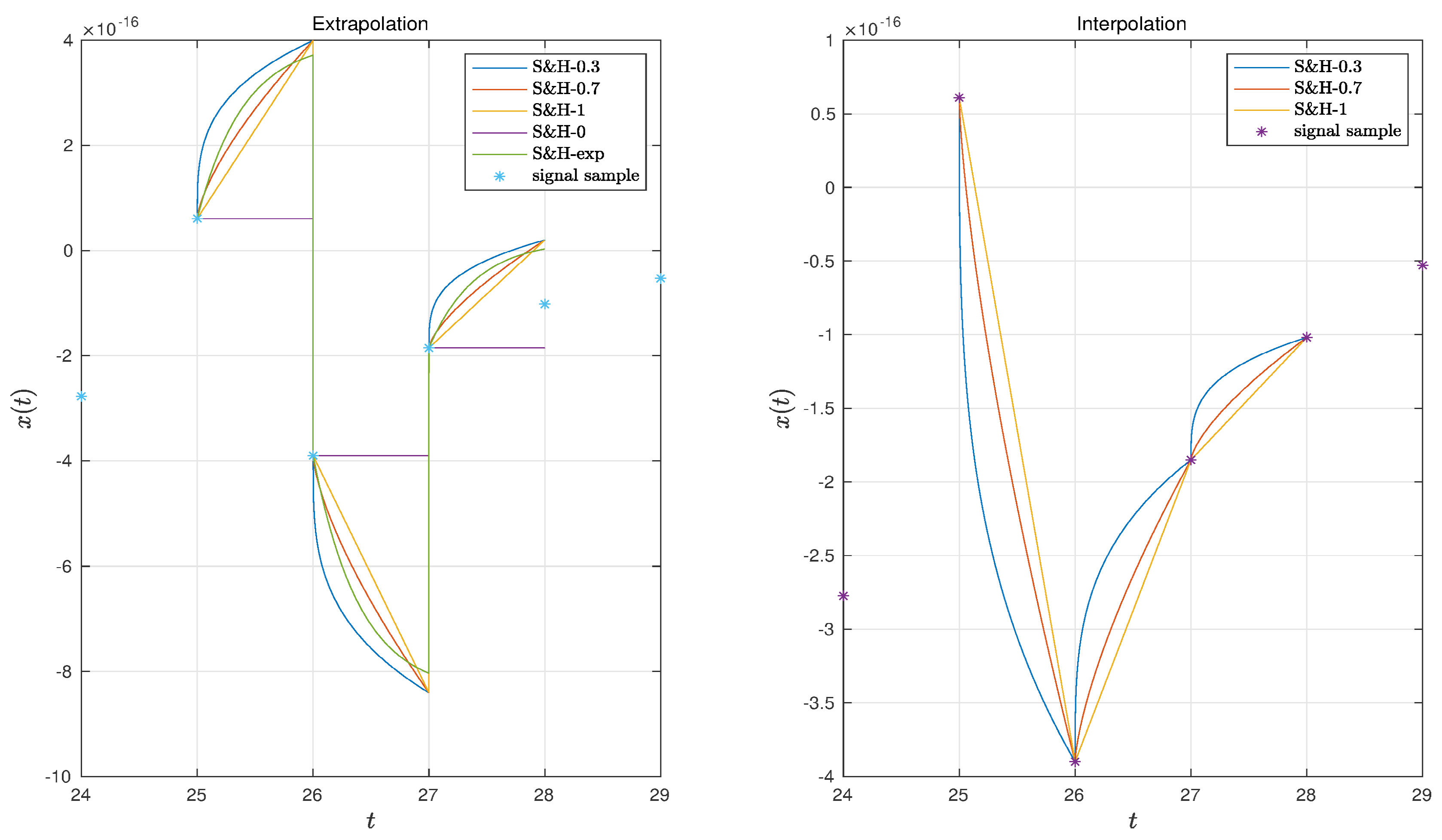
On the left of Figure 2 we depict the extrapolations obtained with the S&H-0, S&H-α (with α = 0.3 and α = 0.7 ), S&H-1 and S&H-exp (with τ = 200 ). On the right, we show the interpolations resulting from the S&H-α (with α = 0.3 and α = 0.7 ) and the S&H-1.
The difference between the two kinds of procedures is clear, as well as their distinct behavior.

4. The Transfer Functions of the S&H

In the previous section we introduced several S&H and presented the corresponding impulse responses. These have a general form
x ^ ( t ) = a r ( t ) + b g ( t ) ,
where a and b are real constants, r ( t ) = u ( t t n ) u ( t t n + 1 ) and g ( t ) is a short duration signal (i.e., a pulse). The first term in (16) is a rectangle and its Laplace transform is
L r ( t ) = e s t n e s t n + 1 s , s C ,
where L and s denote the Laplace operator and variable, respectively.
In the case of a uniform time scale, t n = n T ,
r ( t ) = u ( t n T ) u ( t ( n + 1 ) T ) ,
Equation (17) gives
L r ( t ) = e s n T e s ( n + 1 ) T s , s C .
The second term in (16) depends on the S&H method. For the fractional case (that includes α = 1 ), that is, for relations, (13) and (15), we obtain
L ( t t n ) α r ( t ) = e s t n 0 t n + 1 t n t α e s t d t , s C .
Let us introduce the lower incomplete gamma function defined as:
γ ( α , v ) = 0 v τ α 1 e τ d τ , α , v > 0 ,
that verifies the relation
γ ( α + 1 , v ) = α γ ( α , v ) v α e v .
We can write
0 t n + 1 t n t α e s t d t = α γ ( α , ( t n + 1 t n ) s ) s α + 1 t n + 1 t n s e ( t n + 1 t n ) s , R e ( s ) > 0 ,
that leads to
L ( t t n ) α r ( t ) = α γ ( α , ( t n + 1 t n ) s ) s α + 1 e s t n t n + 1 t n s e s t n + 1 , R e ( s ) > 0 .
For a uniform time scale Equation (20) yields
L ( t n T ) α r ( t ) = α γ ( α , T s ) s α + 1 e s n T T s e s ( n + 1 ) T , R e ( s ) > 0 .
In the particular case of α = 1 , we obtain γ ( 1 , v ) = 0 v e τ d τ = 1 e v , resulting
L ( t t n ) r ( t ) = e s t n e s t n + 1 s 2 t n + 1 t n s e s t n + 1 , R e ( s ) > 0 ,
and, therefore, to
L ( t n T ) r ( t ) = e s n T 1 e s T s 2 T s e s T , R e ( s ) > 0 .
Remark 2.
The choice of
g ( t ) = L 1 e s t n e s t n + 1 s α
is not of relevance, because it is not a function with finite support.
Let us recall the example discussed in the previous section. Figure 2 depicts the responses in the frequency domain.
We can compare the distinct items by means of the HC and MDS schemes. These clustering techniques allow the comparison and visualization of high dimensional data [26,27,28,29], such as in the case of controlling nonlinear systems [30].
In our case, the i-th item corresponds to the response in the frequency domain, G i f , that is represented by a numerical array of m points. A set of N items is then compared by means of suitable distances [31]. We adopt the Euclidean and Canberra distances given by:
d i j E = n = 1 m G i f G j f 2 ,
d i j C = n = 1 m G i f G j f G i f + G j f ,
where i , j = 1 , , N , so that N denotes the total number of items under comparison.
The first distance, d E , follows the standard logic of Euclidean spaces, while the second, d C , distinguishes more clearly values close to zero and in general is more robust to data sets including large and small values. The MDS computational recursive algorithm requires the input of a matrix of all item-to-item distances (i.e., a N dimensional square and symmetric matrix with main diagonal of zeros) and tries to reproduce approximately that matrix by mean a plot in a m M D S < m dimensional space where items consist of points. Therefore, similar items lead to close points and, inversely, very different items produce points very far apart. Usually, the dimensions m M D S = 2 or m M D S = 3 are used, because they allow a straightforward visualization [32,33].
In our case, the N = 9 items consist of the frequency responses G f described numerically in n f = 10 4 sample frequencies. The frequency responses characterize the original signal as well as the S&H-0, S&H- α (with α = 0.3 and α = 0.7 ), S&H-1 and S&H-exp (with τ = 200 ) and interpolations with S&H- α (with α = 0.3 and α = 0.7 ) and the S&H-1.
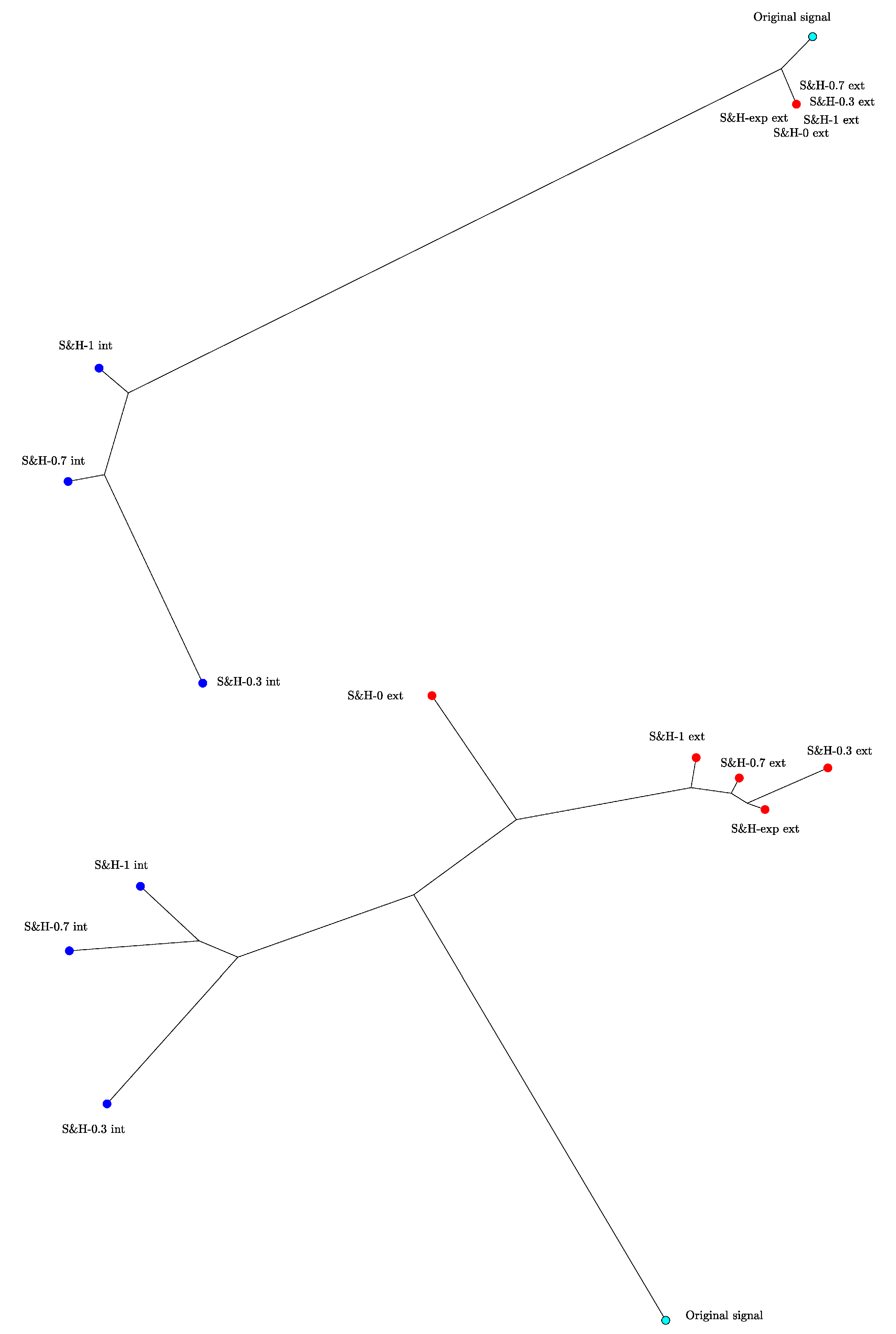
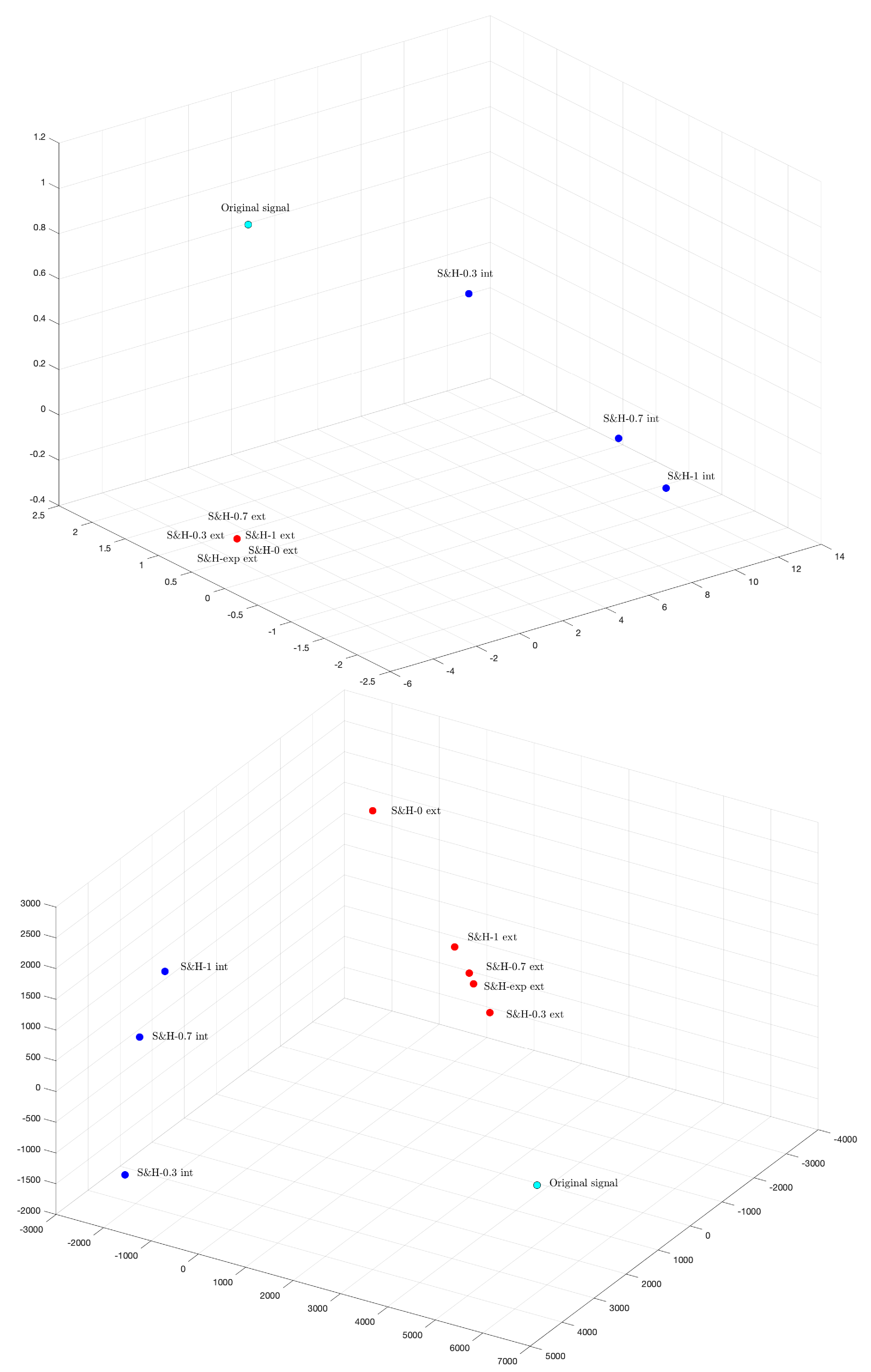
Figure 3 and Figure 4 show the HC tree and 3-dimensional MDS plots, respectively, when we compare the the frequency response of the extrapolations of the S&H-0, S&H- α (with α = 0.3 and α = 0.7 ), S&H-1 and S&H-exp (with τ = 200 ) and interpolations with S&H- α (with α = 0.3 and α = 0.7 ) and the S&H-1, using the Euclidean and Canberra distances.
We verify that extrapolations and interpolations (marked in red and blue, respectively) produce two distinct clusters. The extrapolation cluster is more concentrated than the interpolation, showing the behavioral in practical applications is almost independent of the adopted method, because they introduce similar discontinuities. However, in the interpolation case we see clearly an improvement when varying the parameter α .
This paper has not addressed the electronic implementation of such devices (interested readers can refer to [34,35,36,37,38,39,40] and references therein). Therefore, an open issue is the design of hardware systems capable of S&H advanced systems. Studies on the use of S&H- β in control systems report relevant results for improving the overall performance [41,42,43,44,45,46]. In this perspective, the construction of low cost general S&H may be a valuable option for obtaining equipment more friendly to the environment while not posing significant financial requirements.

5. Conclusions

S&H systems are a fundamental part of present-day digital systems. In spite of their widespread use, often their characteristic are neglected and, therefore, the possibility of improving the overall performance by using advanced S&H devices is not taken into account when designing signal discrete-time processing or control systems. This paper reviewed the main mathematical ideas associated with S&H systems. The main types of S&H systems were analyzed both in the time and Laplace domains. A generalization of S&H in the viewpoint of FC was formulated so that the additional degree of freedom provided by the fractional order can be tuned for each particular application. This strategy allows designers to take advantage of a more advanced system for improving the performance of systems posing considerable dynamical challenges and requiring that all sub-system are fully optimized. Furthermore, the HC and MDS clustering techniques were used to better verify the S&H characteristics. These tools allow a novel viewpoint for the quantitative comparison between multidimensional data sets. In particular, they can be applied also for improving the real-time performance of complex control systems.

Author Contributions

These two authors contribute equally to this paper. All authors have read and agreed to the published version of the manuscript.

Funding

This work was partially funded by National Funds through the Foundation for Science and Technology of Portugal, under the projects UIDB/00066/2020.

Conflicts of Interest

The authors declare no conflict of interest.

Abbreviations

The following abbreviations are used in this manuscript:
BLTbilateral Laplace transform
FTFourier transform
HCHierarchical clustering
LTLaplace transform
MDSMultidimensional scaling
S&HSample and hold
S&H-0Zero order sample and hold
S&H-1First-order sample and hold
S&H- β Fractional-order sample and hold
S&H-expExponential order sample and hold
S&H- α α -order sample and hold

References

  1. Ortigueira, M.D. Fractional Calculus for Scientists and Engineers; Lecture Notes in Electrical Engineering; Springer: Berlin/Heidelberg, Germany, 2011. [Google Scholar] [CrossRef]
  2. Machado, J.A.T.; Mainardi, F.; Kiryakova, V. Fractional calculus: Quo vadimus? (where are we going?). Fract. Calc. Appl. Anal. 2015, 18, 495–526. [Google Scholar] [CrossRef]
  3. Ortigueira, M.D. An Introduction to the Fractional Continuous-Time Linear Systems: The 21(st) Century Systems. IEEE Circuits Syst. Mag. 2008, 8, 19–26. [Google Scholar] [CrossRef] [Green Version]
  4. Ortigueira, M.D.; Machado, J.T. Fractional derivatives: The perspective of system theory. Mathematics 2019, 7, 150. [Google Scholar] [CrossRef] [Green Version]
  5. Valério, D.; da Costa, J.S. An Introduction to Fractional Control; Control Engineering; IET: London, UK, 2012. [Google Scholar]
  6. Ortigueira, M.D.; Valério, D. Fractional Signals and Systems; De Gruyter: Berlin, Germany; Boston, MA, USA, 2020. [Google Scholar] [CrossRef]
  7. Oppenheim, A.V.; Willsky, A.S.; Hamid, S. Signals and Systems, 2nd ed.; Prentice-Hall: Upper Saddle River, NJ, USA, 1997. [Google Scholar]
  8. Garrido, A.J.; De la Sen, M.; Bárcena, R. Approximate models to describe real sampling and hold processes based on multirate sampling techniques. In Proceedings of the American Control Conference, Chicago, IL, USA, 28–30 June 2000; Volume 1, pp. 195–199. [Google Scholar] [CrossRef]
  9. Kester, W. The Data Conversion Handbook. 2005. Available online: http://www.analog.com/library/analogdialogue/archives/39-06/data_conversion_handbook.html (accessed on 30 September 2020).
  10. Proakis, J.G.; Manolakis, D.G. Digital Signal Processing: Principles, Algorithms, and Applications; Prentice Hall: Upper Saddle River, NJ, USA, 2007. [Google Scholar]
  11. Pichler, H.; Pavuza, F.G.; Sommer, T. The exponential-hold circuit, properties and applications. In Proceedings of the 1993 IEEE Instrumentation and Measurement Technology Conference, Irvine, CA, USA, 18–20 May 1993; pp. 745–750. [Google Scholar] [CrossRef]
  12. Sheen, I.E.; Tsai, J.S.H.; Shieh, L.S. Optimal digital redesign of continuous-time systems using fractional-order hold. Optim. Control Appl. Meth. 1997, 18, 399–422. [Google Scholar] [CrossRef]
  13. Barcena, R.; de la Sen, M.; Sagastabeitia, I. Improving the stability properties of the zeros of sampled systems with fractional order hold. IEE Proc. Control Theory Appl. 2000, 147, 456–464. [Google Scholar] [CrossRef]
  14. Machado, J.A.T. Fractional order modelling of fractional-order holds. Nonlinear Dyn. 2012, 70, 789–796. [Google Scholar] [CrossRef] [Green Version]
  15. Bernhardsson, B. The predictive first order hold circuit. In Proceedings of the 29th IEEE Conference on Decision and Control, Honolulu, HI, USA, 5–7 December 1990; IEEE: Piscataway, NJ, USA, 1990. [Google Scholar]
  16. de Carvalho, J.L.M. Dynamical Systems and Automatic Control; Prentice Hall: Hertfordshire, UK, 1993. [Google Scholar]
  17. Dorf, R.C.; Bishop, R.H. Modern Control Systems; Pearson: London, UK, 2011. [Google Scholar]
  18. Haykin, S. Communication Systems; John Wiley & Sons: Hoboken, NJ, USA, 2008. [Google Scholar]
  19. Cha, S.-H. Comprehensive Survey on Distance/Similarity Measures between Probability Density Functions. Int. J. Math. Model. Methods Appl. Sci. 2007, 1, 300–307. [Google Scholar]
  20. Torgerson, W.S. Theory and Methods of Scaling; Wiley: New York, NY, USA, 1958. [Google Scholar]
  21. Sammo, J. A nonlinear mapping for data structure analysis. IEEE Trans. Comput. 1969, 18, 401–409. [Google Scholar] [CrossRef]
  22. Kruskal, J. Multidimensional Scaling; Sage Publications: Newbury Park, CA, USA, 1978. [Google Scholar]
  23. Kaufman, L.; Rousseeuw, P.J. Clustering Algorithms; Wiley-Interscience: Hoboken, NJ, USA, 2005. [Google Scholar]
  24. Ortigueira, M.D. The comb signal and its Fourier transform. Signal Process. 2001, 81, 581–592. [Google Scholar] [CrossRef] [Green Version]
  25. Ortigueira, M.D.; Torres, D.F.M.; Trujillo, J.J. Exponentials and Laplace transforms on nonuniform time scales. Commun. Nonlinear Sci. Numer. Simul. 2016, 39, 252–270. [Google Scholar] [CrossRef] [Green Version]
  26. Hartigan, J.A. Clustering Algorithms; John Wiley & Sons: New York, NY, USA, 1975. [Google Scholar]
  27. Shepard, R.N. The analysis of proximities: Multidimensional scaling with an unknown distance function. Psychometrika 1962, 27, 125–140. [Google Scholar] [CrossRef]
  28. Kruskal, J. Multidimensional scaling by optimizing goodness of fit to a nonmetric hypothesis. Psychometrika 1964, 29, 1–27. [Google Scholar] [CrossRef]
  29. Székely, G.J.; Rizzo, M.L. Hierarchical Clustering via Joint Between-Within Distances: Extending Ward’s Minimum Variance Method. J. Classif. 2005, 22, 151–183. [Google Scholar] [CrossRef]
  30. Machado, J.A.T. Visualizing Non-Linear Control System Performance by Means of Multidimensional Scaling. ASME Comput. Nonlinear Dyn. 2013, 8, 041017. [Google Scholar] [CrossRef] [Green Version]
  31. Deza, M.M.; Deza, E. Encyclopedia of Distances; Springer: Berlin/Heidelberg, Germany, 2009. [Google Scholar]
  32. Machado, J.A.T.; Lopes, A.M. Multidimensional Scaling Locus of Memristor and Fractional Elements. J. Adv. Res. 2020, 25, 147–157. [Google Scholar] [CrossRef] [PubMed]
  33. Machado, J.A.T.; Lopes, A.M. newblock Multidimensional Scaling and Visualization of Patterns in Prime Numbers. Commun. Nonlinear Sci. Numer. Simul. 2020, 83, 105128. [Google Scholar] [CrossRef]
  34. Marvasti, F. A new method to compensate for the sample-and-hold distortion. IEEE Trans. Acoust. Speech Signal Process. 1985, 33, 738–741. [Google Scholar] [CrossRef]
  35. Wang, Z. The fastest sample-and-hold circuit. Microelectron. J. 1990, 21, 49–52. [Google Scholar] [CrossRef]
  36. Van De Plassche, R. Sample-and-hold amplifiers. In Integrated Analog-To-Digital and Digital-To-Analog Converters; Springer: Boston, MA, USA, 1994; p. 264. [Google Scholar] [CrossRef]
  37. Taylor, H.R. Sample and hold circuits. In Data Acquisition for Sensor Systems; Springer: Boston, MA, USA, 1997. [Google Scholar] [CrossRef]
  38. Abolhasani, A.; Tohidi, M.; Hadidi, K.; Khoei, A. A new high-speed, high-resolution open-loop CMOS sample and hold. Analog. Integr. Circuits Signal Process. 2014, 78, 409–419. [Google Scholar] [CrossRef]
  39. Psychalinos, C.; Elwakil, A.; Maundy, B.; Allagui, A. Analysis and realization of a switched fractional-order-capacitor integrator. Int. J. Circuit Theory Appl. 2016, 44, 2035–2040. [Google Scholar] [CrossRef]
  40. Pelgrom, M. Analog-to-Digital Conversion; Springer: Cham, Switzerland, 2017. [Google Scholar]
  41. Yuz, J.I.; Goodwin, G.C.; Garnier, H. Generalised hold functions for fast sampling rates. In Proceedings of the 43rd IEEE Conference on Decision and Control, Atlantis, Bahamas, 14–17 December 2004; Volume 2, pp. 908–1913. [Google Scholar] [CrossRef]
  42. Trivedi, R. Low Power and High Speed Sample-and-Hold Circuit. In Proceedings of the 2006 49th IEEE International Midwest Symposium on Circuits and Systems, San Juan, PR, USA, 6–9 August 2006; pp. 453–456. [Google Scholar] [CrossRef]
  43. De la Sen, M. About Optimal Fractional Hold Circuits for Inter-sample Output Reconstruction in Sampled-data Systems. Sensors 2007, 7, 3146–3155. [Google Scholar] [CrossRef] [PubMed] [Green Version]
  44. Nishi, M.; Ishitobi, M. Sampled-Data Models for Nonlinear Systems with a Fractional-Order Hold. In Proceedings of the 18th IEEE International Conference on Control Applications Part of 2009 IEEE Multi-Conference on Systems and Control, Saint Petersburg, Russia, 8–10 July 2009; pp. 153–158. [Google Scholar] [CrossRef]
  45. Nishi, M.; Ishitobi, M. Sampled-data models for affine nonlinear systems using a fractional-order hold and their zero dynamics. Artif. Life Robot. 2010, 15, 500–503. [Google Scholar] [CrossRef]
  46. Zeng, C.; Xiang, S.; He, Y.; Ding, Q. Nonlinear Sampled-Data Systems with a Generalized Hold Polynomial-Function for Fast Sampling Rates. J. Syst. Sci. Complex. 2019, 32, 1572–1596. [Google Scholar] [CrossRef]
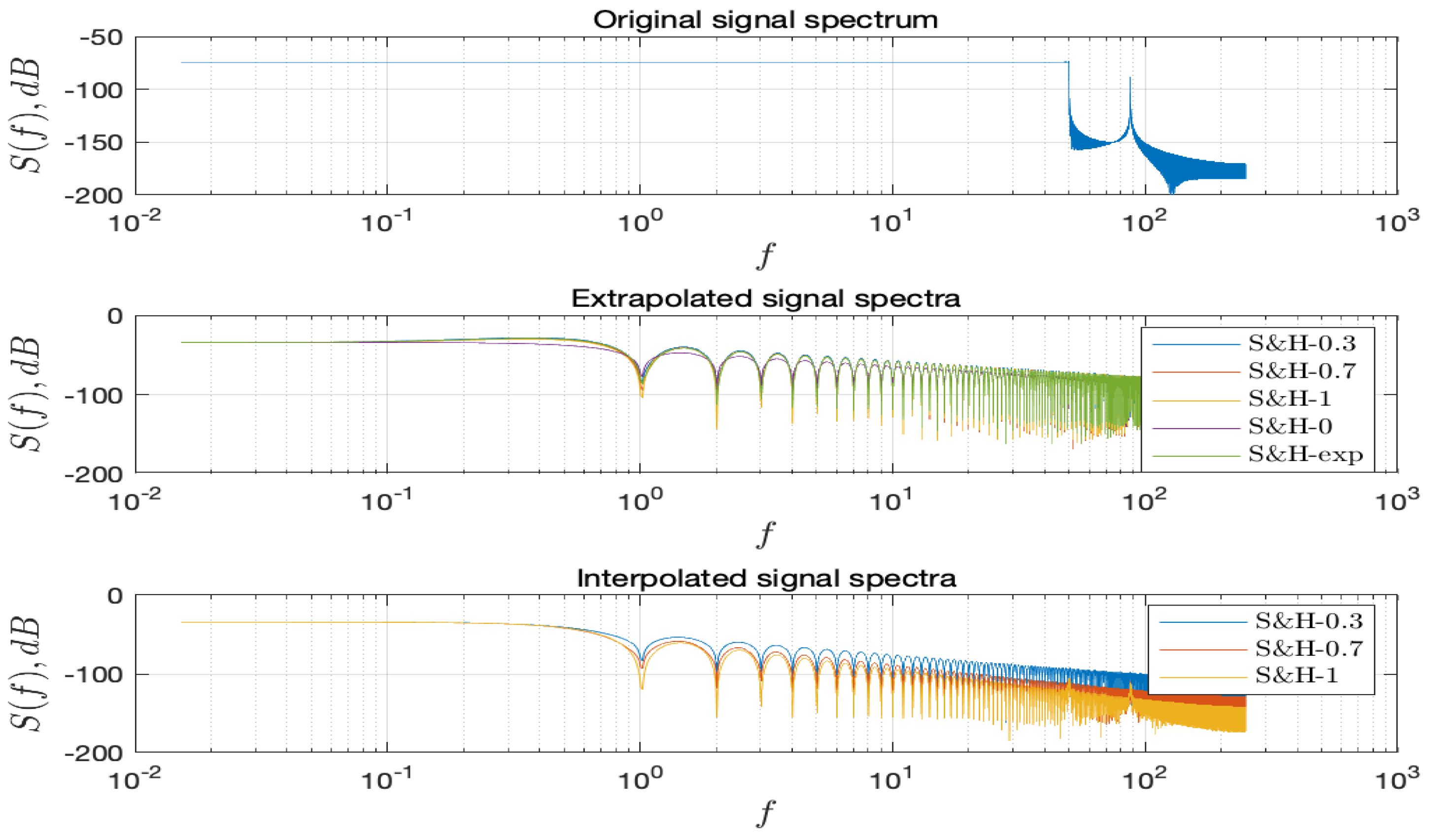
Figure 1. Frequency response of the extrapolations of the S&H-0, S&H- α (with α = 0.3 and α = 0.7 ), S&H-1 and S&H-exp (with τ = 200 ) and interpolations with S&H- α (with α = 0.3 and α = 0.7 ) and the S&H-1.
Applsci 10 07360 g001
Figure 2. Time response of the extrapolations of the S&H-0, S&H- α (with α = 0.3 and α = 0.7 ), S&H-1 and S&H-exp (with τ = 200 ) and interpolations with S&H- α (with α = 0.3 and α = 0.7 ) and the S&H-1.
Applsci 10 07360 g002
Figure 3. The HC trees using the Euclidean and Canberra distances, for the frequency response of the extrapolations of the S&H-0, S&H- α (with α = 0.3 and α = 0.7 ), S&H-1 and S&H-exp (with τ = 200 ) and interpolations with S&H- α (with α = 0.3 and α = 0.7 ) and the S&H-1.
Applsci 10 07360 g003
Figure 4. The MDS 3-dimensional plots using the Euclidean and Canberra distances, for the frequency response of the extrapolations of the S&H-0, S&H- α (with α = 0.3 and α = 0.7 ), S&H-1 and S&H-exp (with τ = 200 ) and interpolations with S&H- α (with α = 0.3 and α = 0.7 ) and the S&H-1.
Applsci 10 07360 g004
Publisher’s Note: MDPI stays neutral with regard to jurisdictional claims in published maps and institutional affiliations.