Atmospheric Turbulence Study with Deep Machine Learning of Intensity Scintillation Patterns

Featured Application

Atmospheric remote sensing, directed energy, free-space laser communication, adaptive optics, lidars, active imaging, optical surveillance.

Abstract

A new paradigm for machine learning-inspired atmospheric turbulence sensing is developed and applied to predict the atmospheric turbulence refractive index structure parameter using deep neural network (DNN)-based processing of short-exposure laser beam intensity scintillation patterns obtained with both: experimental measurement trials conducted over a 7 km propagation path, and imitation of these trials using wave-optics numerical simulations. The developed DNN model was optimized and evaluated in a set of machine learning experiments. The results obtained demonstrate both good accuracy and high temporal resolution in sensing. The machine learning approach was also employed to challenge the validity of several eminent atmospheric turbulence theoretical models and to evaluate them against the experimentally measured data.

1. Introduction

Sensing and characterization of atmospheric turbulence effects and analysis of their impact on laser beam and image propagation are deep-rooted in classical Kolmogorov theory [1,2]. In this theory the turbulence is described in terms of three dimensional boundless, statistically homogeneous and isotropic random fields of refractive index fluctuations which obey the Kolmogorov two-thirds power law. The refractive index structure parameter $C_n^2$ represents in this law the sole measure of atmospheric turbulence strength, thus emphasizing the critical importance of $C_n^2$ evaluation for various atmospheric optics applications [3,4,5,6]. Although, the refractive index structure parameter cannot be directly measured, it can nevertheless be obtained from analysis of experimental data that characterizes the influence of atmospheric turbulence on optical waves characteristics (e.g., laser beam intensity fluctuations, focal spot centroid wander, image motion, etc.).

The retrieval of $C_n^2$ from measurements is based on analytical (or approximate) expressions that link $C_n^2$ with the statistical characteristics of optical waves propagating in turbulence, which are derived from the classical turbulence theory. This indirect, $C_n^2$ sensing approach is widely used in conventional instruments such as optical scintillometers [7], differential image motion monitors (DIMMs) [8], Shack–Hartman sensors [9,10,11], etc. The legitimacy of this sensing concept is based on the Kolmogorov notion of atmospheric turbulence local statistical homogeneity and isotropy, and the ergodicity assumption implying that ensemble-averaged optical characteristics used in the mathematical expressions used for $C_n^2$ retrieval, can be substituted by the corresponding time-averaged values computed from the collected measurement data.

To “justify” this substitution it is assumed that all temporal changes that may occur during optical characteristics sensing are solely caused by wind-induced translation of “frozen” refractive index inhomogeneities (Taylor’s frozen turbulence hypothesis) [12]. However, even if these basic assumptions are met, collection of a statistically representative dataset comprised of several thousand uncorrelated measurements of optical characteristics used for $C_n^2$ retrieval, which are required for accurate statistical estimations based on time-averaging, takes considerable time $\Delta T$. This time, ranging in conventional $C_n^2$ sensors from a few to 10 s minutes defines an unavoidable time delay between subsequent $C_n^2$ measurements characterizing temporal resolution in $C_n^2$ sensing.

In the ideal world of the Kolmogorov and Taylor turbulence theoretical framework, an increase in averaging time $\Delta T$ means more data points are available for time averaging resulting in a higher accuracy in $C_n^2$ evaluation, since the turbulence is assumed to be alike between sequential measurements.

In reality, changes in atmospheric turbulence conditions frequently occur at a few seconds time scale. In these, which are typical for near the ground and slant propagation path sensing scenarios, an increase in averaging time $\Delta T$ may result in inaccurate representation of actual atmospheric turbulence dynamics, while from the other side, a significant shortening of this time may cause unacceptable errors in $C_n^2$ estimation due to an insufficiently small dataset being used for time averaging.

For the reasons mentioned above, conventional $C_n^2$ sensors based on time-averaging cannot provide sufficiently high temporal resolution for the evaluation of atmospheric turbulence dynamics, which is required for predictive performance assessment of various electro-optical systems including directed energy, free-space laser communication, active imaging and optical surveillance.

Another drawback of existing electro-optical $C_n^2$ sensors is that they are inherently tied to a very specific (Kolmogorov) theoretical framework and for this reason cannot effectively contest its validity in diverse real world environments, as well as assist in deeper understanding of atmospheric turbulence effects and the development of more advanced theoretical models.

The deep machine learning approach that is applied here for atmospheric turbulence sensing offers unexplored opportunities for designing a new class of sensors capable of atmospheric turbulence characterization with high temporal resolution, experimental assessment of turbulence models and sensor calibration.

In general terms, the machine learning sensing approach described here does not require the collection of large datasets to perform accurate time-averaging, but rather utilizes real-time extraction and analysis of data features that are characteristic to specific turbulence conditions and $C_n^2$ values. This extraction and analysis of data features is performed using a preliminary trained deep neural network (DNN) signal processing system.

In this study deep machine learning is applied to predict $C_n^2$ values via DNN processing of short-exposure laser beam intensity scintillation patterns (images) obtained with both experimental measurement trials conducted over a L = 7 km near-horizontal propagation path (Section 2), and the imitation of these trials with wave-optics numerical simulations (Section 3).

In the machine learning experiments reported here we utilized datasets comprised of a large number (up to $1.2·{10}^5$) of data instances consisting of $C_n^2$ values and laser beam intensity scintillation images either computed (SIM datasets) or measured during the experimental trials (ATM datasets).

A brief description of the developed DNN architecture (referred to as the Cn^2Net model), major performance characteristics and testing results are outlined in Section 4.

The possibility for DNN to be the core element of a new $C_n^2$ sensor type was evaluated in the machine learning experiments described in Section 5. In these experiments the ATM datasets were subdivided on two non-overlapping segments (subsets), each containing data representing the full range of $C_n^2$ values observed in the experimental trials. One data sub-set was used for the Cn^2Net training while the second was applied for evaluation of the DNN efficiency in prediction of the true (measured) $C_n^2$ values based on scintillation images that had never been utilized (never “seen”) during the DNN training. The obtained results demonstrate high accuracy in $C_n^2$ value predictions withing the entire range of $C_n^2$ measurements. This suggests that an optical sensing system with DNN-based signal processing that is side-by-side trained with a “trusted” scintillometer could further be independently used as a $C_n^2$ sensor (DNN-based scintillometer). It is shown that the Cn^2Net-scintillometer provides capabilities for significantly higher temporal resolution in $C_n^2$ sensing.

In other machine learning experiments described in Section 6 we investigated the possibility for the Cn^2Net to challenge validity of several eminent atmospheric turbulence theoretical models and evaluated them against experimentally measured data.

The Cn^2Net was trained using SIM datasets corresponding to spatially homogeneous turbulence described by the Kolmogorov power spectrum model. The SIM-trained DNN was used to predict the true (measured with a scintillometer) $C_n^2$ values via processing of the scintillation images obtained during atmospheric sensing trials (images from the ATM dataset). The results show a significantly larger $C_n^2$ prediction error in comparison with what we observed when instances from the same ATM datasets were used for both Cn^2Net training and $C_n^2$ prediction.

Prior to making the judgment that during the measurement trials turbulence did not obey the Kolmogorov two-thirds power law, or that wave-optics numerical simulations used for SIM dataset generation did not provide a sufficiently accurate representation of the atmospheric measurement trials, we took into account the potential impact of the laser beacon’s location on a building rooftop exposed to sunlight leading to a potential turbulence enhancement within a relatively narrow layer near the laser source. To evaluate this hypothesis, the Cn^2Net model was trained with several SIM datasets corresponding to spatially inhomogeneous (enhanced near the laser beacon) turbulence that still obey Kolmogorov’s theoretical model. Fine-tuning of the $C_n^2$ profile (degree of turbulence enhancement) in the training SIM datasets allowed significant improvement in DNN prediction of the true (measured) $C_n^2$ values within a wide range of turbulence conditions observed during the experimental trials.

The Cn^2Net model was also applied for cross-evaluation of various atmospheric turbulence models. In the computer simulation experiments described in Section 7 we utilized SIM datasets corresponding to the classical Kolmogorov turbulence model and its most known modifications (Von Karman and Andrews models). These models were evaluated in several “cross-dataset” modeling and simulation experiments in which a DNN trained at one SIM dataset was challenged to predict the true $C_n^2$ values based on scintillation images computed for a different turbulence spectrum model. The results obtained demonstrated high $C_n^2$ prediction accuracy and its relatively weak dependence on the examined turbulence models and their major parameters (turbulence inner l₀ and outer L₀ scales), unless these parameters were artificially altered beyond a range reasonable from a physics viewpoint. This suggests that intensity scintillation patterns corresponding to the examined turbulence spectrum models have nearly identical (undistinguished by the DNN) spatial structures.

At the same time, DNN processing of scintillation images obtained using a recently developed turbulence model with noticeable deviation from the Kolmogorov two-thirds power law (non-Kolmogorov turbulence [13,14]) resulted in large $C_n^2$ prediction errors. Similarly, large errors were observed when the DNN trained using non-Kolmogorov turbulence models was contested by the experimental sensing data.

In the concluding Section 8 we discuss deep learning’s unique potentials for the understanding of atmospheric turbulence dynamics, new DNN-based opportunities for the development of novel atmospheric sensing systems capable of real-time atmospheric turbulence monitoring and rapid forecasting of turbulence’s impact on various atmospheric optics remote sensing, imaging, laser communication and laser beam projection systems.

2. Atmospheric Sensing Trials: Collection of ATM Datasets

A schematic of the experimental setup used for the collection of $C_n^2$ values and laser beam intensity scintillation images for the ATM datasets is shown in Figure 1. Both a laser beacon module and commercial scintillometer transmitter (Scintec BLS 2000 [15]) were located on the 40 m-high roof of the VA Medical Center (VAMC) in Dayton, Ohio. The laser beacon was positioned inside an instrument shed on the VAMC roof 3 m from the scintillometer transmitter. After propagating over 7 km, the beacon light entered an optical receiver positioned inside the University of Dayton (UD) Intelligent Optics Laboratory (IOL) located on the 5th floor (~20 m height) of the UD Fitz Hall building. Both optical and the scintillometer receivers were placed right behind the IOL window (shown by arrow in Figure 1) approximately 1.5 m from each other. The propagation path in Figure 1 can be considered as nearly horizontal with a relatively small (~−1.15°) slant angle.

As a light source we used a 1064 nm wavelength laser with ~5 mW output power. The laser beam was coupled into a single-mode polarization maintaining fiber. The Gaussian-shape laser beam emitted through the fiber tip was expanded to a diameter of ~25 mm and collimated by a lens with aperture diameter of 50 mm. The power losses due to laser beam truncation by the collimating lens aperture was of the order of 0.5%. For the laser beacon beam angular alignment, the end section (~3cm) of the beam delivery fiber was installed inside a fiber-tip positioner module that provided piezo-actuator-based controllable fiber tip x- and y-displacements [16]. This angular alignment was performed remotely from the UD/IOL site through an RF communication link.

The optical receiver of the beacon light was composed of lens L₁ and L₂ (see Figure 1). Lens L₂ was used for re-imaging of the receiver (lens L₁) pupil of diameter D onto a CCD camera (12-bit SU320 sensor with 320 × 256 pixels resolution). To prevent the negative impact of ambient light, a narrow band interference filter was placed in front of the CCD camera.

The camera was synchronized with a scintillometer that provided $C_n^2$ values each $\Delta T$ = 60 s (the shortest measurement rate available with the BLS 2000 scintillometer). Between two sequential $C_n^2$ measurements the camera captured $N_{\Delta T}$ short-exposure intensity scintillation images.

Prior to being included into an ATM dataset, the scintillation images were digitally processed. Image processing included selection of a 256 × 256 pixel central square area, followed by a reduction in the selected image section resolution to 128 × 128 pixels by averaging 2 × 2 square pixel areas, normalization on the maximum value and downscaling from 12- to 8-bit grey scale resolution.

To obtain data that represent a wide range of atmospheric turbulence conditions several experimental trials were conducted at different times over several days between 9 March and 29 April 2020. The major details of the experimental trials are presented in

Table 1. ATM dataset collection trials characteristics.

Trial #	Date and Time	# Frames
1A	09 March 11:44 a.m. to 12:52 p.m.	3.8 K
1B	09 March 05:46 p.m. to 09:15 p.m.	9.2 K
1C	13 March 12:10 p.m. to 02:09 p.m.	7.0 K
2A	27 April 12:54 p.m. to 09:05 p.m.	55 K
2B	28 April 01:16 p.m. to 07:51 p.m.	45 K
2C	29 April 05:29 p.m. to 07:11 p.m.	12 K

.

The first ATM dataset (ATM#1) was composed of the instances (scintillation images and $C_n^2$ measurements) collected during three sensing trials performed on 9 March and 13 March (trials 1A, 1B and 1C). During these trials, an optical receiver with D = 11 cm aperture diameter was used. The CCD camera frame rate was set to 1.0 frame per second (f/s) which corresponds to $N_{\Delta T}=60$ images captured between two sequential $C_n^2$ measurements. The ATM#1 dataset included a total of 19,336 (≈20.0K) short-exposure scintillation images and 322 corresponding $C_n^2$ values ranging from 6·10⁻¹⁷ m^−2/3 to 1.7·10⁻¹⁴ m^−2/3.

To enrich the dataset and better understand the potential impact of optical receiver characteristics on DNN-based data processing, the second (ATM#2) dataset was collected using an optical receiver with a larger aperture (D = 14.4 cm). The camera integration time was reduced from 0.05 ms to 0.01 ms, while the frame rate was increased two-fold $(N_{\Delta T}=120)$.

The ATM#2 dataset was composed of data collected during three measurement trials conducted on 27 April, 28 April and 29 April (trials 2A, 2B and 2C). The dataset included a total of 115,000 (115K) intensity scintillation images and 958 synchronously captured $C_n^2$ values ranging from 5·10⁻¹⁷ m^−2/3 to 1.6·10⁻¹⁴ m^−2/3. Since the data collection trials were performed at different times and each ATM dataset included data from different trials, it is more convenient to use the frame number m to identify both sequentially captured scintillation images and the corresponding $C_n^2(m)$ values within each dataset.

To have a matching number of captured scintillation images (frames) and $C_n^2$ values, we artificially included $N_{\Delta T}$ additional $C_n^2$ values between the scintillometer sequential measurements. These “extra” $C_n^2$ values were computed using a simple linear approximation of the $C_n^2$ data between each two sequential measurements. Note that the generation of additional instances from existing data (data augmentation) is commonly used in machine learning to increase the training set size [17].

The diversity of atmospheric turbulence conditions during the measurement trials and the impact of turbulence strength (variability of $C_n^2$) on the characteristic spatial structure of acquired scintillation images are illustrated in Figure 2.

3. Wave-Optics Numerical Simulations of Atmospheric Sensing Trials: SIM Datasets

In the machine learning experiments described in the proceeding sections we utilized several auxiliary datasets that were obtained using numerical simulations (SIM datasets). The simulations were performed using GPU-enhanced WONAT software [18].

A schematic illustration of the numerical simulation setting is illustrated in Figure 3. In the simulations we mimic the experimental trial propagation geometry and major parameters of the laser beacon and optical receiver modules.

Propagation of a monochromatic collimated Gaussian laser beam (beacon beam) over 7 km was simulated using the conventional split-step operator (also referred to as wave-optics) technique [19,20]. The turbulence-induced refractive index random fluctuations were assumed to be statistically homogeneous, isotropic and obey one of the following refractive index power spectrum models (see Appendix A): Kolmogorov, Tatarskii, Von Karman, Andrews and non-Kolmogorov. The corresponding SIM datasets are referred to as SIM-KO, SIM-TA, SIM-VK, SIM-AN and SIM-NK. The refractive index structure parameter $C_n^2$ was assumed to be constant along the propagation path in most of the machine learning experiments described.

To match parameters of the experimental measurement trials, the physical pixel size of the numerical grid (1024 × 1024) was set to either ${\Delta }_1=1.02$ mm (SIM#1) or ${\Delta }_2=1.41$ mm (SIM#2). These pixel sizes correspond to the pixel sizes in the scintillation images in the ATM#1 and ATM#2 datasets collected using optical receivers with two different aperture diameters (D = 11 cm and D = 14.4 cm).

Each SIM dataset was composed of M_SIM = 15,000 (15K) scintillation images $\{I_{SIM}(r_{i,j},m)\}$ and the corresponding refractive index structure parameter values {$C_n^2(m)$}, where $\left\{r_{i,j}\right\}$ (i, j = 1, …, 128) are coordinates of numerical grid pixels, and m =1, …, $M_{SIM}^{}$ is the image frame stamp. The scintillation images were obtained by computing intensity distributions {$I(r_{i,j},m)$} (i, j =1, …, 1024) at the optical receiver plane and selecting the central 128 × 128 pixel numerical grid area.

To mimic refractive index structure parameter diurnal variation with a simple model, the following dependence of $C_n^2(m)$ (ground truth curve) on the scintillation frame number m was used:

$$C_n^2(m)=C_{n,0}^2\left[\cos (3\pi m/M_{SIM})+1\right]+b,$$

(1)

where parameters $C_{n,0}^2=2.0·{10}^{-14}$ m^−2/3 and $b=1.0·{10}^{-17}$ m^−2/3 were selected to match the overall range of $C_n^2$ change observed during the experimental trials (see Figure 2).

For each $C_n^2(m)$ value the turbulence-induced refractive index variations along the propagation path were represented by a set of $N_{\phi }=10$ thin, equidistantly distributed along the path, statistically independent random phase screens $\{{\phi }_l(r_{i,j},m)\}$, where $l=1,\dots ,N_{\phi }$ and i, j=1, …, 1024. The phase screens were generated using one or another of the turbulence power spectrum models mentioned above. To simplify notations, a single set of $N_{\phi }$ phase screens $\{{\phi }_l(r_{i,j},m)\}$ is referred to here as the “m-th turbulence realization.” The phase screens in all $M_{SIM}^{}$ turbulence realizations were statistically independent. For each frame stamp m and the $C_n^2(m)$ value defined by Equation (1), the corresponding mth turbulence realization $\{{\phi }_l(r_{i,j},m)\}$ was computed. The intensity distribution at the optical receiver plane $I(r_{i,j},m)$ was obtained by simulating propagation of the beacon beam through the mth turbulence realization using the split-step operator technique.

Several scintillation images selected from the SIM-KO and ATM#1 datasets corresponding to approximately equal $C_n^2$ values are compared in Figure 4. From a visual assessment, the spatial structures of the simulated and experimentally measured scintillation patterns are quite similar under weak-to-medium turbulence conditions ($C_n^2\le 1.0·{10}^{-14}$ m^−2/3), while noticeably different for higher $C_n^2$ values (right row images in Figure 4). As discussed in Section 6, this difference is related with the inhomogeneity of turbulence strength along the propagation path.

4. DNN Architecture, Implementation, Performance Characterization and Optimization

4.1. DNN Design Considerations

Processing of image streams is commonly performed in machine learning using deep convolutional neural networks (CNN) [21]. This powerful DNN type (for consistency we use this term instead of deep CNN) can provide efficient extraction of image spatial features approaching or even surpassing humans in this task [22].

Visual assessment of scintillation images such as in Figure 2 and Figure 4 suggests that they can be differentiated by spatial features of bright and dark regions (speckles) including speckle size, location, shape and contrast. Correspondingly, a desired DNN topology should be efficient in extraction of this type of spatial feature from experimentally recorded or simulated scintillation patterns.

There are many options for configuring such DNNs [23]. A typical DNN designed for spatial feature extraction from image streams is comprised of a sequence (stack) of convolutional and pooling image processing layers. Each convolutional layer receives a 2D array of data (an image or feature map of N_c × N_c pixels) and applies several (N_filter) trainable spatial filters and bias terms to obtain a set of N_filter 2D feature maps of the same size at its output. The kernel size n_c × n_c of such filters may vary from layer to layer (e.g., from n_c = 7 to n_c = 1). A 2D array of data (feature map) processed by the convolutional layer enters a corresponding pooling layer.

The major goal of the pooling layers is to reduce the dimension (subsample) of feature maps. In the so-called max-pooling layers, which are quite popular in CNN-based image processing applications, only the max value of the pooling kernel of size n_p × n_p propagates to the next computational layer, thus reducing the dimension of the feature map by a factor of $n_p^2$.

In a typical deep CNN, the stack of convolutional and pooling layers succeeds with several layers of fully connected neurons receiving a 1D array of image features (feature vector) as an input. This transition from 2D feature map to feature vector (flattening) is commonly performed after the last pooling layer.

The described general building blocks (details can be found in several prominent publications in this field [24,25]) were utilized in the DNN topology, referred to here as Cn^2Net, designed and optimized for $C_n^2$ prediction based on DNN-based processing of short-exposure intensity scintillation patterns (images).

4.2. Cn^2Net Architecture

The Cn^2Net architecture is illustrated in Figure 5, where we also included the major characteristics of convolutional, max-pooling and fully connected layers.

The Cn^2Net model has M_FEB = 16 feature extraction blocks (FEBs) with identical topology and trainable weights. The FEBs simultaneously receive M_FEB sequential grayscale (8-bit) normalized scintillation image frames (N_c × N_c =128 × 128 pixels) from a selected dataset (ATM or SIM). The number of FEBs represents a unique regularization parameter of the Cn^2Net, which was chosen in a set of DNN topology optimization experiments.

Each FEB in Figure 5 is composed of three convolutional and max-pooling layers that succeed each other, and a single 1D input layer (perceptron layer) composed of n_FEB = 20 neurons.

In each convolutional and max-pooling layer Cn^2Net utilizes N_filter = 30 trainable filters of sizes 3 × 3 (n_c = n_p =3) for the first two layers and 2 × 2 (n_c = n_p = 2) for the last layer. After flattening, N_filter = 30 output low-resolution (6 × 6) feature maps are sent to the FEB’s perceptron layers. Note that the weights of all the FEB’s dense (perceptron) layers are shared across all M_FEB FEBs. To prevent DNN overfitting, each FEB’s perceptron layer utilizes dropout regularization [26].

The output feature vectors of all FEBs are merged into a single feature vector that inputs two fully connected layers comprised of n_fc = n_FEB × M_FEB = 360 neurons with a 10 % dropout rate each, and an output layer that reduces the dimension of the resulting feature vector into a scalar. The total number of Cn^2Net trainable parameters reaches 45,000.

4.3. Cn^2Net Training, Validation and Performance Evaluation

Development of the Cn^2Net model for $C_n^2$ prediction based on processing of laser beam intensity scintillation patterns included:

• Generation of datasets (see Section 2 and Section 3).
• Design and optimization of Cn^2Net model architecture.
• Optimization of Cn^2Net trainable weights via a cost function minimization performed through a set of training steps (epochs) performed with N_model topologically identical DNN models processing instances from a training subset of a selected dataset (e.g., SIM, or ATM).
• Validation of the fully trained Cn^2Net models through computation of the $C_n^2$ prediction error by applying a subset of training data (validation data subset) that has never been used for training (never “seen” by DNN).
• Cross-dataset performance evaluation of the fully trained Cn^2Net through computation of $C_n^2$ prediction error for a dataset (inference dataset) that has never been used for training and validation (e.g., SIM-KO for training and SIM-TA or ATM#1 for prediction).

During Cn^2Net training the data were supplied by batches containing M_B = 32 instances (scintillation images and the corresponding $C_n^2$ values). After processing the m-th set of M_FEB scintillation images (the Cn^2Net sliding input data window) from a selected training data subset $\{I(r_{i,j},m+l)\}$, (i, j =1, …, 128, l = 0, …, M_FEB-1), the Cn^2Net receives another M_FEB = 16 frames $\{I(r_{i,j},m+m_{shift}+l)\},$ where m_shift is a parameter (sliding window shift) defining the number of incrementally updated scintillation images inside the sliding window. With $1\le m_{shift}\le M_{FEB}$ a single image frame is reprocessed by the DNN multiple (M_FEB/m_shift) times. This multiple reappearance of the same image frame at the DNN input was used for several reasons: to enrich the dataset, reduce $C_n^2$ prediction error, and furthermore to stabilize the training process. From this viewpoint the sliding window shift m_shift can be considered as an additional (along with M_FEB and dropouts number) DNN fine-tuning parameter. In Cn^2Net the sliding window shift of m_shift = 4 was chosen through a set of DNN model performance optimizations using the ATM and SIM datasets.

In the machine learning experiments we typically trained N_model = 20 identical Cn^2Net models with different initial values of trainable parameters. The results obtained in all model outputs were averaged (averaging over DNN models).

As a cost function (also commonly known as a loss function) for Cn^2Net model training we used the mean square error (MSE):

$$MSE=\frac{1}{M_B}{{\displaystyle \sum _{m=1}^{M_B}\left[c_n^2(m)-{\tilde{c}}_n^2(m)\right]}}^2,$$

(2)

where M_B is the number of instances in the input data batch, and $c_n^2(m)$ and ${\tilde{c}}_n^2(m)$ are correspondingly normalized by the factor $C_{n,0}^2=1·{10}^{-14}{\mathrm{m}}^{-2/3}$ true and predicted by Cn^2Net values of the refractive index structure parameter ($c_n^2=C_n^2/C_{n,0}^2$).

The Cn^2Net model training and validation results are illustrated in Figure 6a. In this example we used the SIM-KO dataset composed of 15,000 computer simulated scintillation images corresponding to the cosine-type $C_n^2(m)$ dependence described by Equation (1) and shown in Figure 6a as the ground truth curve. The SIM-KO dataset was subdivided into training (SIM-KO-T) and validation (SIM-KO-V) data subsets correspondingly containing 10,000 and 5000 instances. Cn^2Net performance for $C_n^2$ prediction was evaluated separately on training and validation data subsets using averaged over $N_{\mathrm{model}}^{}$ DNN models normalized root mean square errors (RMSE) ${\sigma }_{tr}(c_n^2)={\epsilon }_{tr}(c_n^2)/c_n^2$ and ${\sigma }_{val}(c_n^2)={\epsilon }_{val}(c_n^2)/c_n^2$, where

$${\epsilon }_{tr/val}^2(c_n^2)=N_{\mathrm{model}}^{-1}{\displaystyle \sum _{n=1}^{N_{model}}{[c_n^2(n)-{\tilde{c}}_n^2(n)]}^2}.$$

(3)

Predicted (averaged over N_model = 20 DNN models) and true $C_n^2$ values corresponding to both training and validation SIM-KO data subsets are compared in Figure 6a by the ground truth vs. prediction plots. The prediction accuracy within the entire range of $C_n^2$ change in the SIM-KO dataset is illustrated in Figure 6b) by the normalized RMSE values ${\sigma }_{tr}(c_n^2)$ and ${\sigma }_{val}(c_n^2)$ characterizing prediction error standard deviations for DNN training and validation data subsets. Note that the prediction error standard deviation ${\sigma }_{val}$ on the validation data subset is about 3-fold higher than ${\sigma }_{tr}$.

As can be seen from Figure 6b, ${\sigma }_{tr}$ for the training data subset is of the order of 1–3% or even less for $C_n^2>0.3C_{n,0}^2$ and rapidly increases when the turbulence strength declines. The characteristic size of turbulence-induced speckles under weak turbulence conditions approaches the image frame size. In this case the scintillation images are lacking in diversity of the spatial features that are required for efficient DNN training.

The efficiency of DNN training is commonly characterized by so-called learning curves that show how sequential learning steps n_epoch (epochs) effect the RMSE prediction error computed on the entire training data subset and averaged over DNN models. The Cn^2Net learning curves are presented in Figure 6c for three different datasets. For all datasets, the prediction error rapidly decreased during first 4-5 epochs and continued declining at a much smaller rate with further n_epoch increase. In most DNN experiments considered we terminated Cn^2Net training after the first 20 epochs.

Cn^2Net model topology optimization, training, validation and $C_n^2$ predictions were performed using a high-performance ASUS laptop computer. The DNN model was implemented with a Python 3.6 and Keras 2.2.4 [27] machine learning framework using TensorFlow 1.14 [28] backend.

Training of N_model = 20 DNN models on a SIM dataset comprised of 15,000 scintillation frames and required approximately 60 min of computational time, while prediction of a single $C_n^2$ value based on the processing of M_FEB =16 scintillation images by a fully trained 20 Cn^2Net models was performed in approximately 0.14 s.

5. DNN-Inspired Atmospheric Turbulence Characterization: Cn^2Net Scintillometer

The ability of Cn^2Net to operate with experimentally captured data (ATM datasets) was evaluated in a set of machine learning experiments. Prior to DNN-based data processing, each ATM dataset was subdivided into two subsets composed of scintillation images and $C_n^2$ measurements representing the full range of $C_n^2$ values observed during the atmospheric trials as described in Section 2. This subdivision was performed by assigning odd and even scintillation image frames to correspondingly training (ATM-T) and validation (ATM-V) data subsets. Recall that during collection of the ATM datasets, the camera of the optical receiver was capturing $N_{\Delta T}$ short exposure scintillation images ($N_{\Delta T}=60$ for ATM#1 and $N_{\Delta T}=120$ for ATM#2) between each two subsequent $C_n^2$ measurements. Half of these images were used for Cn^2Net model training while the remaining images were utilized for $C_n^2$ prediction (validation). Note that the validation data subsets (ATM#1-V and ATM#2-V) were composed of images never seen during the Cn^2Net model training.

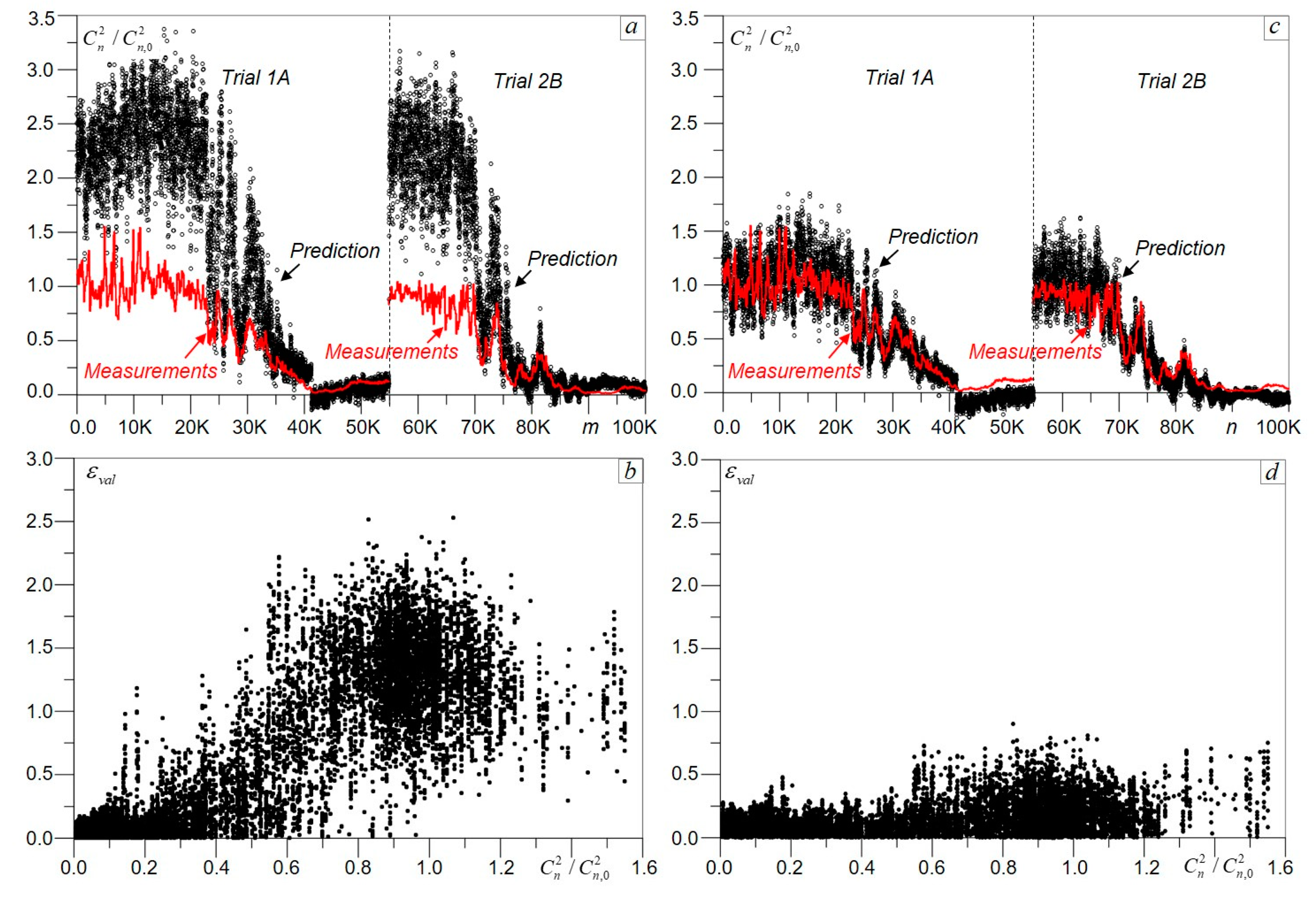
The results of DNN processing using the preliminary trained Cn^2Net models (N_model =20) are presented in Figure 7. The $C_n^2$ “measurement-vs.-prediction” plots in Figure 7a,c provide a comparison of measured and predicted $C_n^2$ values for the entire range of turbulence conditions observed during the experimental trials. The prediction error standard deviations ${\sigma }_{val}(c_n^2)={\epsilon }_{val}(c_n^2)/c_n^2$ for both ATM#1-V and ATM#2-V datasets are shown in Figure 7b,d as functions of the normalized refractive index structure parameter $c_n^2=C_n^2/C_{n,0}^2$.

For each $C_n^2$ measurement, the Cn^2Net processed $N_{\Delta T}$/2 images and computed equal number of the averaged over DNN models $C_n^2$ predictions that are shown in Figure 7 by dots (prediction dots). The density of the prediction dots is noticeably higher for the ATM#2 dataset (Figure 7c,d) that has twice as many scintillation images per each $C_n^2$ measurement and almost three times more $C_n^2$ data points compared with the ATM#1 dataset. The density of prediction dots in Figure 7b,d reflects the frequency of $C_n^2$ data point occurrence in the corresponding dataset.

Note that the prediction error standard deviation ${\sigma }_{val}$ is significantly higher for relatively weak turbulence ($C_n^2<0.2·C_{n,0}^2$). Under these conditions the characteristic size of turbulence-induced speckles approaches or even exceeds the optical receiver aperture size (see Figure 4, 1eft column) leading to a reduction in spatial features manifold of the scintillation images processed by DNN and resulting in ${\sigma }_{val}$ increase. A similar effect was observed with DNN processing of the SIM dataset (see Figure 6b).

The prediction error standard deviation inside the weak turbulence region can in principal be reduced by increasing the optical receiver aperture size. However, under weak turbulence and/or for relatively short propagation distances (even in strong turbulence), intensity scintillations diminish and hence cannot be utilized for accurate characterization of turbulence strength.

The intensity scintillation level is commonly characterized by the Rytov variance ${\sigma }_R^2=1.23C_n^2{k}^{7/6}{L}^{11/6}$, where $k=2\pi /\lambda$ [29]. For the experimental setting used for ATM dataset collection (see Section 2), ${\sigma }_R^2=10.9c_n^2$. The results in Figure 7b,d suggest that accurate (within 10–15%) $C_n^2$ prediction using Cn^2Net can only be achieved under conditions of relatively strong scintillations with Rytov variance ranging from ${\sigma }_R^2~1$ to ${\sigma }_R^2~20$. Note that this physics-imposed limitation can be overcome by utilizing for DNN-based data processing optical sensing characteristics that are more affected by atmospheric turbulence under weak scintillation conditions, such as short-exposure focal plane intensity patterns, turbulence-degraded images and wavefront sensing data.

However, under strong scintillations (${\sigma }_R^2>1$) an optical system (similar to as in Figure 1) composed of a remotely located laser beacon and optical receiver equipped with a camera capturing short-exposure intensity scintillation patterns, and DNN-based data processing hardware, can be utilized as a $C_n^2$ sensor for atmospheric turbulence characterization, similarly to conventional scintillometers. For convenience, such an optical system with DNN processing of scintillation images is referred to here as a Cn^2Net scintillometer.

Prior to measurements ($C_n^2$ prediction based on captured scintillation images), the Cn^2Net scintillometer should be side-by-side trained and validated with a calibrated (“trusted”) conventional $C_n^2$ sensor. This DNN training-validation phase also provides estimation of $C_n^2$ prediction error and defines the range of turbulence conditions for operation with an acceptable $C_n^2$ prediction accuracy.

Besides solely economic motivations (the Cn^2Net scintillometer may cost a fraction of the cost of current commercial instruments), this DNN-based $C_n^2$ sensor could also provide important new capabilities for atmospheric turbulence characterization.

To further explore both capabilities and limitations of atmospheric turbulence characterization with DNN processing of intensity scintillation images, we compared the defined by Equation (3) root mean square errors (RMSE) ${\epsilon }_{val}(c_n^2)$ for the datasets obtained in numerical simulations (SIM-KO-V) and atmospheric trials (ATM#1-V and ATM#2-V). The corresponding scatter plots are shown in Figure 8.

The prediction errors averaged across the entire $C_n^2$ range ${\overline{\epsilon }}_{val}$ and their standard deviations ${\sigma }_{\epsilon }$ computed using the data in Figure 8 are presented in

Table 2. Averaged prediction error ${\overline{\epsilon }}_{val}$ and its standard deviation ${\sigma }_{\epsilon }$ for the Cn^2Net trained using different datasets.

DNN Training Dataset	${\overline{\mathit{\epsilon }}}_{\mathit{v}\mathit{a}\mathit{l}}$	${\mathit{\sigma }}_{\mathit{\epsilon }}$	# ${\mathit{C}}_{\mathit{n}}^2$ Values	# Frames
SIM-KO-T	0.072	0.06	10,000	10,000
ATM#1-T	0.194	0.14	322	9668
ATM#2-T	0.09	0.08	940	56,443

.

Both ${\overline{\epsilon }}_{val}$ and ${\sigma }_{\epsilon }$ are the smallest for the SIM-KO dataset. The prediction error ${\overline{\epsilon }}_{val}$ for this dataset is correspondingly 2.7-fold and 1.25-fold smaller in comparison with the ATM#1 and ATM#2 datasets. The fact that $C_n^2$ prediction was more accurate for the ATM#2 dataset than the ATM#1 dataset is not surprising since the ATM#2 dataset contains significantly more instances (both $C_n^2$ values and scintillation images) used for Cn^2Net training than does the ATM#1 dataset.

A different question is why Cn^2Net training using a relatively small (10K) SIM-KO dataset resulted in a prediction RMSE that is 1.25-fold smaller in comparison with training on the ATM#2-T dataset that has a significantly larger number (56.4 K) of scintillation images?

To address this question first notice that a single scintillation image of the SIM-KO dataset corresponds to a single $C_n^2$ value, while in the ATM#1 and ATM#2 datasets a single measured $C_n^2$ value corresponds, respectively, to 30 and 60 scintillation images that were captured between sequential $C_n^2$ measurements.

This difference would not explain the observed increase in the prediction error in DNN processing of the experimental data if the statistical properties of all of these (corresponding to each single measured $C_n^2$ value) scintillation images are alike. On the contrary, we would expect a quite opposite effect: smaller prediction errors since more scintillation images were utilized for DNN training per a single $C_n^2$ value.

The observed prediction error increase with DNN processing of the ATM datasets could most likely be explained by the nonstationarity of atmospheric turbulence dynamics during the ΔT = 60 s. time interval between sequential $C_n^2$ measurements by the scintillometer.

During this time, the characteristic spatial features of turbulence-induced speckles in the scintillation images captured by the camera (e.g., characteristic size and contrast of speckles) could considerably evolve. Cn^2Net, which is trained based on analysis of these spatial features, would respond to these changes by predicting $C_n^2$ values that are different from those that were measured by the scintillometer. Since $C_n^2$ sensing with a conventional scintillometer is based on time-averaging of data acquired during the time interval between sequential measurements, this instrument principally cannot detect changes in turbulence that may occur during the averaging time.

On the other hand, the $C_n^2$ sensing rate of the scintillometer cannot be increased to match the camera frame rate without sacrificing the accuracy required for obtaining statistical characteristics based on time-averaging.

From this view point, the Cn^2Net scintillometer could provide significantly higher temporal resolution in $C_n^2$ sensing, which is highly desired for better understanding and prediction of atmospheric turbulence effects.

As an illustration consider Figure 9, which shows an eight-minute long (“time zoom”) extraction from the “measurement-vs.-prediction” plot in Figure 7, where the solid line and dots correspondingly show the measured by the scintillometer and predicted by the Cn^2Net $C_n^2$ values based on processing of the ATM#2 dataset. The dotted curve in this figure clearly displays changes in turbulence (in spatial features of turbulence-induced speckles) occurring between sequential $C_n^2$ measurements by the scintillometer. These changes in spatial features of speckles can be easily seen in the exemplary short exposure scintillation images in Figure 9 which were recorded during Δt = 20 s. between two subsequent $C_n^2$ measurements.

This example outlines the principal difficulties with Cn^2Net training by utilizing $C_n^2$ data recorded with a conventional (“trusted”) scintillometer as the “ground truth”. Such training could be “confusing” for the DNN when turbulence strength and, hence, spatial features of the scintillation images used in such training are rapidly changing between sequential $C_n^2$ measurements with conventional instruments having a relative low temporal resolution (from one to several minutes per single $C_n^2$ data point). An indication of such “misleading” DNN training is the significant increase in prediction errors under strong turbulence conditions ($C_n^2>C_{n,0}^2$), as seen in Figure 8b,c. Note that under these conditions the scintillometer recordings exhibit strong fluctuations (see Figure 7a,c) caused by non-stationarity of the turbulence dynamics at the time scale of the $C_n^2$ measurements.

The machine learning experiments with the ATM datasets described raise a question about the “right” dataset for DNN training, which could provide full advantage of the Cn^2Net scintillometer capabilities for real-time turbulence characterization. Such new capabilities in $C_n^2$ sensing are important for the development of a wide range of atmospheric optics systems including free-space optical communications, adaptive optics, directed energy, lidars etc.

6. Cn^2Net Scintillometer Training with SIM Datasets: Machine Learning-Based Turbulence Profiling

Assume that wave-optics numerical simulations could provide accurate modelling of laser beam propagation over any selected turbulence characterization site and, thus, can be utilized for the generation of sufficiently large SIM datasets for DNN training. A DNN that is trained at this SIM dataset (SIM-trained DNN) can then be further used for real-time processing of scintillation images and $C_n^2$ prediction at the selected site. In the case of Cn^2Net training using such SIM dataset, a “trusted” scintillometer for collection of the training data (ATM dataset) is not required. Furthermore, the SIM-trained Cn^2Net scintillometer could be further utilized at different propagation sites by simply computing a new SIM dataset specific for this site with corresponding Cn^2Net retraining.

There are, nevertheless, several potential issues with such Cn^2Net scintillometer training using SIM datasets. First, it is not always clear how accurately we can mimic laser beam propagation at any given turbulence characterization site in our numerical simulations. In other words, could we trust SIM datasets more than ATM datasets obtained using side-by-side $C_n^2$ measurements with a “trusted” scintillometer? Second, since there are several well-known atmospheric turbulence models, it is unclear which model to use for SIM datasets generation.

Third, there could be one more potential issue associated with frequently observed inhomogeneities of the refractive index structure parameter along the propagation path. This $C_n^2$ inhomogeneity is commonly accounted for in numerical simulations by applying one or another model to describe refractive index structure parameter dependence on the propagation distance $0\le z\le L$ ($C_n^2$-profile): $C_n^2(z)$ [30,31]. In the most known $C_n^2$-profile models (e.g., Hufnagel–Valley [32], SLC [33], Gurvich [34], etc.) the structure parameter is considered as a function dependent solely on propagation path elevation ($C_n^2$ vertical profile).

However, at propagation sites with complicated terrain features, the refractive index structure parameter could be inhomogeneous along all three geographical coordinates (elevation, longitude and altitude), which makes generation of SIM datasets a challenging problem. Some progress in the modeling of refraction index and $C_n^2$ fields dependent on 3D geographical coordinates and time has recently been made using numerical weather prediction (NWP) simulations [35,36,37]. The NWP approach could potentially be applied for generation of more accurate SIM datasets for DNN training.

In another approach considered here, the deep machine learning paradigm is applied to fine-tune a model-based $C_n^2$- profile to a selected turbulence characterization site by utilizing atmospheric sensing data acquired at this site (inference ATM dataset). In this case, DNN is initially trained on a SIM dataset corresponding to a specified $C_n^2$ profile model (e.g., uniform, or HV-21 $C_n^2$-altitude profile). The SIM-trained DNN is further applied for prediction (inference) of the experimentally measured $C_n^2$ values based on processing of scintillation images from the inference ATM dataset. The initial (model-based) $C_n^2$-profile is further modified to decrease prediction error obtained during the DNN inference phase.

This modification can be performed by adjusting a few tunable parameters that could be selected based on various factors including availability of additional information about terrain features and/or specific propagation site characteristics, weather conditions, etc. The modified $C_n^2$ profile can be further applied for generation of a new training dataset, DNN retraining and subsequent analysis of the $C_n^2$ prediction performance using the inference ATM dataset. This process of tunable parameter modification, DNN retraining and prediction performance evaluation could be repeated to achieve better matching of DNN prediction with actual (measured with a conventional scintillometer) $C_n^2$ data.

This general approach for $C_n^2$-profile tuning was analyzed in several cross-dataset machine learning experiments. For initial Cn^2Net training we used the SIM-KO-U dataset corresponding to the Kolmogorov turbulence model with $C_n^2$ values that were independent of propagation distance (uniform). Performance of the SIM-trained Cn^2Net was evaluated via processing of the scintillation images from the ATM#1 and ATM#2 datasets (inference datasets).

The results obtained for both inference datasets are presented in

Table 3. Averaged $C_n^2$ prediction error ${\overline{\epsilon }}_{val}$ and its standard deviation ${\sigma }_{\epsilon }$ for Cn^2Net models trained using simulated datasets corresponding to the Kolmogorov turbulence model with uniform (SIM-KO-U) and unevenly distributed (profiled) along the propagation path (SIM-KO-P) refractive index structure parameter. Predictions of the $C_n^2$ values measured with a scintillometer were performed in cross-dataset machine learning experiments using scintillation images from ATM#1 and ATM#2 inference datasets collected during the atmospheric sensing trials (see Section 2).

DNN Training/Inference (Validation) Dataset	${\overline{\mathit{\epsilon }}}_{\mathit{v}\mathit{a}\mathit{l}}$	${\mathit{\sigma }}_{\mathit{\epsilon }}$	# ${\mathit{C}}_{\mathit{n}}^2$ Values	# Frames
SIM-KO-U/ SIM-KO-U	0.072	0.06	10,000/ 10,000	10,000/ 10,000
SIM-KO-U/ SIM-KO-P	0.65	0.1	10,000/ 10,000	10,000/ 10,000
SIM-KO-U/ ATM#1	0.541	0.232	10,000/ 322	10,000/ 19,336
SIM-KO-P/ ATM#1	0.130	0.03	10,000/ 322	10,000/ 19,336
SIM-KO-U/ ATM#2	0.557	0.391	10,000 940	10,000 112,866
SIM-KO-P/ ATM#2	0.140	0.013	10,000 940	10,000 112,866

and illustrated in Figure 10 (for the ATM#2 dataset only). The measurement-vs.-prediction and prediction RMSE ${\epsilon }_{val}(c_n^2)$ plots in Figure 10a,b clearly indicate that training with the initial SIM-KO-U dataset provided poor performance in $C_n^2$ prediction. The prediction error $({\overline{\epsilon }}_{val}\approx 0.56)$ in this case was approximately 6.4-fold higher in comparison with the corresponding error obtained when the ATM#2 dataset was utilized for both DNN training and $C_n^2$ prediction (see Table 3). Similarly, high prediction error (${\overline{\epsilon }}_{val}\approx 0.54$) was observed when the SIM-KO-U-trained Cn^2Net was used to predict $C_n^2$ values using the ATM#1 inference dataset.

Such poor Cn^2Net performance during the inference phase can be explained by either inconsistency between the experimentally measured data and the SIM-KO-U data computed based on the Kolmogorov turbulence model, or by the possible impact of turbulence inhomogeneities along the propagation path in Figure 1, or by both.

First, we assumed that turbulence inhomogeneities rather than deviations from the Kolmogorov classical model were the reason for the Cn^2Net poor performance. This notion was motivated by the visible comparison between the computer simulated scintillation patterns and those captured during the atmospheric trials, as shown in Figure 4. In this figure the spatial structures of scintillation speckles from the SIM-KO-U and ATM#2 datasets are quite similar under the weak-to-medium turbulence conditions typical for measurements during early morning hours, but noticeably different under the strong turbulence conditions observed for data collection during a sunny afternoon (see right row in Figure 4). This mismatch between simulations and measurements under strong turbulence could be explained by turbulence enhancement in the vicinity of the laser beacon that was located on the flat rooftop surface of the VAMC building (see Figure 1).

The heated air flows generated on the roof surface are especially strong during sunny afternoon measurements (strong turbulence conditions), which may cause the turbulence enhancement for the propagation path region near the laser beacon and thus explain the observed mismatch in speckle structures.

To verify this hypothesis, we introduced a simple modification into the uniform $C_n^2$ profile that was originally used for SIM-KO-U dataset generation. In the wave-optics computer simulations of laser beacon beam propagation (see Section 3), we intentionally increased the strength of the two computer generated phase screens closest to the laser beacon by a factor of $\kappa \ge 1$ ($C_n^2$ profiling factor), while preserving the path-integrated $C_n^2$ values through an equivalent decrease in $C_n^2$ strength for the remaining eight phase screens. Note that the SIM-KO-U dataset corresponds to $\kappa ={\kappa }_0=1$ (uniform profile).

The initially uniform $C_n^2$ profile was modified through a set of Cn^2Net training-inference iterative steps. Each nth iteration of the $C_n^2$ profile modification included: (a) generation of a SIM-KO-P dataset corresponding to a profiling factor ${\kappa }_n={\kappa }_0+n\Delta \kappa$, where $\Delta \kappa =0.25$ is a selected profiling factor increment; (b) Cn^2Net training using a SIM-KO-P dataset computed at the nth iteration; (c) evaluation of the trained DNN at ATM inference datasets; and (d) comparison of averaged prediction errors ${\overline{\epsilon }}_{val}({\kappa }_n)$ with the corresponding errors obtained during the previous training-inference step. The steps (a)–(d) were repeated until the smallest prediction error ${\overline{\epsilon }}_{val}({\kappa }_n)$ was obtained.

The $C_n^2$ profile tuning results are illustrated in Figure 10c,d. Both the measurement-vs.-prediction and prediction RMSE ${\epsilon }_{val}(c_n^2)$ plots indicate a significant improvement in $C_n^2$ prediction accuracy, which was achieved with the Cn^2Net training using the SIM-KO-P dataset obtained with the optimal profiling factor κ = 2.5.

The averaged prediction errors ${\overline{\epsilon }}_{val}$ and their standard deviations ${\sigma }_{\epsilon }$ obtained in the described cross-dataset machine learning experiments are summarized in Table 3. For both inference datasets examined, the smallest prediction errors (${\overline{\epsilon }}_{val}$ = 0.13 for ATM#1 and ${\overline{\epsilon }}_{val}$ = 0.14 for ATM#2) were achieved with the profiling factor κ = 2.5. These errors (see Table 3) are comparable with the corresponding errors obtained when both training and validation of the Cn^2Net were performed using subsets of the same dataset: either SIM-KO-U or ATM#1 or ATM#2 datasets. Note that tunable parameters of the $C_n^2$ profile could potentially be included into a set of DNN trainable parameters and be defined during the DNN training-validation phase.

To understand how the machine learning-based $C_n^2$ profiling described here affects the characteristic spatial features of scintillations, compare the scintillation images shown in Figure 11 resulting from different DNN training (SIM-KO-U vs. SIM-KO-P) and inference (ATM#2) datasets. Under weak-to-medium turbulence conditions the spatial structures of scintillation speckles (two left column images in Figure 11) are similar for all three datasets. At the same time, under strong turbulence (images in the right two columns) one can easily observe a noticeable difference in the characteristic size of speckles between images captured during the experimental trial (ATM#2 dataset) and computed using a uniform (SIM-KO-U) $C_n^2$ profile (κ = 1.0). This difference practically vanishes in scintillation images taken from the SIM-KO-P (κ = 2.5) dataset which were obtained during machine learning-based $C_n^2$ profiling. The spatial structures of speckles in images belonging to the ATM#2 and SIM-KO-P datasets (two bottom rows in Figure 11) are alike under all turbulence conditions observed in experiments and mimicked in wave-optics numerical simulations.

The turbulence profiling example described here illustrates the potentials for application of the deep machine learning concept to atmospheric turbulence sensing and characterization.

7. Turbulence Models Evaluation via Machine Learning

In the training-inference machine learning experiments discussed in Section 6 we only used the Kolmogorov power spectrum model for SIM dataset generation. Could we improve performance of the SIM-trained Cn^2Net by utilizing a different atmospheric turbulence model for SIM dataset generation? A broader question to ask is if the machine learning framework could be applied for theoretical models assessment, evaluation of their accuracy and applicability to diverse atmospheric propagation environments?

Since we already evaluated performance of the SIM-KO-trained Cn^2Net in prediction of $C_n^2$ values using ATM#1 and ATM#2 inference datasets, and since, as discussed in Section 5, $C_n^2$ measurements do not always reflect in-situ changes in atmospheric turbulence dynamics, it would be rational to compare different power spectrum models in cross-dataset training-inference machine learning experiments using the SIM-KO-trained Cn^2Net as a reference.

In the analysis presented in this section, both training and inference datasets were generated using the split-step operator technique described in Section 3. Turbulence-induced refractive index random fluctuations were represented by sets of statistically homogeneous, isotropic thin phase screens obeying one of the following well-known power spectrum models (see Appendix A): Kolmogorov [1], Tatarskii, Von Karman and Andrews [2,29]. The corresponding SIM datasets are referred to as SIM-KO, SIM-TA, SIM-VK and SIM-AN. The refractive index structure parameter $C_n^2$ was assumed to be constant along the propagation path (uniform $C_n^2$ profile). The Kolmogorov SIM-KO dataset was used for Cn^2Net training, and the other datasets for inference. Note that the inner $l_0$ and outer $L_0$ scale parameters for the Von Karman and Tatarskii power spectrum models (see Appendix A) were equal to the numerical grid pixel size ($l_0$= 1 mm) and overall grid dimension ($L_0$ = 1.0 m), respectively.

We also considered two additional inference datasets generated for the so-called non-Kolmogorov power spectrum model (SIM-NK datasets).

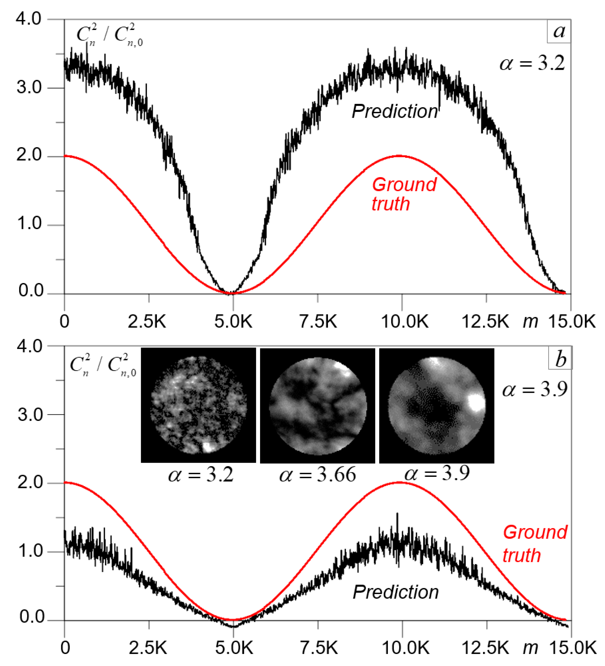
The results of the Cn^2Net cross-dataset training-inference experiments with different inference SIM datasets are presented in

Table 4. Averaged prediction errors ${\overline{\epsilon }}_{val}$ and their standard deviations ${\sigma }_{\epsilon }$ computed in the cross-dataset Cn^2Net training-inference experiments with SIM-KO dataset used for training, and SIM-Tatarskii (TA), SIM-Von Karman (VK), SIM-Andrews (AN) and SIM-NK datasets for inference ($C_n^2$ prediction).

Inference Dataset	SIM-TA	SIM-VK	SIM-AN	SIM-NK α = 3.2/α = 3.9
${\overline{\epsilon }}_{val}$	0.077	0.091	0.093	1.16/0.45
${\sigma }_{\epsilon }$	0.079	0.083	0.091	0.54/0.31

and illustrated in Figure 12. In all cases the datasets were composed of 15,000 computer simulated scintillation images corresponding to the cosine-type $C_n^2(m)$ dependence described by Equation (1) and shown in Figure 12 as the ground truth curve. DNN performance was evaluated using prediction errors ${\overline{\epsilon }}_{val}$ averaged across the entire $C_n^2$ range and their standard deviations ${\sigma }_{\epsilon }$.

To evaluate the DNN ability to distinguish between scintillation images generated using different power spectrum models, compare the prediction errors presented in Table 4 obtained in the cross-dataset training-inference experiments with the corresponding value ${\overline{\epsilon }}_{val}$ = 0.072 computed in training-validation simulations when non-overlapping subsets of the SIM-KO dataset were used for both Cn^2Net training and $C_n^2$ prediction (validation). The observed relatively small (<3%) difference in the prediction errors and their standard deviations suggests that scintillation images corresponding to the Kolmogorov, Tatarskii, Von Karman and Andrews turbulence models have nearly identical (undistinguished by the Cn^2Net) spatial features, and from this viewpoint are alike.

At the same time, DNN processing of scintillation images corresponding to the non-Kolmogorov turbulence power spectrum model (images from SIM-NK inference datasets) resulted in enormously large (>600%) errors. This mismatch between the ground truth and predicted $C_n^2$ values based on processing of the SIM-NK inference datasets is clearly seen in Figure 12.

The representative scintillation images in Figure 12 additionally demonstrate the clearly visible distinction in speckle pattern structures in the scintillation images corresponding to the Kolmogorov $(\alpha =11/3\approx 3.66)$ and non-Kolmogorov ($\alpha =3.2$ and $\alpha =3.9$) power spectrum models.

In addition to comparison and evaluation of different atmospheric turbulence models, the machine learning concept can also be applied to analyze the impact of the parameters upon which these models may depend.

Consider as an example DNN-based analysis of the turbulence inner scale impact on the spatial features of speckles in the scintillation images. The turbulence inner $l_0$ and outer $L_0$ scales are key parameters for the Von Karman and Andrews turbulence models (see Appendix A). For this analysis we generated a set of SIM-VK datasets corresponding to the Von Karman turbulence model with varied inner scale values ranging from $l_0 =1.0$ mm to $l_0 =16.0$ mm, and a fixed outer scale parameter $L_0$ = 1.0 m. Cn^2Net was trained using the SIM-KO dataset while the generated SIM-VK datasets with different $l_0$ were used for the $C_n^2$ true value predictions (inference).

Results of the corresponding machine learning experiments are summarized in

Table 5. Evaluation of turbulence inner $l_0$ and outer $L_0$ scales impact on averaged $C_n^2$ prediction error ${\overline{\epsilon }}_{val}$ in the cross-dataset training-inference machine learning experiments with Cn^2Net training performed using the SIM-KO dataset (Kolmogorov turbulence model) and inference ($C_n^2$ prediction) using the SIM-VK datasets (Von Karman power spectrum model). The first row corresponds to the deep neural network (DNN) training and prediction using SIM-KO datasets.

${\mathit{l}}_0\left(\mathbf{mm}\right)$	${\mathit{L}}_0\left(\mathbf{m}\right)$	${\overline{\mathit{\epsilon }}}_{\mathit{v}\mathit{a}\mathit{l}}$
0	Infinity	0.072
1.0	1.0	0.091
4.0	1.0	0.094
8.0	1.0	0.170
16.0	1.0	0.380
1.0	0.25	0.10
1.0	0.5	0.09
1.0	2.0	0.08
1.0	4.0	0.074

by averaged prediction errors ${\overline{\epsilon }}_{val}.$ As expected, the smallest difference between ground-truth and predicted $C_n^2$ values was achieved with the SIM-VK inference dataset computed for the smallest turbulence inner scale $l_0 =1.0$ mm corresponding to the numerical grid pixel size. This result is not a surprise since the DNN was trained with the SIM-KO dataset, while both the Von Karman and Kolmogorov spectra coincide for $l_0=0$ and $L_0 =\infty$ (first row in Table 5). When $l_0$ was increased, the accuracy in $C_n^2$ prediction declined and the corresponding averaged prediction error ${\overline{\epsilon }}_{val}$ increased. The rate in prediction error increase characterizes the sensitivity of spatial features in scintillations to the turbulence inner scale. Variations in $l_0$ within a few millimeters (from $l_0 =1.0$ mm to $l_0 =4.0$ mm) only marginally effected DNN performance and, hence, spatial features of the scintillation patterns utilized by Cn^2Net for $C_n^2$ prediction. With further turbulence inner scale $l_0$ increase ($l_0 =8.0$ mm and $l_0 =16.0$ mm), discrepancy between the true and predicted $C_n^2$ values was quite obvious.

Similar machine learning experiments were performed to estimate the impact of the turbulence outer scale $L_0$ in the Von Karman power spectrum model on scintillation patterns. In this study the turbulence outer scale $L_0$ was varied from $L_0$$=0.25$ m to $L_0=4$ m. The obtained results (see Table 5) demonstrated minor change in the $C_n^2$ prediction error that increased to about 5% with decrease in outer scale up to 0.25 m. These results indicate that outer scale variation within a reasonable (from physics viewpoint) range does not significantly affect spatial features of speckles in the scintillation images.

8. Concluding Remarks and Forthcoming Research Directions

In this paper, a deep machine learning computational framework is applied for prediction of the atmospheric turbulence refractive index structure parameter $C_n^2$ based on DNN processing of short exposure images of turbulence-induced laser beam intensity scintillations. To support the DNN model development and machine learning experiments, several datasets composed of large numbers of instances (scintillation images and the corresponding $C_n^2$ values) were collected during several atmospheric measurement trials over a 7 km propagation path, and computer-generated using wave-optics numerical simulations to imitate the experimental trials.

A deep convolutional neural network model (Cn^2Net) containing about 45,000 trainable parameters was developed and optimized via minimization of the $C_n^2$ prediction error for the entire range of turbulence strength variations observed during the measurement trials. Prediction of a single $C_n^2$ data point by a fully trained Cn^2Net model required about 0.14 sec, which provides capabilities for high temporal resolution (about seven or more data points per second) $C_n^2$ measurements.

The developed Cn^2Net model was applied for:

• prediction of the data obtained in the atmospheric measurement trials by processing of experimentally captured scintillation images never used for the Cn^2Net training;
• prediction of values recorded in the experimental trials by the Cn^2Net model trained on computer-generated scintillation images;
• turbulence profiling by iterative adjustments of a model-based profile by utilizing the measured data;
• comparison of the most prominent atmospheric turbulence models, and the analysis of their parameters impact (inner and outer scales) on scintillations.

In this study we show that an optical system comprised of a remotely located laser beacon and an optical receiver acquiring short-exposure intensity scintillation patterns digitally processed with a specially designed and trained DNN, can be utilized as a sensor (Cn^2Net scintillometer) for in-situ atmospheric turbulence characterization. Such a DNN-based $C_n^2$ sensor could be especially efficient for turbulence characterization over relatively long atmospheric propagation paths that are characterized by strong scintillations (Rytov variance ${\sigma }_R^2>1$). Note that conventional instruments for $C_n^2$ monitoring do not provide accurate measurements in strong (saturated) scintillation regimes.

The Cn^2Net scintillometer is less effective when scintillations are relatively weak (low $C_n^2$ and/or short propagation path length). In this case, intensity distributions at an optical receiver pupil are relatively weakly effected by the turbulence-induced wavefront aberrations due to an insufficiently long propagation (diffraction) distance and/or too weak turbulence. For the same reason, the Cn^2Net scintillometer has low sensitivity to turbulence layers located near the optical receiver and, hence, cannot provide accurate turbulence profiling along the entire propagation path.

However, the machine learning based atmospheric sensing concept proposed here can be equally applied to optical systems whose performance is strongly affected by turbulence layers located near the optical receiver (e.g., wavefront sensors, directed energy, power beaming, imaging and free-space laser communication systems). At the same time, the measured output optical characteristics in these systems can be insufficiently sensitive to remotely located turbulence layers and for this reason cannot be efficient for turbulence characterization in strong scintillation conditions.

One of the major attractions of the machine learning approach for atmospheric turbulence characterization is that it offers a wide range of capabilities for real-time fusion of data flows coming from various optical and meteorological sensors [38,39]. To better reveal the complexity of atmospheric turbulence dynamics, the sensor outputs should be differently affected by atmospheric turbulence; e.g., have enhanced sensitivity to the location of turbulence layers, or to specific spatial and/or temporal characteristics of atmospheric refractive index inhomogeneities, or changes in atmospheric refractivity, visibility, etc. From this viewpoint diversity in sensing data that enter a DNN-based signal processing system is highly desired.

Although in this paper we focused solely on sensing of the refractive index structure parameter $C_n^2,$ machine learning-inspired atmospheric sensors could also selectively target different atmospheric turbulence characteristics (e.g., Fried, or Rytov parameters, Strehl ratio, image sharpness, received signal fading duration, etc. [29,40]) that more directly characterize the performance of one or another electro-optical system. This eliminates the need for computing these characteristics (performance metrics) using theoretical expressions that link performance metrics with the characteristics of the propagation path, optical system parameters and characterized by $C_n^2$ turbulence conditions. Note that in many cases such expressions derived from the theory either do not exist or can only be obtained under assumptions that are not always fulfilled.

These arguments emphasize another major advantage of the machine learning-enhanced atmospheric sensing approach: it provides assumption-free prediction (with a properly trained DNN) of specific performance metrics and/or those most important for various types of optical systems.

Since machine-learning-inspired atmospheric sensing is based on extraction of spatial or temporal (or both) features from the incoming sensing data, rather than on time-averaging of data acquired during the time interval between sequential measurements as in conventional instruments used for turbulence characterization, DNN-enhanced sensors can potentially provide much higher temporal resolution and be capable of real-time detection of the changes occurring in atmosphere under different turbulence conditions.

This capability is especially important for prediction and in-situ adjustment of electro-optical systems parameters based on atmospheric sensing information. For example, prediction of coming deep signal fading in a free-space laser communication system could be used to minimize losses in the throughput data. In adaptive optics systems, in-situ prediction of turbulence conditions that may occur within the time scale of a few seconds may provide opportunities to correspondingly adjust wavefront sensing and control system parameters for optimal system performance.

Machine learning-enhanced atmospheric sensing may also transform wave-optics numerical modeling and simulation tools from its current supporting role of electro-optical systems performance assessment under various environments into a key role of being an integrated part of the sensing system responsible for the DNN topology, parameter optimization and training.

Another important role machine learning could play for a wide range of atmospheric sensing applications is related to calibration of different sensors. “Agreement” between different sensor types, for example for $C_n^2$ measurements, is currently difficult to achieve even if these sensors operate side-by-side to simultaneously take measurements at the same atmospheric propagation site. This is not a surprise, as the operational principles of different sensors are commonly based on different assumptions and formulas that are derived from atmospheric turbulence theory and link $C_n^2$ with the statistical characteristics of measured signals. With the machine learning-enhanced atmospheric sensing approach that is based on extraction of spatial and temporal features of inputting DNN sensory information, rather than obtaining the “right” statistically averaged characteristics, it would be more straightforward to calibrate different sensors against a “reference” machine learning-based sensing system utilizing a “standard” topology DNN with identical parameters and training datasets.