Abstract
The current distribution of the grounding electrode in a high-voltage direct current (HVDC) transmission system affects the state of power equipment in its vicinity, which depends on the soil resistivity and shape of the grounding electrode. In this paper, current distribution in the vicinity of an ±800 kV grounding electrode is investigated by simulation and experiments. Firstly, the model to calculate the current distribution with two typical frozen soils is set up, and simulation models and experimental platforms are established; meanwhile, the finite element method (FEM) is used to calculate the current and potential dispersion of linear, cross-shaped, and ring-shaped grounding electrodes in the simulation models. After obtaining the lab current data from the simulation, an innovative method based on a “drainage wire” with a Hall sensor is proposed to measure the current in an experimental setup. The results show that current and potential distribution characteristics are related to the shape of the grounding electrode and soil resistivity. Meanwhile, the current measurement scheme can measure the current in soil with a lower error. This article concludes that these two typical models can reduce the complexity of frozen soil analysis, and the measurement scheme can accurately monitor the current to reduce the damage to the surrounding power equipment.
1. Introduction
HVDC transmission systems have reached a voltage level of ±1100 kV, and the stable operation of the grounding electrode is critical for the reliable operation of HVDC systems [1]. The grounding electrode can not only form a loop when the DC system is operating in a single-pole operating status but also balances the neutral point potential of the converter transformer [2,3]. Besides, soil resistivity determines the current distribution, hence it is necessary to investigate the current distribution in the vicinity of the grounding electrode considering different soil textures [4].
The disadvantages of the HVDC transmission project are that the electrical parameters of the grounding electrode still rely on the manual collection and the degree of automation is insufficient [5]. The resistivity in the soil where the grounding electrode is located will change with the changes in environmental temperature and humidity, while there are frozen soil and seasonally frozen soil in many areas [6]. At present, many scholars have conducted in-depth research on these topics. Zhang et al. used the complex image method to calculate the potential distribution of multi-layer soil between grounding electrodes in a DC transmission system and analyzed the influence of deep layers such as the crust, mantle, and core for the potential distribution on Earth’s surface [7]. Liu et al. used the finite element method to study the surface potential distribution of typical soil models and multi-layer soil models [8]. Yang et al. developed a grounding electrode monitoring system that can collect the grounding current, temperature, and humidity at the grounding electrode site [9].
The finite element method has been frequently used to calculate the current distribution in the soil near the grounding electrode [10,11,12,13,14]. The finite element method has been widely used in the study of grounding electrode current characteristics, but to better analyze it in engineering, real-time current monitoring is also needed. If a large DC flows from the grounding electrode into the soil, it will harm the surrounding metal pipes, transformers and other power equipment, and even humans or livestock. Therefore, it is necessary to study and design a weak current measurement device to be placed in the soil around the grounding electrode.
In this paper, three-layer and mixed-layer soil models are proposed to calculate the current distribution in the vicinity of the grounding electrode, which considers the influence of frozen soil and the electric field. Experiments were set up to simulate the current distribution for extremely cold weather conditions, in which different magnitudes of the current flow into the ground, and the depth of the grounding electrode, the resistivity of the soil, and the location of the current measuring device were investigated. Finally, a “drainage wire” with a Hall sensor-based method is proposed to measure the leakage current in the soil under the simulation test platform, and a weak current measurement device range from 0 to 50 mA is designed. Then, the reliability and accuracy of the measuring device are verified.
2. Current Distribution Calculation Model for Frozen Soil
Figure 1 is the schematic diagram for three-layer frozen soil, where set I is the current flowing into the ground. The entire ground can be simply divided into two parts, one of which includes the point current source, and the second is the area that does not contain the point current source [15,16,17]. The current distribution in region 1 satisfies the Poisson equation, and it satisfies the Laplace equation in regions 2–6.
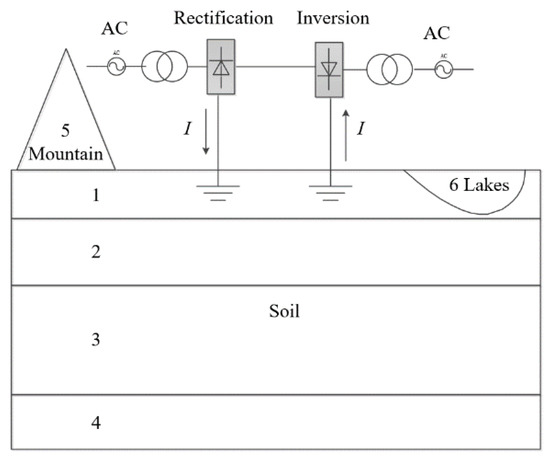
Figure 1.
Mixed-layer soil model. The resistivity of each layer of soil in regions 1–4 is different, and the grounding electrode is buried in area 1. Region 5 is a mountain that may exist in the surrounding environment, and region 6 is a lake, river, etc.
Besides, each region has different soil parameters in Figure 1, and the conductivity is in the order of σ1–σ6. In regions 2–6, where there is no point current source, the electric field equation is as follows. Here, V is the electric potential.
Since there is a current source in region 1, the equation in this field must be considered separately. First, define the unit point charge density function as follows. ρ is the unit point charge density.
This function is the charge density of a unit point at point x′. Further, δ(x) is defined as follows:
In the area where a point current source exists, the following relationship can be obtained. Here, I is the current, J is the current density, s is the surface through which the current flows, and Ω is the calculation area.
For
The following formula can be derived:
Then, the electric field equation in region 1 can be written as follows. Here, is the soil resistivity.
At the outer boundary: V = 0. The surface above region 1 and region 1 has a relationship: dv/dn = 0, where n is the direction of the outer normal, pointing from region 1 to the outside. Assuming that the soil labels in different layers of the model are i and j, the boundary conditions are
Using the abovementioned electric field equations and boundary conditions based on the finite element Galerkin method, the differential equation of the soil electric field can be obtained using the weighted residuals method.
3. Calculation and Analysis of Current Distribution
3.1. Frozen Soil Model Setup
Linear, cross-shaped, and ring-shaped grounding electrodes are frequently used in HVDC transmission systems [18]. The simulation results show that these two typical soil models can accurately reflect the characteristics of grounding electrode dispersion in a frozen soil environment [19,20]. In order to conduct a laboratory test, lab parameters for two typical frozen soil models are shown in Table 1, while two typical frozen soil models and dimensions of the grounding electrodes are shown in Figure 2.

Table 1.
Lab parameters for two typical frozen soil models.
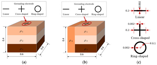
Figure 2.
Two typical frozen soil models and three typical grounding electrode sizes. (a) Three-layer soil model with three different grounding electrodes, the thickness of each layer is the same; (b) mixed-layer soil model with three different grounding electrodes, the soil width of the vertical layered soil is 0.2m; (c) the dimensions of linear, cross-shaped, and ring-shaped grounding electrodes are marked in detail.
In the model, are the conductivities for each layer of soil in the horizontal and vertical layers. The three-layer soil model reflects the distribution of soil conductivity in different layers under normal soil conditions, and the conductivity decreases from top to bottom. Meanwhile, in the mixed-layer soil, soil conductivity of the middle layer is highest and is the soil conductivity of the geological environment with faults, such as lakes, cliffs, and other different soil environments.
To facilitate data collection and statistical analysis of current and voltage, the X and Y coordinate directions were redefined during the data analysis using the soil model, as shown in Figure 3.
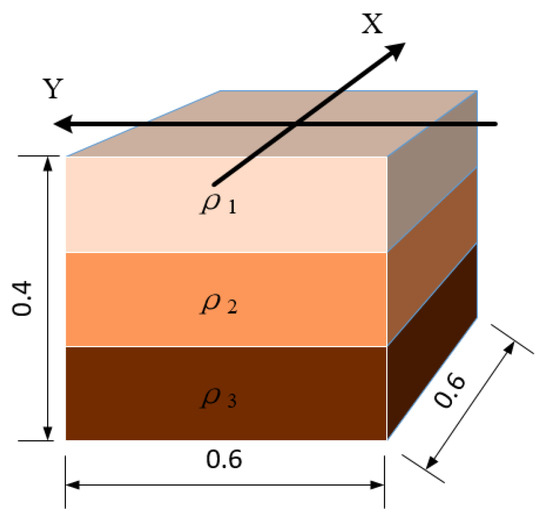
Figure 3.
Frozen soil model with X and Y coordinate directions.
3.2. Calculation of Electric Field
According to the distribution of soil electrical conductivity in the frozen soil environment in Inner Mongolia, two typical frozen soil models were established. In this article, the measurement cross-section of current density and potential distribution is located at 0.05 m below the ground surface and the parameters used in the simulation are shown in Table 2 and Table 3.
Table 2.
Parameters for the three-layer soil model.
Table 3.
Parameters for the mixed-layer soil model.
The current density and potential distribution in the three-layer soil with linear, cross-shaped, and ring-shaped grounding electrodes are shown in Figure 4.
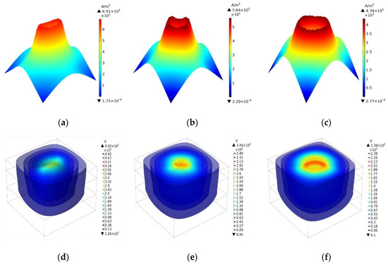
Figure 4.
Current density and potential distribution with different grounding electrodes. (a) Current density for linear grounding electrode; (b) current density for cross-shaped grounding electrode; (c) current density for ring-shaped grounding electrode; (d) potential distribution for linear grounding electrode; (e) potential distribution for cross-shaped grounding electrode; (f) potential distribution for ring-shaped grounding electrode.
The current density and potential distribution of the linear grounding electrode are the highest, reaching 69.1 A/m2 and 492 V, respectively. Meanwhile, the current and potential of the ring-shaped grounding electrode are the lowest, reaching 43.4 A/m2 and 238 V, respectively.
Furthermore, the current density and potential distribution under the mixed-layer soil model for linear, cross-shaped, and ring-shaped grounding electrodes are shown in Figure 5.
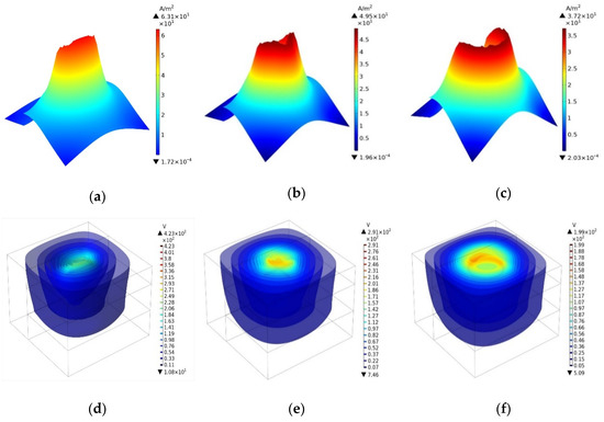
Figure 5.
Current density and potential distribution with different grounding electrodes. (a) Current density for linear grounding electrode; (b) current density for cross-shaped grounding electrode; (c) current density for ring-shaped grounding electrode; (d) potential distribution for linear grounding electrode; (e) potential distribution for cross-shaped grounding electrode; (f) potential distribution for ring-shaped grounding electrode.
Similarly, under the mixed-layer soil model, the current density and potential distribution of the linear grounding electrode are still the highest, which are 63.1 A/m2 and 423 V, respectively. Meanwhile, the values of the cross-shaped grounding electrode are 49.5 A/m2 and 291 V and the values of the ring-shaped grounding electrode are 37.2 A/m2 and 199 V, respectively.
We conclude that the ring-shaped grounding electrode has the best dispersion characteristics, the cross-shaped grounding electrode has the second best dispersion characteristics, and the linear grounding electrode has the worst dispersion characteristics.
3.3. Current Density and Potential Distribution
3.3.1. Three-layer Soil Model
In order to analyze the distribution characteristics of current density and potential value on the redefined X and Y coordinate planes, 130 sets of data are taken between 0 and 0.6m in the X and Y coordinate directions. Figure 6, Figure 7 and Figure 8 are the curves of the current density and potential of the linear, cross-shaped, and ring-shaped grounding electrodes under the three-layer soil model. The distribution curves in Figure 7 and Figure 8 almost completely coincide, so a dot-line plot is adopted for graphing purposes.
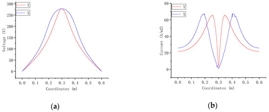
Figure 6.
Current density and potential distribution curves for the linear grounding electrode. (a) Potential distribution curves in the X and Y directions; (b) current density distribution curves in the X and Y directions.
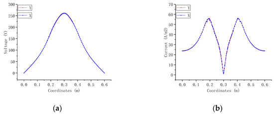
Figure 7.
Current density and potential distribution curves for the cross-shaped grounding electrode. (a) Potential distribution curves in the X and Y directions; (b) current density distribution curves in the X and Y directions.
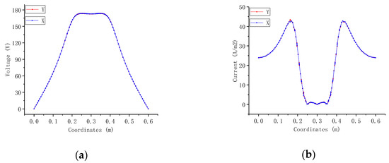
Figure 8.
Current density and potential distribution curves for the ring-shaped grounding electrode. (a) Potential distribution curves in the X and Y directions; (b) current density distribution curves in the X and Y directions.
The following analysis can be obtained from the current density and potential distribution curves of different grounding electrodes under the three-layer soil model:
For the linear grounding electrode, the maximum current density is about 67.4 A/m2, and the highest value is probably located at the surface directly above the two ends of the linear grounding electrode. The current peak value of 65.9 A/m2 also appears at the position where the Y coordinate is located at 0.25 and 0.35 m. At the boundary of the model, the current density drops to 25 A/m2. Secondly, the maximum potential is on the ground surface directly above the center of the linear grounding electrode, and the peak value is about 278 V.
The maximum current density of the cross-shaped grounding electrode is about 55.9 A/m2, and the highest value is located where the X coordinate is 0.2 and 0.4 m, while the Y coordinate is 0.2 and 0.4 m. Besides, the maximum potential is located on the ground surface directly above the center of the cross-shaped grounding electrode body, and the peak value is about 261 V.
For the ring-shaped grounding electrode, the maximum current density is about 43 A/m2, which is a circular area about 0.15 m from the center point. In a circular region of 0.05 m from the center, the surface current density is close to 0, and there are two smaller current peaks of about 1 A/m2. At the boundary of the soil model, the current density drops to 24 A/m2. On the other hand, the maximum potential is about 173 V on the ground surface directly above the ring-shaped grounding electrode body.
For the cross-shaped and ring-shaped grounding electrodes, the current density and potential distribution curves in both X and Y coordinates are completely overlapped. The reason for this overlapping is that the cross-shaped and ring-shaped grounding electrodes are completely symmetrical. Further, the surface current density directly above the center of the three grounding electrodes’ bodies is close to 0. Meanwhile, at the boundary of the soil model, the surface potential drops to 0.
3.3.2. Mixed-Layer Soil Model
Figure 9, Figure 10 and Figure 11 are the current density and potential curves of the linear, cross-shaped, and ring-shaped grounding electrodes under the mixed-layer soil model.
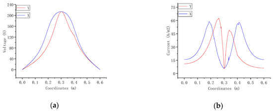
Figure 9.
Current density and potential distribution curves for the linear grounding electrode. (a) Potential distribution curves in the X and Y directions; (b) current density distribution curves in the X and Y directions.
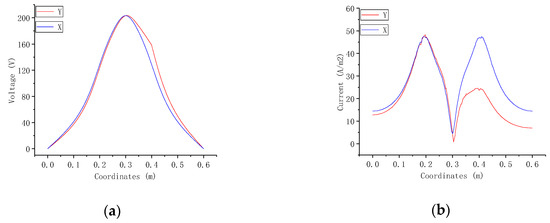
Figure 10.
Current density and potential distribution curves for the cross-shaped grounding electrode. (a) Potential distribution curves in the X and Y directions; (b) current density distribution curves in the X and Y directions.
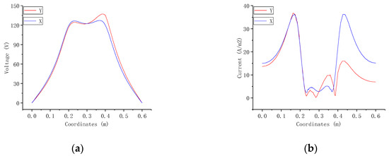
Figure 11.
Current density and potential distribution curves for the ring-shaped grounding electrode. (a) Potential distribution curves in the X and Y directions; (b) current density distribution curves in the X and Y directions.
Comparing with the three-layer soil model, the analysis results of the three grounding electrodes under the mixed-layer soil model are as follows:
For all three grounding electrodes, there is a sudden change in the current density and potential curves in the Y-axis direction. For the linear grounding electrode, the current peak drops to 49.1 A/m2 at the position where the Y coordinate is located at 0.35 m. For the cross-shaped grounding electrode, the current peak drops to 24.6 A/m2 at the position where the Y coordinate is located at 0.4 m. As for the ring-shaped grounding electrode, the peak value on the fault plane is 16 A/m2 and there are also two peaks of the current, with values of about 4 and 10 A/m2. Moreover, the potential of these three grounding electrodes has a small increase in the fault plane, all located at the Y coordinate of 0.4 m.
From the point of view, the values of current and voltage under the linear grounding electrodes are the highest, that is, the dispersion characteristic is the worst. The dispersion characteristic of the cross-shaped grounding electrode is the second highest, while the current and voltage of the ring-shaped grounding electrode are the lowest, indicating that the dispersion characteristic of the ring-shaped grounding electrode is best under the same geological conditions. Comparing with the linear grounding electrode, the ring-shaped grounding electrode can reduce the current and voltage in the soil near the grounding electrode by about 35–40%. In order to achieve a better dispersion effect and to reduce the damage to the surrounding power equipment, it is highly suggested to select the ring-shaped grounding electrode.
The above simulation research was conducted to perform equivalent reduction processing on the actual grounding electrode environment, which reduces the depth of the grounding electrode, the size of the earth, and the magnitude of the current. In order to verify the reliability of the above simulation, we carried out a corresponding laboratory simulation experiment in the next chapter.
4. Grounding Electrode Current Distribution Measurement
4.1. A “Drainage Wire”-Based Measurement Scheme
It is impossible to directly measure the DC when it overflows into the soil. Therefore, it is necessary to use a carrier to lead the soil current to the medium, then measure the current in the medium, so that the current can be indirectly measured and monitored [21]. Therefore, this paper proposes a measurement scheme based on a “drainage wire” with a Hall sensor to capture and measure the weak current in the soil near the grounding electrode. We select a copper drain rod as the current carrier in soil, which can drain the current in soil by laying the “drainage wire” in the soil [22,23,24].
According to Biot–Saavart’s law and Figure 12b, the current in the soil near the grounding electrode can be collected on the “drainage wire”.
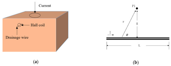
Figure 12.
A schematic of measuring the current in the soil. (a) The scheme of how the Hall sensor and “drainage wire” are placed in the soil; (b) a magnetic field generated by a finite-length conductor at a point.
It can be deduced that the expression of the magnetic field B generated by a conductor of length L at a point P1 at a vertical distance R from its center is
where P1 is the measurement point, L is the length of the conductor, I is the current flowing through the conductor, and R is the vertical distance.
4.2. Measurement Setup
Furthermore, we manufactured a device to measure leakage current in the soil near the grounding electrode, and a 0–50 mA range of the Hall DC sensor was selected for current measurement.
In Figure 13, a soil model is established by selecting a specific area in a certain environment around the grounding electrode. Firstly, we set up a simulation test platform in the laboratory, selected multiple measurement points, and buried sensors and the “drainage wire” at a certain depth in the soil. Secondly, the current collected by the sensor was transmitted to a single-chip microcomputer, which is the core of the weak current measuring device. Then, we added a heating module to make sure it could work normally under extremely cold conditions. Finally, the sensor data were transmitted to the server through the GSM (Global System for Mobile Communications) for establishing a complete grounding electrode database. The staff checked the detection data on the server or monitored the changes in all sensor parameters by mobile devices with remote distance.
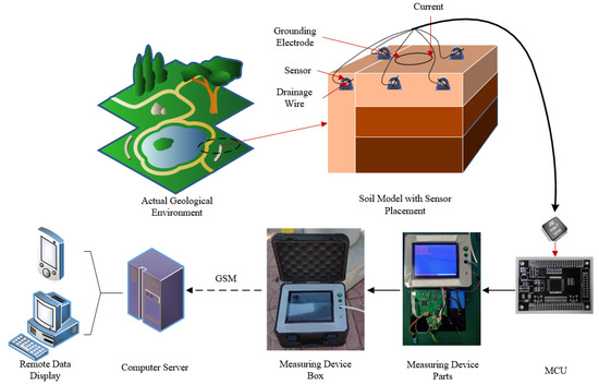
Figure 13.
Schematic of the leakage current measuring scheme.
Here, a DC power supply with 10 A current and 1000 W power was connected to the grounding electrode through a power resistance. Then, the current was spread into the soil and flowed back to the negative pole of the power supply through the container wall.
Moreover, we added water to each layer of soil according to Table 4 to realize soil structures with different resistivities [25,26]. Hence, a three-layer soil model and a mixed-layer soil model were built. The scene of the experimental measurement is shown in Figure 14b,c, and the monitoring interface of current and soil environmental temperature and humidity is shown in Figure 14d. The historical data of the current measurement were stored in a memory card, and a historical data curve can be used to observe the change in the leakage current at different locations in the soil.
Table 4.
Parameters for the mixed-layer soil model.
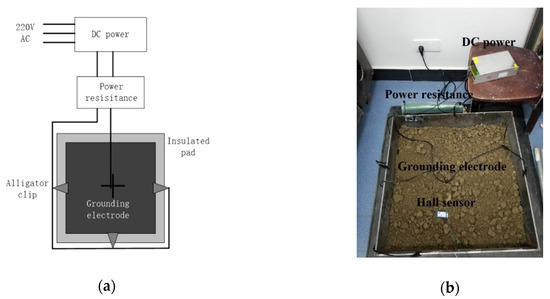
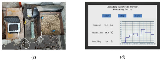
Figure 14.
The grounding electrode simulation environment platform. (a) The schematic of the grounding electrode simulation platform; (b) connection diagram of the measuring parts; (c) the entire environment of the experiment; (d) display interface of the current measuring device.
4.3. Analysis of Measurement Data
A total of 24 measuring points in the X and Y directions of the cross-shaped and ring-shaped grounding electrodes were selected. We measured the current 10 times at each measurement point and finally calculated their average value. The experimental data results are shown in Table 5, Table 6, Table 7 and Table 8, and the standard error is shown in Figure 15 and Figure 16. The standard error in the X and Y directions can be visually observed in space and projected onto the plane.
Table 5.
The current of measurement results and simulation results in the X and Y directions of the cross-shaped grounding electrode under the three-layer soil model.
Table 6.
The current of measurement results and simulation results in the X and Y directions of the ring-shaped grounding electrode under the three-layer soil model.
Table 7.
The current of measurement results and simulation results in the X and Y directions of the cross-shaped grounding electrode under the mixed-layer soil model.
Table 8.
The current of measurement results and simulation results in the X and Y directions of the ring-shaped grounding electrode under the mixed-layer soil model.
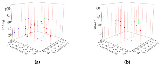
Figure 15.
The standard error of measurement under the three-layer soil model. (a) The standard error of the cross-shaped grounding electrode; (b) the standard error of the ring-shaped grounding electrode.
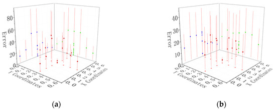
Figure 16.
The standard error of measurement under the mixed-layer soil model. (a) The standard error of the cross-shaped grounding electrode; (b) the standard error of the ring-shaped grounding electrode.
In the three-layer soil model, the standard error of the ring-shaped grounding electrode is significantly lower than 40% of the cross-shaped grounding electrode. In the mixed-layer soil model, the standard error of the ring-shaped grounding electrode is 50% lower than the cross-shaped grounding electrode. Therefore, under the same soil model, the measurement error of the ring-shaped grounding electrode is smaller than that of the cross-shaped grounding electrode, and it is confirmed that the ring-shaped grounding electrode has a better dispersion characteristic. Besides, the error between the current value measured by the current measuring device and the simulated value is always maintained at about 10%, which illustrates the reliability and usability of the device.
5. Conclusions
- (1)
- According to the special geological conditions of frozen soil and considering the difference in soil resistivity at different depths, this paper established a three-layer soil model and a mixed-layer soil model, using the finite element Galerkin method to study the dispersion characteristics of different grounding electrodes. The results show that the best to worst order of the dispersion characteristics of the three grounding electrodes is as follows: ring-shaped, cross-shaped, and linear. Furthermore, under the same conditions, the current and voltage in the soil around the ring-shaped grounding electrode are 35–40% lower than those of the linear grounding electrode.
- (2)
- Based on the simulation results, we built a grounding electrode simulation experiment platform in the laboratory. Then, we proposed a measurement scheme based on a “drainage wire” with a Hall sensor and designed and manufactured a grounding electrode current measurement device. The weak DC in soil around the grounding electrode can be measured in the laboratory, and the error can be compared with simulated data. It is found that the error is always maintained at about 10%, which confirms the feasibility of the scheme and the reliability of the measuring device.
Author Contributions
L.Z. performed the experiments and wrote the paper; H.J. contributed analysis tools; F.Y. conceived and designed the experiments; H.L. analyzed the data; W.L. and J.H. provided the experimental environment and the soil resistivity data of Inner Mongolia. All authors have read and agreed to the published version of the manuscript.
Funding
This research was funded by STATE GRID EAST INNER MONGOLIA ELECTRIC POWER MAINTENANCE COMPANY, grant number NO.SGTYHT/17-JS-199.
Conflicts of Interest
The authors declare no conflict of interest.
References
- Alassi, A.; Banales, S.; Ellabban, O.; Adam, G.; Maclver, C. HVDC Transmission: Technology Review, Market Trends and Future Outlook. Renew. Sustain. Energy Rev. 2019, 112, 530–554. [Google Scholar] [CrossRef]
- Bhuvaneswan, G.; Mahanta, B.C. Analysis of Converter Transformer Failure in HVDC Systems and Possible Solutions. IEEE Trans. Power Deliv. 2009, 24, 814–821. [Google Scholar] [CrossRef]
- Jiang, W.; Wu, G.N.; Wang, H.L. Calculation of DC grounding current distribution by UHVDC mono-polar operation with a ground return. In Proceedings of the Transmission & Distribution Conference & Exposition, Chicago, IL, USA, 21–24 April 2008. [Google Scholar]
- Sima, W.X.; Luo, D.H.; Yuan, T.; Liu, S.W.; Peng, Q.J.; Zhou, F.R. The influence of the vertical drop of the ground surface on the grounding resistance measurement of the grounding grid and the improvement measures. High Volt. Technol. 2018, 5, 1490–1498. (In Chinese) [Google Scholar]
- Liu, L.G.; Yu, Z.B.; Wang, Z.Z.; Li, M.; Wang, X.L. Analysis of the Monitoring Data of UHVDC Grounding Current Interference in a Buried Pipeline. IEEE Trans. Appl. Supercond. 2019. [Google Scholar] [CrossRef]
- Zhang, Y.; Dong, J.H.; Dong, X.G.; Wang, Y.S. Analysis of freezing and thawing of slope improved by soil nailing structure in seasonally frozen soil region. Rock Soil Mech. 2017, 38, 574–582. [Google Scholar]
- Zhang, B.; Zeng, R.; He, J.; Zhao, J.; Li, X.; Wang, Q.; Cui, X. Numerical analysis of potential distribution between ground electrodes of the HVDC system considering the effect of deep earth layers. IET Gener. Transm. Distrib. 2008, 2, 185–191. [Google Scholar] [CrossRef]
- Liu, L.G.; Ma, C.L. Calculation of ground potential distribution in multi-layer soil of DC transmission grounding electrode based on the finite element method. Power Syst. Protect. Control 2015, 18, 7–11. (In Chinese) [Google Scholar]
- Yang, W.Y.; Liu, J.; Wang, J.Y.; Shen, M.; Wang, X.F.; Li, Z.; Li, X.H. On-line monitoring of ground electrode of the HVDC transmission system. High Volt. Eng. 2006, 9, 15–17. (In Chinese) [Google Scholar]
- Zhang, Z.L.; Dan, Y.H.; Zou, J.; Liu, G.H.; Gao, C.F.; Li, Y.Q. Research on Discharging Current Distribution of Grounding Electrodes. IEEE Access 2019, 7, 59287–59298. [Google Scholar] [CrossRef]
- Teng, Y.; Wen, X.S.; Cai, H.S.; Jia, L.; Liu, G.; Hu, S.M.; Lu, H.L. Analysis on structural parameters and electrical performance of DC deep well-grounding electrode. J. Eng. 2019, 16, 2366–2370. [Google Scholar] [CrossRef]
- Zhou, L.J.; He, J.; Xu, H.; Wang, P.C.; Chen, Y.; Chen, S.X. Simulation of the impact of vertical grounding electrode on impulse grounding resistance of substation grounding network. In Proceedings of the IEEE International Conference on Integrated Circuits & Microsystems, Nanjing, China, 8–11 November 2017. [Google Scholar]
- Villas, J.E.T.; Portela, C.M. Calculation of electric field and potential distributions into soil and air media for a grounding electrode of an HVDC system. IEEE Trans. Power Deliv. 2003, 18, 867–873. [Google Scholar] [CrossRef]
- Xu, T.; Xu, Z.; Zhang, Z.R.; Zhou, Z.C.; Shen, Y. Calculation of current Field of circular grounding electrode for UHVDC transmission. High Volt. Eng. 2012, 6, 1445–1450. (In Chinese) [Google Scholar]
- Tomaskovicova, S.; Ingeman-Nielsen, T.; Christiansen, A.V.; Brandt, I.; Dahlin, T.; Elberling, B. Effect of electrode shape on grounding resistances—Part 2: Experimental results and cryospheric monitoring. Geophysics 2016, 81, WA169–WA182. [Google Scholar] [CrossRef]
- Zou, J.; Zeng, R.; He, J.L.; Guo, J.; Gao, Y.Q.; Chen, S.M. Numerical Green’s function of a point current source in horizontal multilayer soils by utilizing the vector matrix pencil technique. IEEE Transac. Magn. 2004, 40, 730–733. [Google Scholar] [CrossRef]
- Gouda, O.E.; El-Saied, T.; Salem, W.A.A.; Khater, A.M.A. Evaluations of the apparent soil resistivity and the reflection factor effects on the grounding grid performance in three-layer soils. IET Sci. Meas. Technol. 2019, 13, 572–581. [Google Scholar] [CrossRef]
- Dan, Y.H.; Zhang, Z.L.; Li, Y.Q.; Deng, J.; Zou, J. Novel Grounding Electrode Model with Axial Construction Space Consideration. Energies 2019, 12, 4765. [Google Scholar] [CrossRef]
- Zeng, R.; He, J.L.; Gao, Y.Q.; Zou, J.; Guan, Z.C. Grounding resistance measurement analysis of grounding system in vertical-layered soil. IEEE Trans. Power Deliv. 2004, 19, 1553–1559. [Google Scholar] [CrossRef]
- Choi, J.H.; Lee, B.H. An analysis on the Frequency-dependent grounding impedance based on the ground current dissipation of counterpoises in the two-layered soils. J. Electrost. 2012, 70, 184–191. [Google Scholar] [CrossRef]
- Tu, Y.P.; He, J.L.; Zeng, R. Lightning Impulse Performances of Grounding Devices Covered With Low-Resistivity Materials. IEEE Trans. Power Deliv. 2006, 21, 1706–1713. [Google Scholar] [CrossRef]
- Yutthagowith, P. Rogowski coil with a non-inverting integrator used for impulse current measurement in high-voltage tests. Electr. Power Syst. Res. 2016, 139, 101–108. [Google Scholar] [CrossRef]
- Yutthagowith, P.; Leelachariyakul, B. A Rogowski coil with an active integrator for measurement of long duration impulse currents. In Proceedings of the International Conference on Lightning Protection (ICLP), Shanghai, China, 11–18 October 2014. [Google Scholar]
- Ming, L.; Xin, Z.; Liu, W.; Loh, P.C. Structure and modeling of four-layer screen-returned PCB Rogowski coil with very few turns for high-bandwidth SiC current measurement. IET Power Electron. 2020, 13, 765–775. [Google Scholar] [CrossRef]
- Zhou, M.; Wang, J.G.; Cai, L.; Fan, Y.D.; Zheng, Z.N. Laboratory Investigations on Factors Affecting Soil Electrical Resistivity and the Measurement. IEEE Trans. Ind. Appl. 2015, 51, 5358–5365. [Google Scholar] [CrossRef]
- Seladji, S.; Cosenza, P.; Tabbagh, A.; Ranger, J.; Richard, G. The effect of compaction on soil electrical resistivity: A laboratory investigation. Eur. J. Soil Sci. 2010, 61, 1043–1055. [Google Scholar] [CrossRef]


Publisher’s Note: MDPI stays neutral with regard to jurisdictional claims in published maps and institutional affiliations. |
© 2020 by the authors. Licensee MDPI, Basel, Switzerland. This article is an open access article distributed under the terms and conditions of the Creative Commons Attribution (CC BY) license (http://creativecommons.org/licenses/by/4.0/).